Abstract
Handling missing values (MVs) and feature selection (FS) are vital preprocessing tasks for many pattern recognition, data mining, and machine learning (ML) applications, involving classification and regression problems. The existence of MVs in data badly affects making decisions. Hence, MVs have to be taken into consideration during preprocessing tasks as a critical problem. To this end, the authors proposed a new algorithm for manipulating MVs using FS. Bayesian ridge regression (BRR) is the most beneficial type of Bayesian regression. BRR estimates a probabilistic model of the regression problem. The proposed algorithm is dubbed as cumulative Bayesian ridge with similarity and Luca’s fuzzy entropy measure (CBRSL). CBRSL reveals how the fuzzy entropy FS used for selecting the candidate feature holding MVs aids in the prediction of the MVs within the selected feature using the Bayesian Ridge technique. CBRSL can be utilized to manipulate MVs within other features in a cumulative order; the filled features are incorporated within the BRR equation in order to predict the MVs for the next selected incomplete feature. An experimental analysis was conducted on four datasets holding MVs generated from three missingness mechanisms to compare CBRSL with state-of-the-art practical imputation methods. The performance was measured in terms of R2 score (determination coefficient), RMSE (root mean square error), and MAE (mean absolute error). Experimental results indicate that the accuracy and execution times differ depending on the amount of MVs, the dataset’s size, and the mechanism type of missingness. In addition, the results show that CBRSL can manipulate MVs generated from any missingness mechanism with a competitive accuracy against the compared methods.
1. Introduction
Data refers to cases or instances from the ambit that characterize the issue to be solved. In data management, one of the most important concerns is the quality of the data. Incomplete data often leads to bad decisions and negative analytics of the data. Researchers and analysts may face barriers when dealing with incomplete data. In addition, knowledge discovery becomes difficult to conduct with incomplete data, which means that the data quality comes first and foremost before working with the data [1]. The most popular form of data involves so-called tabular or structured data (i.e., rows of instances and columns of features for instances). The acquisition and collection of data may lead to errors in the data, for example, replicated entries, outliers, mixed formats, typos, MVs, etc. Error detection (i.e., errors are identified by experts) and error repair (i.e., bringing the data to a cleaner state) are the two phases of data cleaning. In research and industrial data, the presence of MVs causes loss of information [2]. Hence, the data preprocessing stage is needed to make the data clear and useful for analysis and knowledge extraction processes. Data preprocessing comprises two essential tasks: data preparation (e.g., handling MVs) and data reduction (e.g., feature selection). Most of the time and effort are dedicated to these tasks. To ensure accurate results, practitioners and theoreticians search for data preprocessing techniques.
The problems that are associated with MVs comprise bias; difficulties in analyzing the data; and loss of efficiency. Inadequate handling of MVs may result in deceitful findings derived from a research study. Several approaches have been elaborated to overcome the downsides produced by MVs; imputation is the most well-known approach. Imputation of MVs endeavors to fill in these MVs with predicted values. Relationships among the features can be defined because, in most cases, the features are not independent of each other [3].
Feature selection aims to remove redundant or irrelevant features (i.e., finding a minimum set of features). According to a specific criterion, FS chooses an optimal subset of features. The details of estimating feature subsets are determined by the selected criterion. The purposes of FS determine the selection of the criterion. In a nutshell, the main objective of FS is to identify the most important features in the dataset. The final dataset resulting from the sequence of data preprocessing can be considered suitable and useful for further work with the data [4].
1.1. Missing Data
This section introduces the missingness mechanism (i.e., the reason for the occurrence of MVs) and the traditional methods for handling MVs.
1.1.1. Missingness Mechanisms
Detecting the missingness mechanism is considered an important step for manipulating MVs. This paper considers and deals with the three kinds of missingness mechanisms [5,6,7,8].
For more illustrations of the different missingness mechanisms, consider that is a matrix whose elements are zeros or ones as indicators for missing and observed values, respectively, of the same size as the dataset that contains MVs. Indicate to the total dataset by , where represents the missing and represents the observed values. The distribution of is related to and to some unknown parameters . The probability for is described by . The three missing mechanisms are stated below.
MAR (Missing at random): the data are considered as MAR when does not depend on the MVs; the probability estimation is given by Equation (1):
MCAR (Missing completely at random): the data are considered as MCAR if the distribution of an instance having an MV for a feature does not depend on either complete or incomplete data (i.e., a special case of MAR); the probability estimation is given by Equation (2):
NMAR (Not missing at random): the data are considered as NMAR, also known as MNAR (missing not at random), when MV depends on both the value itself and the rest of the complete values; the probability estimation is given by Equation (3):
The next section introduces the most used approaches for handling MVs.
1.1.2. Simple Methods for Handling MVs
“Do not impute” is the simplest method, where all MVs are unsubstituted. Ignoring missing data (also known as case deletion) is another common method in the literature. Using the posterior method, all cases with one MV or more are deleted from the dataset. The only advantage of using case deletion comes when the data is MCAR; it leads to unbiased parameter estimates. In contrast, there is a lack of power when using case deletion. In addition, case deletion biases the results when the data is not MCAR. The results are biased when the data is MAR or MNAR. MVs are treated in one of three ways: (I) In complete case analysis (CCA), the instances that contain MVs on the features of interest are dropped from the data. (II) The other extreme is available case analysis (ACA), where, for each feature, all the responses in the data are used. The serious problem with these approaches is that MVs do not occur completely at random. (III) A more flexible method to deal with MVs is imputation.
Imputation approaches are most often used to handle nonresponse items. Imputation is defined as substituting an MV with a plausible value. There are many approaches for replacing an MV with a plausible value. The use of information in auxiliary or available data is a good method for improving data quality. The two approaches to impute MVs are single or multiple imputations.
Mean imputation replaces the MV of some feature with the sample mean computed from all observed values of that feature. Using mean imputation may distort correlations and relationships among features; it also distorts the distribution of the features. Regression imputation uses a regression model from complete cases to estimate MVs. Hot-deck imputation replaces MVs of the recipient variable (i.e., nonrespondent variable) with observed values from the donor variable (i.e., respondent variable). The random hot-deck method is a version of the hot-deck imputation approach in which there is a set of potential donors, and the random hot-deck approach selects the donor randomly. On the other hand, the deterministic hot-deck method selects specific donors based on some metrics. Cold-deck imputation uses auxiliary data as a source for MVs.
The imputed values resulting from the imputation methods mentioned above are treated as the ‘truth’, and the statistical methods use the completed dataset resulting from the imputation. Therefore, these imputation methods may cause underestimation of the variance, and all posterior analyses ignore that an imputation was conducted. Ignoring the uncertainty may lead to underestimating the variance. Multiple imputation [9] takes this uncertainty into consideration. The multiple imputation technique creates m imputations for each MV, and the analysis of the data uses these m completed datasets. Moreover, MVs can be predicted using ML techniques such as k-nearest neighbors (KNN), linear regression, or BRR.
The proposed algorithm depends on BRR given by Equation (4) [10] for predicting MVs.
where
The target variable is represented by which is distributed as a Gaussian distribution characterized by mean and variance . represents the independent features, and represents the unknown parameters. The number of independent features is denoted by . The regularization parameters are represented by and , which are assessed jointly during the fit of the model by maximizing the log marginal likelihood. Both of them are distributed as gamma distributions. are hyperparameters of the gamma prior distributions.
1.2. Feature Selection
Just as handling MVs is necessary for obtaining correct decisions, the machine learning-based classification techniques also play an important role in the decision-making process. In various applications, accuracy is considered very essential in classifiers. For example, but not limited to, a false negative with a high percentage in screening systems may increase the risk of the patients not receiving the required attention. Furthermore, a high false alarm rate increases the load on medical resources and causes undesired worries. For the purpose of obtaining a higher classification accuracy, feature selection (FS) has been applied for data reduction [11].
The problem of FS is defined as follows: for a set of given features, a subset is selected that fulfills the best under some classification system [12]. In other words, FS reduces the number of features. FS methods are intended to reduce the number of input features to those that are believed to be most useful to a model with the aim of predicting the target feature.
FS is expected to improve ML model performance, especially in circumstances defined by the high dimensionality data problem produced by quite a few training instances versus a large number of detected features. This type of circumstance occurs generally in medicine, where thoughtfulness of difficulty, cost, time, and risk problems may limit the number of training instances, while the number of disease markers increases quickly over the years [13].
Some predictive modeling problems may have a large number of features that require a large amount of memory and can slow the training and development of models. Additionally, the performance of models can degrade when comprising input features that are irrelevant to the target feature.
The two most important advantages of using FS are (1) reducing the cost of recognition and (2) providing a better classification accuracy [14]. FS is of high importance for two reasons: (I) prediction, i.e., improving the prediction performance of a target feature while dropping uninformative or irrelevant features, and (II) discovery, i.e., detecting features that actually depend on the target feature. In both cases, if features contain a large number of MVs, imputing these features may cause false positives. In the first situation, the prediction may not be harmed; however, in the second one, it will incorrectly choose unrelated features [11].
Similar to correlation, mutual information and fuzzy FS, the FS preprocessing step, are still of high importance despite the existence of MVs. Easy solution is to neglect features that hold large number of MVs (e.g., >50%). Nevertheless, dropping a feature may end in losing analytical power. In addition, losing the ability to recognize statistically considerable variations, and it usually generates bias, influencing badly the conclusions. FS needs to pay attention to the MVs’ mechanisms [3].
In this paper, we use the FS approach based on fuzzy entropy measures defined by De Luca and Termini [15] with the similarity-based classification procedure that was proposed in [16]. Fuzzy entropy is an FS method for choosing the most important features, and the measures of fuzzy entropy have been successfully used for the process of FS.
1.2.1. Similarity-Based Classification
Classification is an important technique in modern statistical approaches. It categorizes objects into distinct classes [17]. Many machine learning systems include classification, and pattern recognition is used in a variety of applications. In such systems, the accuracy of the classification is important since it supports decision making [18]. The classification phase assigns objects to definite classes (or categories) based on the information in the feature. The number of features that should be measured as well as the best of them are two critical factors to consider. Additionally, misclassification may cause heavy losses. Currently, classifiers are useful in online classifications that require decisions in a short time interval [19].
The idea behind measures of similarity is that there is a potential to find the similarity between two objects by comparing them, and a numerical value which is used during the classification is assigned to this similarity. Partitioning of the feature space in order to execute the classification is normally significant because it requires that the decisions be correct. Once partitioning is conducted conveniently, then classification can be conducted.
To provide greater elaboration about feature similarity classification, suppose we want to classify a set of objects into separate classes by their features. Luukka [16] assumed that is the number of features of diverse types that can be observed from the objects. We suppose that the values for the magnitude of each attribute are normalized so that they can be presented as a value between [0, 1]. Consequently, the objects we want to classify are vectors that belong to .
For every class, the ideal vector that denotes the class should be determined. By using some sample set of vectors which belong to a known class , can be calculated or user defined. The generalized mean given by Equation (5) can be used to calculate .
where is the power value obtained from the generalized mean. is fixed for all and values. The variable represents the number of samples in class .
After determining the ideal vectors, the decision for an arbitrary selected belonging to which class is made by a comparison between it and each ideal vector. The comparison can be accomplished through the use of similarity in the generalized Lukasiewicz structure [20] defined by Equation (6).
for . From the generalized Lukasiewicz structure, the parameter can be detected, and is a weight parameter. The weights were set as one. Luukka decided that if:
This means that the decision of whether the sample belongs to a specific class is made depending on the highest similarity value of the ideal vector.
1.2.2. Fuzzy Entropy & Similarity Classifier
A fuzzy set is a set of elements with different degrees of membership [21]. The elements in classical sets have full membership (i.e., the value of the membership is 1). On the other hand, a function is used to map the elements of the fuzzy set into a value belonging to a universe of interval values [0, 1] [22,23]. Based on the fuzzy set, fuzzy entropy is defined through the use of the membership function concept. De Luca and Termini [15] used Shannon’s function to define fuzzy entropy given by Equation (8).
where denotes the number of features, and the fuzzy values are represented by . represents the fuzzy set that performs the role of the maximum element of the ordering specified by when = 0.5.
Now, in the best circumstances, if the sample fits into the class , we acquire the similarity , and the similarity value equals zero if the sample does not fit into this class. The evaluation of fuzzy entropy is conducted using Equation (8). If we obtain high similarity values, we acquire low entropy values, and if the similarity values are close to 0.5, we acquire high entropy values. When the uncertainty is high, we obtain high entropy values, and we obtain low entropy values if similarities are high (or low). For manipulating MVs using an FS method, the mechanisms of the MVs must be taken into consideration [3].
The rest of the paper is organized as follows: Section 2 contains literature review about the analysis of MVs and FS. Section 3 presents the proposed algorithm. Section 4 illustrates the experimental setup. Section 5 discusses the results and discussion. The conclusion and future work are presented in Section 6.
1.3. Motivation and Contribution
Poor performance and the failure of many imputation algorithms during the manipulation of MVs encouraged the authors to propose an algorithm that handles these defects. The proposed approach manipulates the aforesaid deficiencies by utilization of the most operational features for dealing with MVs in a cumulative order.
The main contributions are that this paper provides a summary of the studies that deal with MVs and FS; proposes a new method for imputing missing values; overcomes the problems found in existing algorithms; and shows that the size of the dataset influences the performance metrics.
2. Literature Review
This section offers a short overview of the literature about MV manipulation and previous work that used FS to handle MVs.
2.1. The Problem of MVs
As previously emphasized, the problem of MVs is very well-known in ML and has therefore been extensively studied and analyzed in the literature for several purposes. Manipulating MVs essentially involves deletion, imputation, and learning instantly with MVs [24].
A deletion may be case deletion, also known as complete case analysis, which deletes instances that hold any MVs and only uses the complete ones for the analysis [6]. Obviously, case deletion may result in instances being lost, especially when the number of MVs is high and the MVs exist within several instances [25]. Deleting the feature which holds MVs more than a predefined percentage is known as “specific deletion”. In pair-wise deletion or variable deletion, where the instances that include MVs in the features within the current analysis are excluded, these features are used for other studies that do not involve the features that hold the MVs [2,3,24].
On the other hand, imputation benefits from the observed instances within the dataset to assess the missed values for producing complete datasets, and hence, imputation overcomes the disadvantages of the deletion method. Imputation can be classified into two classes: single imputation and multiple imputation. In single imputation, the missing value is imputed using a specific value [26]. In multiple imputation, the MVs are imputed m times, generating m complete datasets, and the final manipulated dataset is the average analysis of these m completely generated datasets [27]. The disadvantage of using multiple imputation is the need for more resources [28]. It is better than other methods such as deletion, maximum likelihood techniques, and single imputation [29]. The imputed value can be the mode, median, mean, or any predetermined value from the feature that has MVs [30], or it may be the result of a substitution case. Furthermore, imputed values can be assessed using cold-deck imputation [26], hot-deck imputation [31], expectation-maximization imputation [32,33], etc. Prediction models are also used to predict MVs after a model is built using the available information in the dataset [34]. Imputation methods are thought to be useful for manipulating MVs in situations such as when (I) the feature that holds MVs has a statistical impact on the output feature, (II) the MVs are of type MAR or MCAR, and (III) an instance does not hold MVs due to various features [35]. MVs of type MCAR may be manipulated using listwise deletion or maximum likelihood methods. On the other hand, there are no general approaches for dealing with MVs of the MNAR type [6,36].
One of the most extensively used imputation methods is KNN imputation, which consists of determining among the complete instances the k-nearest neighbors of the missing value. The MVs are then substituted with the average of these neighbors’ values. The performance of this method is limited, especially when the number of MVs is high [25]. FINNIM is a practical nonparametric iterative multiple imputation method that uses KNN to impute MVs [37]. Inverse probability weighting (IPW) methods are used to manipulate MVs depending on the weighting cases by describing the whole dataset, even the MVs using the inverse of the detected probability [3]. Some other multiple imputation methods are singular-value decomposition (SVD), ordinary least squares (OLS), and partial least squares (PLS), which are good methods for multiple imputation [6]. The manipulation of MVs in datasets that contain binary and ordinal features using the fully conditional specification (FCS) and multivariate normal imputation (MVNI) methods exhibits less biased and similar results [38].
The author of [5] proposed an imputation method based on similarities between the cases in the donor and the incomplete feature to impute the missing values. In [2], the author proposed a linear regression-based imputation technique. Each variable that is filled in is included in the equation periodically. In the same manner, the authors of [3] proposed an imputation technique for imputing missing values depending on the cumulative order with the aid of gain ratio (GR) feature selection. Likewise, the authors of [24] proposed two imputation algorithms for imputing missing values based on the Bayesian ridge technique. Their proposed algorithms work under two different feature selection conditions.
2.2. FS with MVs
Commonly, three approaches are used to achieve FS: wrappers, filters, and embedded methods. Wrappers are based on the performance prediction of a particular model and thus need many such models to be optimized, which can be very time-consuming in practice. Nevertheless, they are assumed to result in high-performance predictions, specifically because they are meant to maximize the model’s performance [25,39]. Filtering methods, on the other hand, look for a subset of features independent of any prediction algorithm, optimizing a criterion. The most common criteria used for FS are mutual information (MI), the correlation coefficient, or other information-theoretic quantities. Filters are generally used in practice as a result of their speed and simplicity [25]. Eventually, embedded methods that perform predictions and FS have earned a lot of consideration lately, particularly the original LASSO extensions [40].
Despite the importance of studying both MVs and FS concurrently, we have awareness of only the following studies: In [41], the authors attempted to estimate the MI distribution utilizing the Dirichlet second-order distribution to perform FS. The improvements were, however, restricted to the classification problem. In [42], the authors proposed to join FS and the imputation of MVs. Nevertheless, the FS was only used to increase the performance of a KNN, and it was not obvious if such a strategy can improve the algorithm performance. In [3,24], three novel algorithms were proposed to impute MVs depending on a specific FS condition such as correlation, gain ratio, and the feature with a lower number of MVs. In [2], a cumulative linear regression algorithm was proposed using linear regression as a predictive model to handle MVs. It operates well with both small and large datasets.
3. Proposed Algorithm
This section introduces the proposed algorithm in detail. The following procedural steps aid in explaining the proposed algorithm presented in Figure 1. The main objective of the steps of the proposed algorithm is to use the most informative feature to impute missing values with the appropriate values.
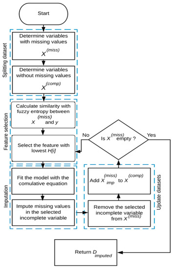
Figure 1.
Proposed algorithm flow chart.
Step 1: The proposed algorithm receives a dataset D as the input, which contains MVs, and then it separates D into two sets. The first set X(comp) incorporates all the complete features, and the second set X(mis) incorporates all the incomplete features. The output feature was assumed to be complete, so X(comp) includes all the perfect features and the target feature y. The importance of this step is obtaining two datasets, the in/complete datasets. The incomplete one will be used in the next steps.
Step 2: The proposed algorithm (CBRSL) uses the FS of the fuzzy entropy measure introduced by De Luca and Termini, given by Equation (8), with the similarity-based classification presented in Equation (6). The proposed algorithm looks for the feature that has a strong relationship with the target feature (i.e., selects the feature that offers the lowest fuzzy entropy). The importance of this step is the use of the most influencing feature among all features.
Step 3: After selecting the candidate variable , the model is fitted using the cumulative formula presented in Equation (9) with the candidate feature as dependent and as the independent feature. The selected feature is removed from , and after filling MVs within the , the filled feature is added to . Now, includes all the complete features, and . A new from is chosen. and are the new variables for the cumulative formula. The model is fitted with the cumulative formula, with as an independent feature and the new as the dependent feature.
where
where , is the number of features containing MVs, and is the number of complete independents. This step is the most important because it includes the formula that will be used in the imputation.
Step 4: Repeat Step 2 of feature selection until becomes empty. At that moment, return the imputed dataset () as described in Algorithm 1.
| Algorithm 1: CBRSL |
| 1: Input: 2: D: a dataset with MVs containing n instances. 3: Output: 4: Dimputed: a dataset with all missing features imputed. 5: Definitions: 6: Set of complete features. 7: Set of incomplete features. 8: . 9: Number of features containing MVs. 10: Fuzzy entropy measure with the similarity. 11: Begin 12: . 13: that exhibits #. 14: 15: . 16: 17: with the fitted model. 18: and add to . 19: End While 20: 21: End |
4. Experimental Setup
4.1. Datasets
Datasets were collected from many database repositories where they are available and freely accessible. To clarify that the proposed method is valid for different datasets, different datasets were used in cases and features. The fundamental specifications of the datasets used are shown in Table 1. In every dataset, the amounts, 10%, 20%, 30%, 40%, and 50%, of MVs were created for each missingness mechanism, MAR, MCAR, and MNAR, using the ampute function from the R environment [43]. As mentioned in Section 3, the output feature of each dataset was assumed to be complete, and all other features contained missing values. The proposed algorithm applies the cumulative equation for each incomplete dataset generated.

Table 1.
The fundamental specifications of the used datasets.
Breast Cancer Wisconsin Dataset: This dataset was designed by Dr. Wolberg, and the intention was to precisely diagnose breast masses depending solely on fine-needle aspiration (FNA). The resulting dataset is well known as the Wisconsin Breast Cancer Dataset.
Dermatology Dataset: This database includes 34 features, one of them is nominal and 33 of them are linear valued. The differential diagnosis of erythemato-squamous diseases is an extreme problem in dermatology. They all participate in the clinical features of scaling and erythema with very small variations. The diseases in this group are seborrheic dermatitis, psoriasis, lichen planus, chronic dermatitis, pityriasis rosea, and pityriasis rubra pilaris. Usually, a biopsy is essential for the examination, but unluckily, these diseases participate in various histopathological features as well. A different problem for the differential diagnosis is that a disease can display the features of different diseases in the starting stage and can hold the unique features in later stages. Patients were first assessed clinically with 12 features. Later, skin samples were selected for the calculation of 22 histopathological variables. The values of the histopathological variables are defined by sample analyses under a microscope.
Parkinson’s Dataset: This dataset was designed at the University of Oxford by Max Little. This dataset comprises a series of biomedical voice estimations from people with Parkinson’s disease (PD) and healthy people. The foremost purpose of the data is to classify healthy people from those with PD according to the “status” feature, which is set to zero for healthy and 1 for PD.
Pima Indians Diabetes Dataset: This dataset contains information on the presence or absence of diabetes among Pima Indian women living near Phoenix, Arizona. There are eight features: plasma glucose concentration; number of pregnancies; diastolic blood pressure (mmHg); serum insulin (µU/mL); tricep skin fold thickness (mm); diabetes pedigree function; body mass index (kg m−2); and age in years.
4.2. Performance Evaluation
A comparison was made between the proposed algorithm and five algorithms for the previous four datasets. The experiments were carried out using Python (version 3.7) and R (version 3.5.2). The compared algorithms are briefly described in Table 2. The performance evaluation was calculated for the five missingness ratios in terms of MAE, RMSE, and the R2 score.
Table 2.
The algorithms used in the comparison.
4.3. MAE and RMSE
Generally, MAE and RMSE were used as statistical metrics to measure the performance of the models [51]. MAE and RMSE are exhibited in Equations (10) and (11), respectively.
where and are the real and predicted values, respectively, of the case, and represents the number of the cases.
4.4. R2 Score
The R2 score, given by Equation (12), is a statistical measure that denotes how well the predicted values and real values are close to each other.
where
5. Analysis and Discussion
Figure 2, Figure 3, Figure 4 and Figure 5 exhibit the averages of the evaluation metrics for the five missingness ratios. The results show that the performance varies due to the missingness mechanisms, MV proportions, and size of the dataset. This section is divided into two subsections: the first subsection exhibits error analysis, and the second subsection offers accuracy analysis. A log scale is used in MAE and RMSE comparisons because each of them has a different range of values. Considering RMSE and MAE, a lower value is better so they can be collected in the same figure. On the other hand, an R2 score with a higher value is better. The computational complexity of the proposed algorithm is O (n).
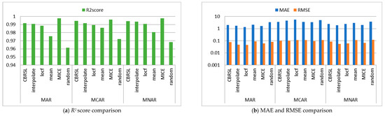
Figure 2.
Comparison between the proposed algorithm, interpolate, locf, mean, MICE and random methods (Parkinson’s Dataset).
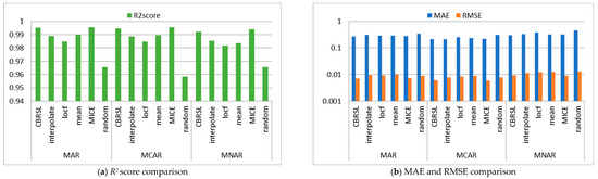
Figure 3.
Comparison between the proposed algorithm, interpolate, locf, mean, MICE and random methods (Dermatology Dataset).
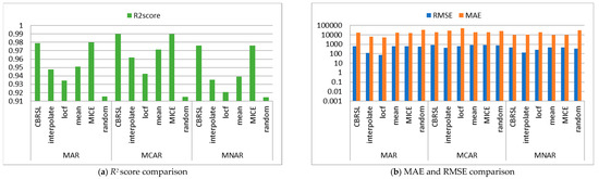
Figure 4.
Comparison between the proposed algorithm, interpolate, locf, mean, MICE and random methods (Breast Cancer Wisconsin Dataset).
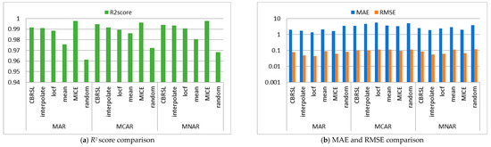
Figure 5.
Comparison between the proposed algorithm, interpolate, locf, mean, MICE and random methods (Pima Indians Diabetes Dataset).
5.1. Error Analysis
This subsection demonstrates that, in most cases, CBRSL offers lower errors. In what follows, the error analysis is presented in detail. The error analysis was interpreted by evaluating RMSE and MAE. It can be concluded that the error is small because all the features were used in the prediction of missing values.
From Figure 2b, for MAR, it was remarked that the MAE and RMSE of CBRSL are better than the mean and random methods and are worse than the interpolate, last observation carried forward (locf), and multivariate imputation by chained equations (MICE) methods. For MCAR, the MAE and RMSE of CBRSL are better than the interpolate, locf, mean, and random methods and are worse than MICE. For MNAR, the MAE and RMSE of CBRSL are better than the mean and random methods and are worse than the interpolate, locf, and MICE methods. From Figure 3b, it was observed that the RMSE and MAE are better than all the compared methods for MAR. For MCAR and MNAR, the MAE of CBRSL is better than all the compared methods, and the RMSE of CBRSL is better than all the compared methods but is worse than MICE. From Figure 4b, for MAR, it was observed that the MAE of CBRSL is better than the mean and random methods and is worse than the interpolate, locf, and MICE methods. In addition, the RMSE of CBRSL is better than the mean and MICE methods and is worse than the interpolate, locf, and random methods. CBRSL’s MAE equals the mean of the provided error for MCAR and outperforms the interpolate, locf, MICE, and random methods. In addition, the RMSE of CBRSL is better than the mean and MICE methods and is worse than the interpolate, locf, and random methods. CBRSL’s MAE equals the mean of the provided error for MCAR and outperforms the interpolate, locf, MICE, and random methods. In addition, the RMSE of CBRSL is better than the mean and MICE methods and is worse than the interpolate, locf, and random methods. From Figure 5b, for MAR and MNAR, it was observed that the MAE and RMSE of CBRSL are better than the mean and random methods and are worse than the interpolate, locf, and MICE methods. For MCAR, the MAE and RMSE of CBRSL are better than the interpolate, locf, mean, and random methods and are worse than MICE.
5.2. Accuracy Analysis
This subsection shows that in most cases, CBRSL offers better accuracy. In what follows, the accuracy analysis is discussed in detail. The accuracy analysis was interpreted by evaluating the R2 score. The improvement in accuracy results from using the most important and influential variable under the conditions stated in Section 3.
From Figure 2a, Figure 3a and Figure 5a, it was shown that the R2 score of CBRSL is better than the interpolate, locf, mean, and random methods and is worse than MICE for all missingness mechanisms. From Figure 4a for MAR, it was observed that the R2 score of CBRSL is better than the interpolate, locf, mean, and random methods and is worse than MICE. For MCAR, the R2 score of CBRSL is better than the interpolate, locf, mean, and random methods and is equal to MICE. For MNAR, the R2 score of CBRSL is better than the other stated methods.
The proposed algorithm depends on the BRR technique, which assumes that the target feature is distributed as a normal distribution, so CBRSL offers good a imputation accuracy when the target feature is Gaussian or Gaussian-like. Furthermore, it is considered a good choice to use transformers such as Box–Cox and Yeo–Johnson data before applying the proposed algorithm. In addition, the proposed algorithm includes a ridge parameter in which the ordinary least square is tuned to minimize the squared absolute sum, termed as L2 regularization. This method is effective in the case of collinearity between independent features, and training data will be overfitted by the ordinary least square.
6. Conclusions
MVs occur in nearly every analysis, and thus have become a universal problem. It is not recommended to use the delete method for cases that contain missing values. Facilitating the use of deletion may lead to data loss that may lead to undesirable results and expectations. Some of the algorithms currently in use result in insufficient accuracies. To this end, this paper proposes an imputation algorithm named CBRSL that manipulates MVs using FS. CBRSL is based on the notion of feature similarity measures and fuzzy entropy measures for performing the FS step, which has been proven to be efficient in classification problems, and the BRR technique for building the predictive model. The proposed algorithm handles MVs in a cumulative order, and the imputed features are incorporated with the other complete features to predict the MVs within the next candidate feature until all MVs in the dataset are imputed.
Hence, CBRSL benefits from the complete features to predict the incomplete features, hence utilizing the predicted features in the imputation of the incomplete features and so on. The proposed algorithm is simple to perform and does not fail in the imputation despite the volume of the dataset. In addition, the proposed algorithm succeeded in dealing with different percentages of MVs resulting from any missingness mechanism. The proposed algorithm is promising when handling MVs with new datasets. Additional units for selecting the candidate feature of the standard error will be used (such as the T-value and P-value). Furthermore, the proposed algorithm is considered to be beneficial in imputing inadequate medical datasets, such as cardiovascular disease data, DNA microarray data, food composition data, pulmonary embolism data, and other medical data. In the future, the proposed method will take into consideration some other techniques, such as classification and clustering.
Author Contributions
Conceptualization, A.S. and S.M.M.; methodology, A.S. and S.M.M.; software, A.S. and S.M.M.; validation, A.S., S.H. and S.M.M.; formal analysis, A.S., S.H. and S.M.M.; investigation, A.S., H.E., F.K.K. and S.M.M.; resources, A.S., H.E., F.K.K. and S.M.M.; data curation, A.S., S.H. and S.M.M.; writing—original draft preparation, A.S., H.E., F.K.K. and S.M.M.; writing—review and editing, A.S., H.E., F.K.K., S.H. and S.M.M.; visualization, A.S., H.E., F.K.K. and S.M.M.; supervision, H.E., F.K.K. and S.M.M.; project administration, H.E. and F.K.K.; funding acquisition, H.E. and F.K.K. All authors have read and agreed to the published version of the manuscript.
Funding
Princess Nourah bint Abdulrahman University Researchers Supporting Project number (PNURSP2022R300), Princess Nourah bint Abdulrahman University, Riyadh, Saudi Arabia.
Data Availability Statement
The data presented in this study are available on request.
Acknowledgments
This research project was funded by Princess Nourah bint Abdulrahman University Researchers Supporting Project number (PNURSP2022R300), Princess Nourah bint Abdulrahman University, Riyadh, Saudi Arabia.
Conflicts of Interest
The authors declare that they have no conflicts of interest to report regarding the present study.
References
- García, S.; Ramírez-Gallego, S.; Luengo, J.; Benítez, J.M.; Herrera, F. Big data preprocessing: Methods and prospects. Big Data Anal. 2016, 1, 1–22. [Google Scholar] [CrossRef]
- Mostafa, S.M. Imputing missing values using cumulative linear regression. CAAI Trans. Intell. Technol. 2019, 4, 182–200. [Google Scholar] [CrossRef]
- Mostafa, S.M.; Eladimy, A.S.; Hamad, S.; Amano, H. CBRG: A novel algorithm for handling missing data using bayesian ridge regression and feature selection based on gain ratio. IEEE Access 2020, 8, 216969–216985. [Google Scholar] [CrossRef]
- Chandrashekar, G.; Sahin, F. A survey on feature selection methods. Comput. Electr. Eng. 2014, 40, 16–28. [Google Scholar] [CrossRef]
- Mostafa, S.M. Missing data imputation by the aid of features similarities. Int. J. Big Data Manag. 2020, 1, 81–103. [Google Scholar] [CrossRef]
- Yadav, M.L.; Roychoudhury, B. Handling missing values: A study of popular imputation packages in R. Knowl.-Based Syst. 2018, 160, 104–118. [Google Scholar] [CrossRef]
- Chen, M.; Zhu, H.; Chen, Y.; Wang, Y. A Novel Missing Data Imputation Approach for Time Series Air Quality Data Based on Logistic Regression. Atmosphere 2022, 13, 1044. [Google Scholar] [CrossRef]
- Zhang, Y.; Thorburn, P.J. Handling missing data in near real-time environmental monitoring: A system and a review of selected methods. Future Gener. Comput. Syst. 2022, 128, 63–72. [Google Scholar] [CrossRef]
- Rubin, D.B. Multiple Imputation for Nonresponse in Surveys; Wiley: Hoboken, NJ, USA, 1987. [Google Scholar]
- Pedregosa, F.; Varoquaux, G.; Gramfort, A.; Michel, V.; Thirion, B.; Grisel, O.; Blondel, M.; Prettenhofer, P.; Weiss, R.; Dubourg, V.; et al. Scikit-learn: Machine learning in Python. J. Mach. Learn. Res. 2011, 12, 2825–2830. [Google Scholar]
- Seijo-Pardo, B.; Alonso-Betanzos, A.; Bennett, K.P.; Bolón-Canedo, V.; Josse, J.; Saeed, M.; Guyon, I. Biases in feature selection with missing data. Neurocomputing 2019, 342, 97–112. [Google Scholar] [CrossRef]
- Jain, A.; Zongker, D. Feature selection: Evaluation, application, and small sample performance. IEEE Trans. Pattern Anal. Mach. Intell. 1997, 19, 153–158. [Google Scholar] [CrossRef]
- Lewin, D.I. Getting clinical about neural networks. IEEE Intell. Syst. Appl. 2000, 15, 2–5. [Google Scholar] [CrossRef][Green Version]
- Jain, A.K.; Chandrasekaran, B. 39 Dimensionality and sample size considerations in pattern recognition practice. Handb. Stat. 1982, 2, 835–855. [Google Scholar]
- de Luca, A.; Termini, S. A definition of a nonprobabilistic entropy in the setting of fuzzy sets theory. Inf. Control 1972, 20, 301–312. [Google Scholar] [CrossRef]
- Luukka, P. Feature selection using fuzzy entropy measures with similarity classifier. Expert Syst. Appl. 2011, 38, 4600–4607. [Google Scholar] [CrossRef]
- Dougherty, G. Feature extraction and selection. In Pattern Recognition and Classification: An Introduction; Springer: New York, NY, USA, 2013; pp. 157–176. [Google Scholar]
- Venables, W.N.; Ripley, B.D. Classification. In Modern Applied Statistics with S-PLUS, Statistics and Computing; Springer: New York, NY, USA, 2002; pp. 331–351. [Google Scholar]
- Kurama, O. Similarity Based Classification Methods with Different Aggregation Operators. Ph.D. Thesis, Lappeenranta University of Technology, Lappeenranta, Finland, 2017. [Google Scholar]
- Luukka, P.; Saastamoinen, K.; Kononen, V. A classifier based on the maximal fuzzy similarity in the generalized Lukasiewicz-structure. In Proceedings of the 10th IEEE International Conference on Fuzzy Systems. (Cat. No.01CH37297), Melbourne, VIC, Australia, 2–5 December 2001; pp. 195–198. [Google Scholar]
- Zadeh, L.A. Fuzzy Sets and Information Granularity. Advances in Fuzzy Set Theory and Applications. 1979, pp. 3–18. Available online: https://www2.eecs.berkeley.edu/Pubs/TechRpts/1979/ERL-m-79-45.pdf (accessed on 15 August 2022).
- Revanasiddappa, M.B.; Harish, B.S. A New feature selection method based on intuitionistic fuzzy entropy to categorize text documents. Int. J. Interact. Multimed. Artif. Intell. 2018, 5, 106–117. [Google Scholar] [CrossRef]
- Zadeh, L.A. Fuzzy sets. Inf. Control 1965, 8, 338–353. [Google Scholar] [CrossRef]
- Mostafa, S.M.; Eladimy, A.S.; Hamad, S.; Amano, H. CBRL and CBRC: Novel algorithms for improving missing value imputation accuracy based on bayesian ridge regression. Symmetry 2020, 12, 1594. [Google Scholar] [CrossRef]
- Doquire, G.; Verleysen, M. Feature selection with missing data using mutual information estimators. Neurocomputing 2012, 90, 3–11. [Google Scholar] [CrossRef]
- Farhangfar, A.; Kurgan, L.A.; Pedrycz, W. A Novel framework for imputation of missing values in databases. IEEE Trans. Syst. Man Cybern. Part A Syst. Hum. 2007, 37, 692–709. [Google Scholar] [CrossRef]
- Horton, N.J.; Lipsitz, S.R. Multiple imputation in practice: Comparison of software packages for regression models with missing variables. Am. Stat. 2001, 55, 244–254. [Google Scholar] [CrossRef]
- Fichman, M.; Cummings, J.N. Multiple imputation for missing data: Making the most of what you know. Organ. Res. Methods 2003, 6, 282–308. [Google Scholar] [CrossRef]
- Graham, J.W. Missing data analysis: Making it work in the real world. Annu. Rev. Psychol. 2009, 60, 549–576. [Google Scholar] [CrossRef] [PubMed]
- Bertsimas, D.; Pawlowski, C.; Zhuo, Y.D. From predictive methods to missing data imputation: An optimization approach. J. Mach. Learn. Res. 2018, 18, 1–39. [Google Scholar]
- Ma, Z.; Chen, G. Bayesian methods for dealing with missing data problems. J. Korean Stat. Soc. 2018, 47, 297–313. [Google Scholar] [CrossRef]
- Razavi-Far, R.; Cheng, B.; Saif, M.; Ahmadi, M. Similarity-learning information-fusion schemes for missing data imputation. Knowledge-Based Systems 2020, 187, 104805. [Google Scholar] [CrossRef]
- Do, C.B.; Batzoglou, S. What is the expectation maximization algorithm? Nat. Biotechnol. 2008, 26, 897–899. [Google Scholar] [CrossRef]
- Jiang, H. Defect features recognition in 3D Industrial CT Images. Informatica 2018, 42, 477–482. [Google Scholar] [CrossRef]
- Royston, P. Multiple imputation of missing values. Stata J. 2004, 4, 227–241. [Google Scholar] [CrossRef]
- Acock, A.C. Working with missing values. J. Marriage Fam. 2004, 67, 1012–1028. [Google Scholar] [CrossRef]
- Sahri, Z.; Yusof, R.; Watada, J. FINNIM: Iterative imputation of missing values in dissolved gas analysis dataset. IEEE Trans. Ind. Inform. 2014, 10, 2093–2102. [Google Scholar] [CrossRef]
- Lee, K.J.; Carlin, J.B. Multiple imputation for missing data: Fully conditional specification versus multivariate normal imputation. Am. J. Epidemiol. 2010, 171, 624–632. [Google Scholar] [CrossRef]
- Khalid, S.; Khalil, T.; Nasreen, S. A survey of feature selection and feature extraction techniques in machine learning. In Proceedings of the 2014 Science and Information Conference, London, UK, 27–29 August 2014; pp. 372–378. [Google Scholar]
- Zou, H.; Hastie, T. Regularization and variable selection via the elastic net. J. R. Stat. Soc. 2005, 67, 301–320. [Google Scholar] [CrossRef]
- Zaffalon, M.; Hutter, M. Robust feature selection by mutual information distributions. In Proceedings of the Eighteenth Conference on Uncertainty in Artificial Intelligence (UAI2002), Edmonton, AB, Canada, 1–4 August 2002; pp. 577–584. [Google Scholar]
- Meesad, P.; Hengpraprohm, K. Combination of knn-based feature selection and knn based missing-value imputation of microarray data. In Proceedings of the International Conference on Innovative Computing, Information and Control, Dalian, China, 18–20 June 2008; p. 341. [Google Scholar]
- Van Buuren, S. MICE: Multivariate Imputation by Chained Equations. 2021. Available online: https://cran.r-project.org/web/packages/mice/index.html (accessed on 1 August 2022).
- Wi, H. Wolberg, Breast Cancer Wisconsin. 1992. Available online: https://archive.ics.uci.edu/ml/datasets/breast+cancer+wisconsin+(original) (accessed on 1 August 2022).
- Ilter, M.D.N.; Guvenir, H.A. Dermatology. 1998. Available online: https://archive.ics.uci.edu/ml/datasets/dermatology (accessed on 4 August 2022).
- Max Little, Parkinsons. 2008. Available online: https://archive.ics.uci.edu/ml/datasets/parkinsons (accessed on 4 August 2022).
- Rossi, R.A.; Nesreen, K. Ahmed, Pima Indians Diabetes. 1990. Available online: http://networkrepository.com/pima-indians-diabetes.php (accessed on 2 August 2022).
- Donders, A.R.T.; van der Heijden, G.J.M.G.; Stijnen, T.; Moons, K.G.M. Review: A gentle introduction to imputation of missing values. J. Clin. Epidemiol. 2006, 59, 1087–1091. [Google Scholar] [CrossRef] [PubMed]
- Kearney, J.; Barkat, S. Autoimpute. 2019. Available online: https://autoimpute.readthedocs.io/en/latest/ (accessed on 2 August 2022).
- Law, E. Impyute. 2017. Available online: https://impyute.readthedocs.io/en/master/ (accessed on 1 August 2022).
- Chai, T.; Draxler, R.R. Root mean square error (RMSE) or mean absolute error (MAE)?—Arguments against avoiding RMSE in the literature. Geosci. Model Dev. 2014, 7, 1247–1250. [Google Scholar] [CrossRef]
Publisher’s Note: MDPI stays neutral with regard to jurisdictional claims in published maps and institutional affiliations. |
© 2022 by the authors. Licensee MDPI, Basel, Switzerland. This article is an open access article distributed under the terms and conditions of the Creative Commons Attribution (CC BY) license (https://creativecommons.org/licenses/by/4.0/).