Research on Power Price Forecasting Based on PSO-XGBoost

Abstract

With the reform of the power system, the prediction of power market pricing has become one of the key problems that needs to be solved in time. Power price prediction plays an important role in maximizing the profits of the participants in the power market and making full use of power energy. In order to improve the prediction accuracy of the power price, this paper proposes a power price prediction method based on PSO optimization of the XGBoost model, which optimizes eight main parameters of the XGBoost model through particle swarm optimization to improve the prediction accuracy of the XGBoost model. Using the electricity price data of Australia from January to December 2019, the proposed model is compared with the XGBoost model. The experimental results show that PSO can effectively improve the performance of the model. In addition, the prediction results of PSO-XGBoost are compared with those of SVM, LSTM, ARIMA, RW and XGBoost, and the average relative error and root mean square error of different power price prediction models are calculated. The experimental results show that the prediction accuracy of the PSO-XGBoost model is higher and more in line with the actual trend of power price change.

1. Introduction

Power is an important basic industry and public utility related to the national economy and people’s livelihoods. The main purpose of a power market reform is to break the monopoly, improve the production efficiency of the power industry and realize the optimal allocation of resources by introducing the competition mechanism. Chile [1] was the first country to marketize the electricity market. In 1982, Chile officially promulgated new electricity laws and regulations, which defined the position that the transmission system is open to all domestic power plants and all individual electricity users in the form of official national laws, thus changing the situation of a regional monopoly and starting a new reform in the operation of contract electricity trading and real-time electricity trading; therefore, various power enterprises’ operation changed from monopoly to competition. The power system in Chile has achieved the expected results, which not only ensures the basic stability of electricity prices, but also ensures that power producers can obtain considerable profits; however, some problems are also exposed, including the lack of investment in grid development caused by the imperfect pricing of electricity sales and the imperfect pricing system of the transmission system. After decades of development, the reform of the electricity market in the UK has achieved many phased results [2]. After four stages of electricity market reform, Britain has established a fair, transparent and open electricity trading market, and introduced privatization and competition through the four aspects of power generation, electricity sales, distribution and electricity sales. However, with the continuous practice of electricity reform, the British electricity market has also exposed some drawbacks, such as the complexity of system marginal price calculations, and the quotations of power producers can not truly reflect their power generation costs. Since the 1990s, China has successively carried out the practice and exploration of electricity marketization reform [3,4,5,6], and provinces (regions) have carried out various types of reform practices, including transmission and distribution price verification, electricity sales side reform, direct trading, etc., in combination with policy requirements and their own actual conditions. However, it was not until August 27, 2019, when the State Grid Corporation of China issued the Notice of the Ministry of Industry of the State Grid on the Withdrawal of Electricity Sales by Collective Enterprises of the Company System, requiring the collective enterprises of the company system to withdraw from the electricity sales business, that China’s electricity sales side was fully opened, forming a market structure of multiple buyers and sellers, breaking the monopoly of the power grid on the power industry, and making great progress in the construction of electricity marketization. However, there are still problems, such as untimely information disclosure, inadequate market supervision and imperfect pricing mechanisms. The National Energy Market (NEM) of Australia is one of the well-known free-bidding electricity markets in the world. Its electricity reform was based on the experiences and lessons of other countries and adjustments were made according to local conditions. The reform of electricity marketization in Australia has roughly gone through three stages: the structural restructuring of the electricity industry, building a unified electricity market system and re-establishing the electricity regulatory system [7]; it has always focused on providing users with lower electricity prices, promoting competition among internal departments of the power industry, optimizing energy investment and providing open access to the power network [8]. After decades of development, Australia’s power system reform has achieved remarkable results, not only in reducing electricity prices and improving the efficiency of the power industry, but also in increasing investment in the power industry, which improved the competitiveness of Australia’s industry. To sum up, the electric power system reform in various countries aims to achieve the following objectives: 1. provide a stable electricity price and power supply; 2. break monopoly barriers and improve competitiveness; and 3. improve the transparency and satisfaction of power trading, and make the power market truly fair, just and open.

With the continuous advancement of the reforms of the power system and the liberalization of the power sales side in various countries, the power trading market has gradually become the leading development trend in the current power industry, and power resources have become a commodity. The power price is the core content of power market transactions, and power price forecasting is of great significance for the fair trading and supply–demand interaction of all players in the power market. For power producers, they need to make bidding strategies based on an accurate forecast of power prices to meet the principle of maximum income and minimum risk, and accurate forecasting of power prices can enable power producers to accurately grasp the market trends and then formulate the best price strategy. For power purchasers, the accurate prediction of power prices can enable power purchasers to effectively control power consumption and reasonably plan for power consumption according to their own actual conditions, thus reducing the cost of electricity consumption. For market regulation, the accurate prediction of electricity price can provide a scientific basis for formulating various electricity policies, promote the development and progress of the electricity market, and promote the formation of a stable, orderly and healthy market environment [9]. Therefore, power price forecasting is of great significance. Combined with the historical data on power pricing, this paper uses the PSO-optimized XGBoost to forecast the power price, establishes a power price forecasting model based on the PSO-optimized XGBoost, and compares this model with other models to prove the effectiveness and correctness of PSO-XGBoost.

2. Related Work

The importance of power price forecasting has attracted the attention and research of many scholars at home and abroad. At present, the prediction methods of power price mainly include the grey model prediction method, neural network method and combination model prediction method.

In 1982, Professor Deng of Huazhong University of Science and Technology first pro-posed the grey system theory [10]. At present, many scholars have studied the grey model in power price forecasting [11]. The main research object of grey system theory is the uncertain system of “poor information”. It realizes an accurate description and under-standing of the real world through part of the known information and finds internal laws. After 40 years of development, grey system theory has been widely used in many fields, such as society, water conservancy, medicine and so on, and has achieved good results [11]. Reference [10] improves the traditional grey model and uses the improved grey model to forecast the clearing price of the power market. In order to improve the prediction accuracy, the authors of [12] established an improved grey model of multi-electricity prices to comprehensively predict the electricity price in the spot market and the long-term contract market, and adopted the grey solution optimization algorithm.

Reference [13] uses autoregressive integrated moving average (ARIMA) models to predict the next day’s electricity price, and corrects the error of the prediction model. In order to improve the convergence speed, the authors of [14] designed a Levenberg–Marquardt BP (LMBP) method to train the neural network, which is used to predict the short-term electricity price, and carried out experiments in the electricity market of Anhui Province, proving the high performance of this method. Article [15] combines an artificial neural network and clustering algorithm, proposes a day-ahead price prediction model based on an RNN and tests it on the hourly price of daytime electricity in the US electricity market. In order to improve the accuracy and stability of power price forecasting, the authors of [16] proposed an optimized long short-term memory neural network (LSTM) model and tested it in the power markets of Pennsylvania, New Jersey and Maryland. Reference [17] proposed a deep RNN-based day-ahead price forecasting method, and verified it based on the data of the New England power market, where the results showed that the method was effective. Reference [9] proposes a price forecasting method based on genetic algorithm, which uses genetic algorithm to optimize BP neural network, and tests it on the data of the American power market. The experimental results show that this method can effectively control the forecasting error. In order to improve the accuracy of electricity price prediction, article [18] adopts the method of a deep belief network to predict the day-ahead electricity price, and uses the real data of the PJM power market in the United States to simulate the prediction. The experimental results show that the prediction accuracy of the deep belief network is higher, and it is an effective method for power prediction.

In view of the low prediction accuracy of a single model in power price prediction [19], many scholars have proposed combined prediction methods. Reference [20] proposes a hybrid model of EMD-LSTM-SVR to predict the power price. EMD is used to extract the periodic component and the trend component in the power price sequence, and LSTM is used to predict the periodic component and the trend component and output the prediction results of each component. Support vector regression (SVR) is used to superimpose the prediction sequence of each component to generate the predicted price sequence. Finally, the precision of the model is predicted using the price data of the PJM power market in the United States. In order to improve the prediction accuracy by taking advantage of the unique characteristics of each model, the authors of [21] proposed a hybrid method that combines a wavelet transform with a kernel extreme learning machine based on the adaptive particle swarm optimization and autoregressive moving average (ARMA), and evaluates the performance of this method by using the electricity price data of five countries. Reference [22] combines the ensemble empirical mode decomposition (EEMD), support vector machine (SVM) and autoregressive moving average (ARMA) to form a combined prediction model, and uses the real data of American power sales companies for prediction. The experimental results show that the combined model has a higher prediction accuracy. On the basis of the conventional electricity price forecasting model, article [23] also established an ARIMA forecasting model for the random sequence formed by the predicted residual to correct the electricity price forecasting results. The combined model can improve the prediction accuracy to a certain extent, but it also has many shortcomings, such as not being able to depict the linear change trend in the power price series.

To sum up, in order to improve the accuracy of power price prediction and characterize the changing trend of power pricing, this paper optimizes the extreme gradient boosting (XGBoost) based on particle swarm optimization (PSO), proposes a PSO-XGBoost power price prediction method and tests it on the Australian power price dataset from January to December 2019.

3. PSO-XGBoost

This section introduces the XGBoost algorithm and PSO algorithm, explains how PSO optimizes the main parameters of XGBoost, and proposes two evaluation indicators of the model.

3.1. XGBoost

XGBoost was proposed by Chen [24] in 2016 and is an improved Gradient Boosting Decision Tree(GBDT). Boosting is an algorithm that promotes the combination of base classifiers with strong classifiers. First, a base classifier is trained using the initial training set, and the weight of the training samples in the next base classifier is adjusted according to the performance so that the samples with classification errors gain more attention; this is repeated many times until they meet the conditions. Finally, the trained multiple classifiers are weighted and combined. Compared with GBDT, XGBoost is characterized by a high accuracy, difficulty in overfitting, and strong scalability [25].The objective function of GBDT is the loss function, and the objective function of XGBoost is the loss function plus the regular term. The loss function is the difference between the predicted value and the real value, and the objective function is optimized by reducing the loss; the regular term is used to control the complexity of the model and prevent extreme cases of the model.

Assuming that there are K trees in the model [26,27], for the sample set $\left\{\left(x_1,y_1\right),\left(x_2,y_2\right),\cdots ,\left(x_m,y_m\right)\right\}$, the prediction value of the model for each sample value $x_i$ is:

$${\widehat{y}}_i={{\displaystyle \sum }}_{k=1}^K{f}_k\left(x_i\right)={\widehat{y}}_i^{t-1}+f_t\left(x_i\right),$$

(1)

where $f_t\left(x_i\right)=\mathrm{q}\left(x_i\right)$ represents the leaf node corresponding to the sample on the kth weak classifier.

The objective function of XGBoost is the loss function plus the regular term. The over-all objective function can be expressed as:

$$\mathrm{L}={{\displaystyle \sum }}_{i=1}l\left(y_i,y_i^{*}\right)+{{\displaystyle \sum }}_k\mathsf{\Omega }\left(f_k\right),$$

(2)

where ${\displaystyle \sum }_{i=1}l\left(y_i,y_i^{*}\right)$ represents the loss function composed of the deviation between the real value and the predicted value, and ${\displaystyle \sum }_k\mathsf{\Omega }\left(f_k\right)$ represents the regular term, which is used to prevent the model from overfitting. It is expressed as follows:

$$\mathsf{\Omega }\left(f\right)=\gamma T+\frac{1}{2}\lambda {{\displaystyle \sum }}_{j=1}^T{w}_j{}^2,$$

(3)

where T is the number of leaf nodes, $\gamma$ and $\lambda$ are parameters that control the structure of the tree and the weight distribution of leaf nodes, and $w_j$ is the weight of leaf nodes with index j.

According to Formulas (1) and (2), the overall objective function is converted into the following form:

$$\mathrm{L}\left(k\right)={{\displaystyle \sum }}_{i=1}l\left(y_i,{\widehat{y}}_i^{t-1}+f_t\left(x_i\right)\right)+{{\displaystyle \sum }}_k\mathsf{\Omega }\left(f_k\right)$$

(4)

Expand the loss function by using the second-order Taylor expansion and remove the constant term to obtain a new objective function as follows:

$$w_j^{*}=\frac{G_j}{H_j+\lambda },$$

(5)

where $g_i=\frac{\partial l\left(y_i,{\widehat{y}}_i^{k-1}\right)}{\partial {\widehat{y}}_i^{k-1}}$ and $h_i=\frac{{\partial }^{2}l\left(y_i.{\widehat{y}}_i^{k-1}\right)}{\partial {\widehat{y}}_i^{2\left(k-1\right)}}$ are the second derivative of the loss function.

The optimal weight of the leaf node is:

$$\mathrm{L}\left(k\right)={{\displaystyle \sum }}_{i=1}^n\left(g_i{f}_t\left(x_i\right)+\frac{1}{2}{h}_i{f}_t^2\left(x_i\right)\right)+\mathsf{\Omega }\left(f_k\right),$$

(6)

where $G_j={\displaystyle \sum }_{i\in I_J}{g}_i$ is the sum of the accumulated values of the first-order partial derivatives contained in the leaf node j, and $H_j={\displaystyle \sum }_{i\in I_j}{h}_i$ is the sum of the second-order partial derivatives contained in the leaf node j.

The objective function is rewritten as a quadratic function of one variable with respect to the leaf weight w and the optimal value of the objective function is:

$$\mathrm{L}\left(k\right)=-\frac{1}{2}{{\displaystyle \sum }}_{j=1}^T\frac{G_j^2}{H_j+\lambda }+\gamma T$$

(7)

3.2. Particle Swarm Optimization

Particle swarm optimization (PSO) was proposed by Kennedy and Eberhart in 1995 [28]. Its basic idea is to simulate the predatory behavior of birds that adjust their search path and then find food according to their own experience and population communication. Each solution in the solution space of PSO corresponds to a bird in the search space, which is called a particle. Each particle has two characteristics of position and velocity. Each position of the particle represents a feasible solution. The particle moves in the space at a certain speed. The particle’s running track is the process of solving. In the iterative process of particle swarm, the search process of each particle is constrained by the individual extreme value and the group extreme value. The individual extreme value is the optimal position that the particle seeks itself, which is recorded as pBest. The group extreme value is the optimal position that the whole particle swarm currently finds, which is recorded as gBest. During the iteration, the velocity $v_i$ and position $x_i$ of the ith particle are calculated as follows [29]:

$$\begin{array}{c}{v}_i\left(t+1\right)=\omega \times v_i\left(t\right)+c_1\times rand\left(t\right)\times \left(pBes{t}_i-x_i\left(t\right)\right)+c_2\times rand\left(t\right)\times \\ \left(gBes{t}_i-x_i\left(t\right)\right),\end{array}$$

(8)

$$x_i\left(t+1\right)=x_i\left(t\right)+v_i\left(t+1\right),$$

(9)

where $\omega$ is the inertia factor, and its value is non-negative; $rand\left(t\right)$ is a random number between (0, 1); and c₁ and c₂ are learning factors, and usually, c₁ = c₂ = 2.

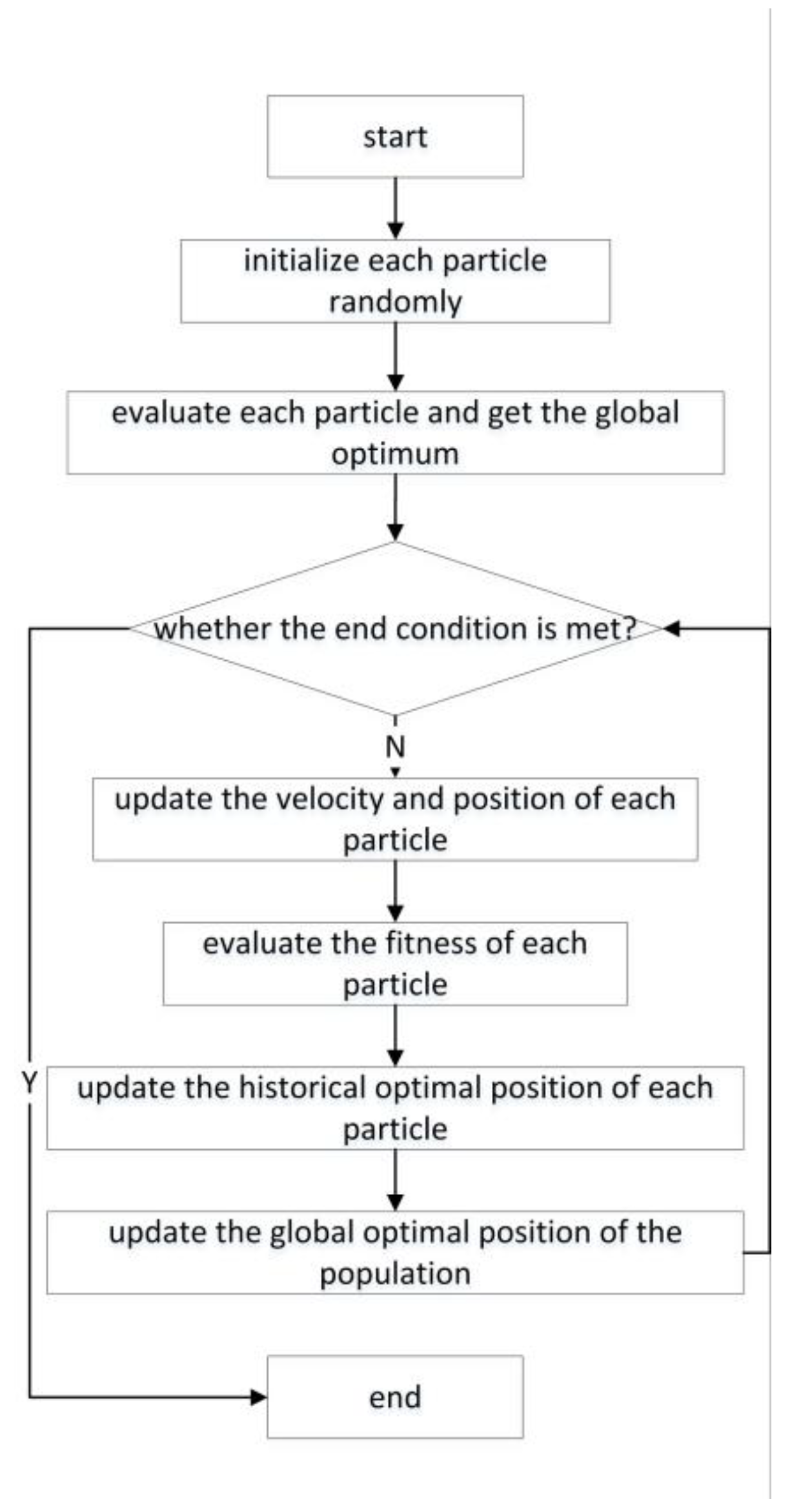
The flow chart of the PSO iterative search for the optimal solution is shown in Figure 1. The specific steps are as follows:

(1)

Randomly initialize the velocity and position of each particle in the search space.

(2)

Calculate the fitness value of each particle.

(3)

For each particle, its fitness value is compared with its best position pBest. If the current fitness value is better, it is taken as the current best position.

(4)

For each particle, its fitness value is compared with the global best position gBest. If the current fitness value is better, it is taken as the current best position.

(5)

Adjust the particle velocity according to Formula (8).

(6)

Adjust the position of the particles according to Formula (9).

(7)

Judge whether the end conditions are met. If the conditions are met, end the iteration. Otherwise, go to step (2) to continue the iteration.

3.3. PSO-XGBoost

There are many parameters in the XGBoost model. The main factor affecting the accuracy of the model is the setting of parameters. It is often impossible to find an accurate parameter by artificially setting parameters. Therefore, in this experiment, PSO is used to optimize the main parameters of XGBoost. The default values and value ranges of parameters are shown in

Table 1. Main parameters of XGBoost model.

Parameters	Default Value	Value Range
learning_rate	0.3	[0, 1]
max_depth	6	[0, +∞]
colsample_bytree	1	(0, 1]
subsample	1	(0, 1]
min_child_weight	1	[0, +∞]
gamma	0	[0, +∞]
reg_alpha	0	[0, +∞]
reg_lambda	1	[0, +∞]

.

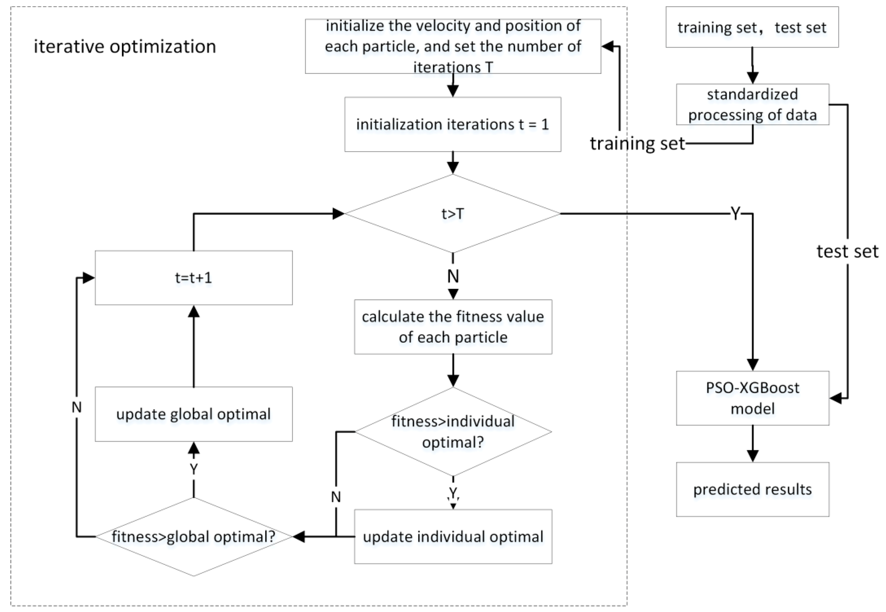
The flow chart of the PSO-XGBoost model is shown in Figure 2. The steps to build the PSO-XGBoost model are as follows:

(1)

The data set is divided into a training set and a test set. The training set is the power price data from 1 January 2019 to 30 January 2019, and the test set is the data from 31 January 2019. The training set is used for model training and parameter optimization, and the test set is used for checking the accuracy of the model.

(2)

The Z-score was used to standardize the training set and the test set.

(3)

Set the maximum number of iterations to 600, and set the inertia factor $\mathsf{\omega }$ the decrease as the number of iterations increases, with a decreasing range of 0.9 → 0.4.

(4)

Initialize the velocity and position of each particle according to the value range of the parameters.

(5)

The calculation formula of the fitness value is as follows:

$$\mathrm{I}=\frac{1}{N}{{\displaystyle \sum }}_{i=1}^N\left|y_i-y_i^{*}\right|,$$

(10)

where N is the total number of samples, $y_i$ is the actual value of the electricity price, and $y_i^{*}$ is the predicted value of the electricity price.

(6)

Start the iterative calculation, update the velocity and position of each particle according to Formulas (8) and (9), and calculate the updated fitness value according to Formula (10).

(7)

Adaptation value comparison. First, it is judged whether the fitness value is greater than the individual optimum. If the fitness value is greater than the individual optimum, the individual optimum is updated; otherwise, the individual optimum remains unchanged. Secondly, it is judged whether the fitness value is greater than the global optimum. If the fitness value is greater than the global optimum, the global optimum is updated; otherwise, the global optimum remains unchanged.

(8)

Update iterations: $t=t+1$.

(9)

Determine whether to terminate the iteration according to the iteration termination condition (satisfying the objective function or the maximum number of iterations). If the iteration terminates, go to the next step; otherwise, return to step (6) to continue the iteration.

(10)

The test set is used to predict the electricity price and output the prediction results.

The experimental results show that when the learning_rate is 0.01, max_depth is 3, colsample_bytree is 0.6, subsample is 0.7, min_child_weight is 1, gamma is 0.1, reg_alpha is 0.1 and reg_lambda is 0.1, the prediction effect of the PSO-XGBoost model is the best.

3.4. Evaluation Criteria of the Model

In this paper, the mean relative error (MRE) and root mean square error (RMSE) are used as the overall measurement standards of prediction accuracy to evaluate the performance of models after training. MRE is the average value of the relative error, which is a basic index to investigate the error; RMSE is the square root of the ratio of the square of the deviation between the predicted value and the real value of the model and the number of prediction times n. It is very sensitive to the large or small errors in the prediction data and can better reflect the accuracy of the prediction results [30]. The specific calculation formulas are as follows [31]:

$$E_{MRE}=\frac{1}{N}{{\displaystyle \sum }}_{i=1}^N\frac{\left|y_i-y_i^{*}\right|}{y_i}\times 100\%,$$

(11)

$$E_{RMSE}=\sqrt{\frac{1}{N}{{\displaystyle \sum }}_{i=1}^N{\left(y_i-y_i^{*}\right)}^2},$$

(12)

where N represents the total number of samples in the test set, $y_i$ represents the actual electricity price, and $y_i^{*}$ represents the predicted value.

4. Results

First, this section introduces the datasets used in the experiment and explains how to preprocess the datasets. Secondly, the PSO-XGBoost algorithm proposed in this paper is compared with other algorithm models. The comparison is mainly divided into two parts. Part one is the comparison between the PSO-XGBoost and XGBoost algorithm. The comparison results show that PSO can effectively optimize the parameters of XGBoost, thus improving the prediction accuracy. The second part is the comparison between PSO-XGBoost and other models. The experimental results show that PSO-XGBoost is more in line with the trend of power price changes and has higher accuracy.

4.1. Data Set

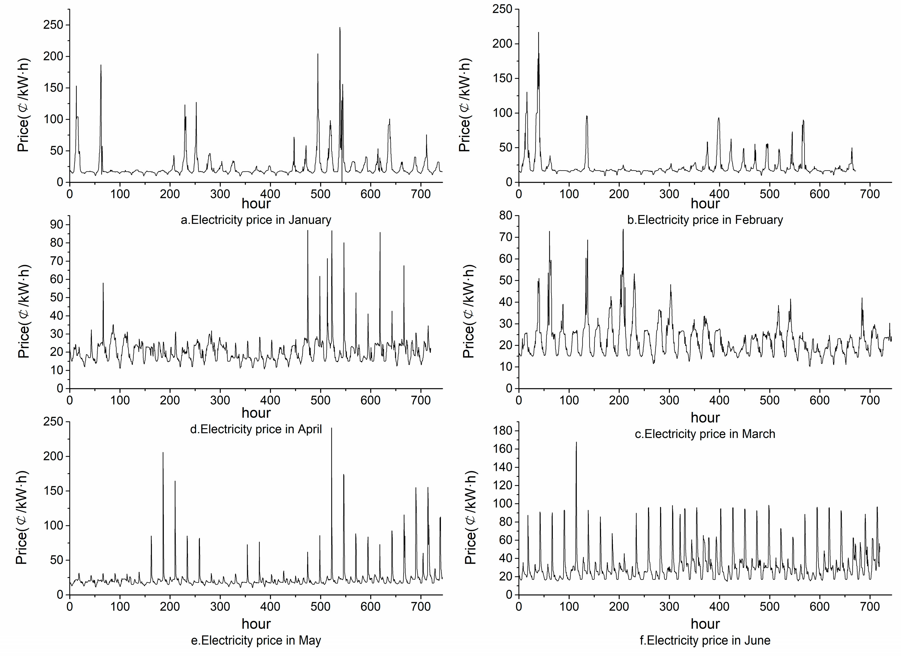
This paper uses the hourly power price data published by the Australian power market from January 2019 to June 2019 as the original data sequence for training and testing. The last day of each month is used as the test set, and the remaining data are used as the experimental training set. Six algorithms, XGBoost, LSTM, ARIMA [32], RW [33], SVR and PSO-XGBoost, are used to establish the power price prediction model. The change in the electricity price data from January 2019 to June 2019 is shown in Figure 3.

4.2. Feature of Data Set

In order to ensure that the model has sufficient feature information for training, the data set is divided into two parts: time characteristics and price data characteristics.

The prediction of the electricity price belongs to the time series problem, which often has periodicity, and the time information greatly affects the accuracy of the model. The electricity price has obvious periodicity, as, for example, there is a certain periodicity between the electricity price of the hour h on day d and the electricity price of the hour h on day d-1, as shown in

Table 2. Time features.

Feature Name	Feature Description
Day of the week	Day of the week
Hour of the day	Which hour of the day

. In this paper, two time characteristics related to power price forecasting are extracted.

When processing power price data, two aspects are mainly considered: one is the power price at adjacent time points, and the other is the power price at the same time point on adjacent days. The electricity price at adjacent time points mainly considers the influence of the electricity price adjacent to the forecast day d on the electricity price of the forecast day; the electricity price at the same time point on adjacent days mainly considers the periodicity of data by day. Specific features are shown in

Table 3. Features of price data.

Feature Name	Feature Description
Electricity price at time d-1	Electricity price at adjacent time points
Electricity price at time d-24	Electricity price at the same time point on adjacent days

.

4.3. Data Preprocessing

The Z-score normalization method is used to process the data to make it conform to the standard normal distribution. The formula is as follows:

$$x^{\prime }=\frac{x-mean\left(x\right)}{\sigma \left(x\right)},$$

(13)

where $x^{\prime }$ represents the value after standardization,$x$ represents the original value, $mean\left(x\right)$ represents the average value of the data, and $\sigma \left(x\right)$ represents the standard deviation of the data.

4.4. Analysis of Experimental Results

4.4.1. Experimental Results

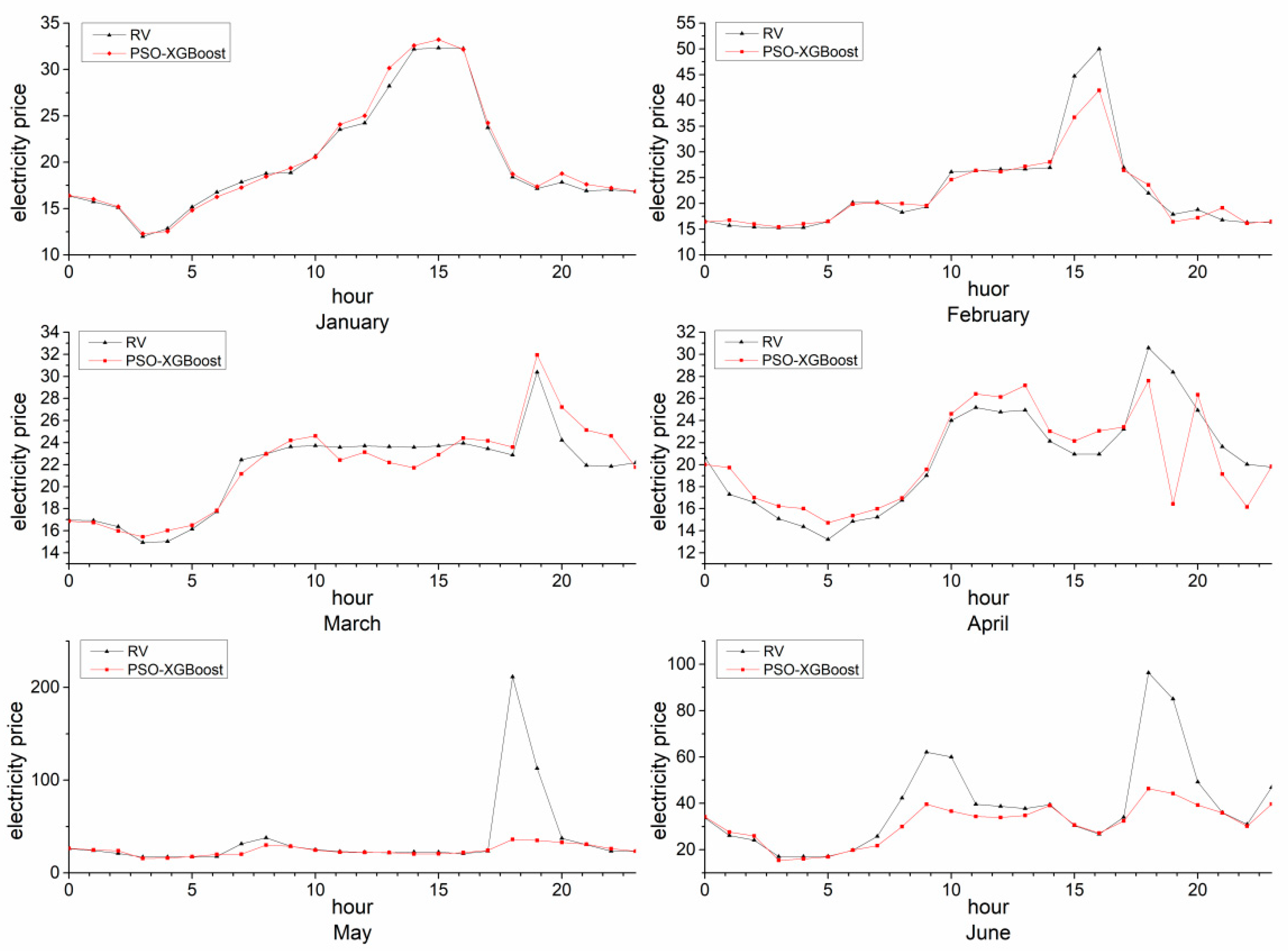
After the training of the power price prediction model based on PSO-XGBoost is completed, the model is used to predict the power price change from January to June 2019. The prediction results are shown in Figure 4, where RV represents the change curve of the actual value of the power price, and PV represents the change curve of the power price predicted by PSO-XGBoost. It can be seen from Figure 4 that the predicted value of the power price is close to the actual value, and the predicted change curve of the power price is basically consistent with the actual change trend, which indicates that the prediction effect is good.

4.4.2. Compared with XGBoost

In order to intuitively observe the parameter optimization effect of PSO on the XGBoost model, Figure 5 shows the prediction comparison between the XGBoost prediction model and the PSO-XGBoost prediction model from January to June. In the training process of the XGBoost model, we use 5-fold cross-validation to optimize the super parameters of XGBoost, evaluate the models corresponding to each group of parameters, and finally, select the best model and parameters. For 5-fold cross-validation, the data set is randomly divided into five parts, four of which are used as training data and one as test data for testing in turn. The corresponding deviation value will be obtained for each test, and the average value of the five results will be used as the evaluation index of the algorithm accuracy. The parameters of the XGBoost model are set as: the learning_rate is 0.01, max_depth is 6, colsample_bytree is 1, subsample is 0.7, min_ child_ weight is 1, gamma is 0.03, reg_alpha is 0.1 and reg_ lambda is 0.1. It can be seen from Figure 5 that both models have good effects, but the performance of PSO-XGBoost is better than XGBoost, and the predicted power price is closer to the actual price, which shows the effectiveness of PSO in improving the performance of the model. At the same time, compared with XGBoost, PSO-XGBoost can select parameters more intelligently, requires less manual experience, and has better theoretical value and practical significance.

4.4.3. Compared with Other Models

In order to compare the prediction effect of the PSO-XGBoost model proposed in this paper, extreme gradient boosting (XGBoost), the autoregressive integrated moving average model (ARIMA), random walks (RW), long short-term memory (LSTM) and support vector regression (SVR) are used to establish power price prediction models. The parameters of LSTM are set as follows: the LSTM layer is made up of three layers, where the number of neurons in the first layer is 64, the number of neurons in the second layer is 32, the number of neurons in the third layer is 16, the number of neurons in the fully connected layer is 1, the number of epochs is 100, and the batch size is 5. The parameters of SVR are set as follows: the kernel function is the Gaussian radial basis function, the penalty coefficient is 1e3, and gamma is 0.1. For ARIMA, the data set is basically stabilized after the first difference. Set the parameters of d = 1, p = 4, and q = 2 of the ARIMA model, and select the ARIMA (4,1,2) model. For RW, we chose a one-dimensional random walks model for comparison.

In order to more intuitively understand the prediction error at each time, Figure 6 shows the change trend of the actual power price and the predicted power price, where RV represents the actual value of the power price from January to June 2019. It can be seen from Figure 6 that the predicted value of the PSO-XGBoost model is closer to the actual power price at each time, and the power price change curve is more closely fitted to the actual power price change curve. PSO-XGBoost captures the original power price more regularly, and the prediction accuracy is higher than that of other comparison models.

According to the calculation formulas of the MRE and RMSE,

Table 4. MRE of different algorithms from January to June.

Month	MRE
	PSO-XGBoost	ARIMA	RW	XGBoost	LSTM	SVR
January	0.0224	0.0638	0.1440	0.1299	0.1782	0.2827
February	0.0499	0.0936	0.0967	0.1208	0.1883	0.1597
March	0.0451	0.0921	0.1103	0.1042	0.0942	0.0852
April	0.0811	0.0799	0.0874	0.1412	0.1544	0.1127
May	0.1307	0.1403	0.1269	0.1804	0.1562	0.1552
June	0.1837	0.1837	0.1687	0.1382	0.1546	0.1546

and

Table 5. RMSE of different algorithms from January to June.

Month	MRE
	PSO-XGBoost	ARIMA	RW	XGBoost	LSTM	SVR
January	0.6081	2.1963	2.9909	4.0098	3.8109	5.9029
February	2.5083	3.6091	3.7523	4.9329	5.8599	5.9019
March	1.3374	3.3073	3.2774	3.0893	2.5913	2.7165
April	2.9208	2.0741	2.3539	3.9655	4.7230	2.8429
May	39.2473	39.7893	39.5829	38.4477	40.6982	40.3427
June	15.3014	17.8628	17.7223	16.3771	16.5870	16.5059

show the MRE and RMSE of the prediction results of each model. It can be seen from the error comparison in Table 4 and Table 5 that the MRE and RMSE of the XGBoost improved based on PSO are smaller, and have better simulation and prediction effects.

4.5. Analysis of Experimental Results

In order to fully prove the effectiveness of the method proposed in this paper, in addition to fitting the electricity price data from January to June 2019, we also fitted the electricity price data from July to December and calculated the MRE and RMSE. There are 31 days (744 data) in July, August, October and December. We use the electricity price data of the first 24 days as the training set to train the model, and the data of the last 7 days as the prediction set to test the accuracy of the model. For the data of September and November, we use the data of the first 27 days as the training set, and the data of the last three days as the test set. The calculated MRE and RMSE are shown in

Table 6. MRE of different algorithms from July to December.

Month	MRE
	PSO-XGBoost	ARIMA	RW	XGBoost	LSTM	SVR
July	0.0932	0.0972	0.1014	0.1437	0.1723	0.1567
August	0.0874	0.0973	0.1253	0.1381	0.1923	0.1609
September	0.1047	0.0999	0.1123	0.1482	0.1375	0.1259
October	0.1063	0.1161	0.1082	0.1131	0.1459	0.1027
November	0.1471	0.1505	0.1628	0.1847	0.1629	0.1743
December	0.1207	0.1326	0.1640	0.1809	0.1298	0.1298

and

Table 7. RMSE of different algorithms from July to December.

Month	MRE
	PSO-XGBoost	ARIMA	RW	XGBoost	LSTM	SVR
July	6.9651	7.4569	7.6795	10.2248	11.6426	9.7482
August	2.3113	3.1528	2.4278	3.5036	3.4473	2.3393
September	1.2072	2.0222	2.0203	2.5119	4.2071	3.5206
October	24.2422	24.2922	25.6748	30.5328	32.1754	29.0631
November	1.5541	1.4704	1.6936	2.4317	3.4983	2.3604
December	29.2056	30.1172	30.0912	31.4767	35.6138	32.3558

.

5. Conclusions

This paper studies power price prediction in the power market. Taking the Australian power market as the background, a power price prediction model based on the PSO-improved XGBoost is established and verified using a data set from Australia from January to December 2019. The experimental results show that the XGBoost model optimized by PSO can obtain a prediction effect close to the actual value. In addition, this paper also sets up a comparative test. The LSTM price prediction model, XGBoost price prediction model and SVR price prediction model are established to compare results with the PSO-XGBoost model proposed in this paper, and the MRE and RMSE of the prediction results of different algorithms on the same data set are calculated. The data show that the MRE and RMSE of PSO-XGBoost are the smallest.

At present, the PSO-XGBoost proposed in this paper has some details that need to be improved, such as the balance between the number of iterations or particles and the optimal solution. When the number of particles or the number of iterations is set to be small, the algorithm runs for a short time, but it is easy to obtain the local optimal solution. On the contrary, if the algorithm runs for a long time, it can obtain the optimal solution. In the future, we need to continue to study and solve these problems and strive to improve the prediction accuracy of the model. I believe that our model will play an important role in the international power industry and China’s power system reform in the near future.

References

1. Shang, Y.Q.; Tian, G.D. Practice and status quo of foreign power market. Ind. Technol. Econ. 2002, 1, 72–73. [Google Scholar]
2. Zhang, X.P.; Li, J.N.; Fu, H. Reform and Challenge of UK Electricity Retail Market. Power Syst. Autom. 2016, 40, 10–16. [Google Scholar] [CrossRef]
3. Zhou, S.Y. Simulations of Bidding in Medium and Long-term Electricity Market based on Multi-agent Modeling. Master’s Thesis, Southeast University, Nanjing, China, 1 June 2019. [Google Scholar]
4. Chen, Y.P.; Qin, Z.J. Summary of research on electricity market reform. Electr. Electron. 2019, 4, 6–12. [Google Scholar]
5. The Communist Party of China (CPC) Central Committee and State Council of PRC. Opinions on Further Deepening the Reforms of Electricity Power System. Available online: http://www.cec.org.cn/huanbao/xingyexinxi/fazhangaige/2015-03-25/135625.html (accessed on 25 March 2015).
6. Song, Y.H.; Bao, M.L.; Ding, Y.; Shao, C.Z.; Shang, N. Summary of key points and relevant suggestions of China’s power spot market construction under the new power reform. Chin. Soc. Electr. Eng. 2020, 40, 10. [Google Scholar]
7. Huang, L.M.; Ma, L.; Zhang, X.X. Review of Australian Electricity Market in 2016. State Grid 2014, 6, 70–73. [Google Scholar]
8. Li, D.J.; Li, J.B.; He, Z.M. The Management and Operation of Australian Electricity Market and Its Enlightenment to China. Jilin Electr. Power 2004, 3, 6–9. [Google Scholar]
9. Bai, R.; Luo, G.; Tang, L.; Bai, S. Short term price forecasting of high proportion wind power based on genetic algorithm. Yangtze River 2022, 53, 119–124. [Google Scholar]
10. Cheng, C.; Luo, B.; Miao, S.; Wu, X. Mid-Term Electricity Market Clearing Price Forecasting with Sparse Data: A Case in Newly-Reformed Yunnan Electricity Market. Energies 2016, 9, 804. [Google Scholar] [CrossRef] [Green Version]
11. Wang, Z.D. Research on planning technology of large-scale hub erection base based on Grey System Theory. Technol. Ind. 2021, 21, 292–298. [Google Scholar]
12. Fan, Y.H.; Zhang, W.; Ding, X.; Xu, Q.S. Improved grey model for forecasting spot and medium and long-term market prices of electric power. Dig. Manag. Sci. 2018, 22, 45–49. [Google Scholar]
13. Contreras, J.; Espinola, R.; Nogales, F.J.; Conejo, A.J. ARIMA models to predict next-day electricity prices. IEEE Trans. Power Syst. 2002, 18, 1010–1020. [Google Scholar] [CrossRef]
14. Ranjbar, M.; Soleymani, S.; Sadati, N.; Ranjbar, A.M. Electricity Price Forecasting Using Artificial Neural Network. In Proceedings of the 2006 International Conference on Power Electronic, Drives and Energy Systems, New Delhi, India, 12–15 December 2006; pp. 1–5. [Google Scholar]
15. Panapakidis, I.P.; Dagoumas, A.S. Day-ahead electricity price forecasting via the application of artificial neural network based models. Appl. Energy 2016, 172, 132–151. [Google Scholar] [CrossRef]
16. Zhou, A.; Zhou, L.; Mao, M.; Tai, H.M.; Wam, Y. An Optimized Heterogeneous Structure LSTM Network for Electricity Price Forecasting. IEEE Access 2019, 7, 108161–108173. [Google Scholar] [CrossRef]
17. Zhang, C.; LI, R.; Shi, H. Deep learning for day-ahead electricity price forecasting. IET Smart Grid 2020, 3, 462–469. [Google Scholar] [CrossRef]
18. Guo, C.; Li, X.R.; Han, Z.Y.; Fu, X.Q. Day ahead price forecasting based on deep belief network. Power Demand Side Manag. 2022, 24, 86–91. [Google Scholar]
19. Qin, H.Y. Research on the application of combined model in power price forecasting. Comput. Simul. 2010, 27, 116–119. [Google Scholar]
20. Gou, X.; Xiao, X.Y. Short term electricity price forecasting model based on empirical mode decomposition and LSTM neural network. J. Xi’an Univ. Technol. 2020, 36, 129–134. [Google Scholar]
21. Zhang, Y.; Li, C.; Li, L. Electricity price forecasting by a hybrid model, combining wavelet transform, ARMA and kernel-based extreme learning machine methods. Appl. Energy 2017, 190, 291–305. [Google Scholar]
22. Zhang, J.L.; Wang, M.X. Electricity price forecasting based on EEMD, SVM and ARMA combined model. Power Demand Side Manag. 2020, 22, 63–68. [Google Scholar]
23. Zhou, M.; Yan, Z.; Ni, Y.X.; Li, G.Y. Arima power price forecasting method with error prediction correction. Chin. J. Electr. Eng. 2004, 12, 67–72. [Google Scholar]
24. Chen, T.Q.; Carlos, G. XGBoost: A Scalable Tree Boosting System. Assoc. Comput. Mach. 2016, 10, 785–794. [Google Scholar]
25. Zhang, C.; Chen, C.; Xu, H.Q. XGBoost: A Scalable Tree Boosting System. J. Agric. Mach. 2022, 53, 149–156. [Google Scholar]
26. Sun, C.; Lv, Q.; Zhu, S.T.; Zheng, W.; Cao, Y.F.; Wang, J. Ultra short term power load forecasting based on double-layer XGBoost algorithm considering multi feature effects. High Volt. Technol. 2021, 48, 2885–2898. [Google Scholar]
27. Li, N.; Zhang, J.H. Power System Transient Stability Assessment Method Based on XGboost-DF. Electr. Meas. Instrum. 2022, 13, 1–10. [Google Scholar]
28. Banks, A.; Vincent, J.; Anyakoha, C. A review of particle swarm optimization. Part I: Background and development. Nat. Comput. 2007, 64, 467–484. [Google Scholar] [CrossRef]
29. Wei, Y. Study on Non invasive Continuous Blood Pressure Measurement Based on PSO-GRNN Neural Network. Master’s Thesis, Jilin University, Changchun, China, 2022. [Google Scholar]
30. Tan, H.W.; Yang, Q.L.; Xing, J.C.; Huang, K.F.; Zhao, S.; Hu, H.Y. Photovoltaic power prediction based on xgboost LSTM combined model. J. Sol. Energy 2022, 43, 75–81. [Google Scholar]
31. Chen, Z.Y.; Liu, J.B.; Li, C.; Ji, X.H.; Li, D.P.; Huang, Y.H.; Di, F.C.; Gao, X.Y.; Xu, L.Z. Ultra short term power load forecasting based on LSTM and XGBoost combined model. Power Grid Technol. 2020, 22, 614–620. [Google Scholar]
32. Masini, R.P.; Medeiros, M.C.; Mendes, E.F. Machine learning advances for time series forecasting. J. Econ. Surv. 2021, 2012, 12802–12842. [Google Scholar] [CrossRef]
33. Medeiros, M.C.; Vasconcelos, G.F.; Veiga, Á.; Zilberman, E. Forecasting inflation in a data-rich environment: The benefits of machine learning methods. J. Bus. Econ. Stat. 2021, 39, 98–119. [Google Scholar] [CrossRef]
Figure 1. Flow chart of PSO.
Electronics 11 03763 g001
Figure 2. Flow chart of PSO-XGBoost.
Electronics 11 03763 g002
Figure 3. Data on electricity prices.
Electronics 11 03763 g003
Figure 4. Comparison between test set and prediction results.
Electronics 11 03763 g004
Figure 5. Comparison between XGBoost and PSO-XGBoost.
Electronics 11 03763 g005
Figure 6. Comparisons with other models.
Electronics 11 03763 g006