Article

Accelerated Chambolle Projection Algorithms for Image Restoration

School of Mathematics and Statistics, Xidian University, Xi’an 710071, China
*
Author to whom correspondence should be addressed.
These authors contributed equally to this work.
Electronics 2022, 11(22), 3751; https://doi.org/10.3390/electronics11223751
Submission received: 22 October 2022 / Revised: 10 November 2022 / Accepted: 11 November 2022 / Published: 15 November 2022
(This article belongs to the Section Computer Science & Engineering)

Abstract

:
In this paper, the accelerated Chambolle projection algorithms based on Frank–Wolfe have been proposed. For solving the image restoration under the additive Gaussian noise, the Chambolle projection method (CP) is widely used. However, the projection operator has a large computational cost and complex form. By means of the Frank–Wolfe method, this projection operation can be greatly simplified. We propose two new algorithms, called Chambolle projection based on Frank–Wolfe (CP–FW) and Chambolle projection based on accelerated Frank–Wolfe (CP–AFW). They have a fast convergence rate and low computation cost. Furthermore, we extend the new algorithms to deal with the Poisson noise. The convergence of the new algorithms is discussed, and results of the experiment show their effectiveness and efficiency.

1. Introduction

In image processing, minimizing the total variation energy functional is popular [1,2,3,4]. Recently, many variants of the total variation energy the functional model, the fractional total variation [5], the high-order total variation [6], directional total variation [7], and total generalized variation [8] have been applied for denoising, deblurring, inpainting, and other tasks. For solving the minimizing total variation, plenty of scholars have studied algorithms, for example, the standard [9] or non-standard discretization scheme [10], operator splitting [11,12,13], the Chambolle–Pock dual algorithm [11,14], the alternating direction method [15,16,17], and the Chambolle projection [4].
For solving the image restoration under the additive Gaussian noise, the Chambolle projection method (CP) is widely used. However, the projection operator has a large computational cost and complex form. By means of the Frank–Wolfe method, this projection operation can be greatly simplified.
In this paper, we propose new accelerated Chambolle projection algorithms for Gaussian denoising, according to the work of Chambolle. We call our new methods Chambolle projection based on Frank–Wolfe (CP–FW) and Chambolle projection based on accelerated Frank–Wolfe (CP–AFW). Meanwhile, we generalize the new algorithms under the Poisson noise condition. The convergence of algorithms is proved. Experiments show the better convergence rate of new algorithms and a low computational cost.
The outline of this paper is organized as follows. In Section 2, we show the related works and declare the notation. In Section 3, new algorithms are proposed under the Gaussian noise condition and a theoretical analysis is given. In Section 4, we extend these algorithms for Poisson noise removal. Section 5 shows the experiments of new algorithms. In Section 6, we summarize this paper.

2. Related Works

In this section, we first review the Chambolle projection algorithms for minimizing the total variation under the Gaussian noise. Then, the Frank–Wolfe method is briefly discussed.

2.1. Chambolle Projection Algorithm

For f = u + n , minimizing total variation [18] under the Gaussian noise has
min u E u = f u 2 2 2 λ + Ω u ,
where f is the observed image, u is the clean image, n is the additive white Gaussian noise (AWGN), Ω is the image domain, and λ is a regularization parameter to keep trade-off between data fidelity term and regularization term. | | · | | 2 denotes the L 2 norm (for convenience, we rewrite | | · | | 2 2 as | | · | | 2 in this paper). Ω u is a semi-norm in the bounded variation (BV) space.
For convenience, let J u = Ω u . Then, the Euler–Lagrange equation for (1) is shown as follows:
0 1 λ u f + J u ,
where is a sub-differential operator of J u . Define w J u ; then, (2) can be written as
f u λ J u u J * f u λ ,
where J * is the conjugate function of J. Then,
0 f u λ f λ + 1 λ J * f u λ .
We obtain w = f u λ is the minimizer of
min w w f λ 2 2 + J * w λ .
Since J * is the indicator function χ K w , where K is the closure of the set
d i v p | p C c 1 Ω , R 2 , p x 1 , x Ω ,
where C c 1 Ω , R 2 represents the space of first-order continuously differentiable functions with compact support in domain Ω , R 2 . The divergence d i v is defined by d i v = * ( * is the adjoint of ∇). Thus, (5) becomes
min w K w f λ 2 2 .
The objective function in (6) is a quadratic function, and the constraint set K is convex. We deduce the solution w = π K f λ , where π K is a projection operator, and the solution of (1) is shown by
u = f λ π K f λ .
Next, we declare the notations in discrete setting. To simplify, we assume that the image f is given by a two-dimensional matrix of size N × N , although it would be easy to adapt all arguments for a more general M × N matrix to use the notations of chambolle, X = R N × N , and Y = X × X . If u X , the gradient u Y is given by u i , j = x u i , j , y u i , j with
x u i , j = u i + 1 , j u i , j i f i < N , 0 i f i = N ,
and
y u i , j = u i , j + 1 u i , j i f j < N , 0 i f j = N ,
for i , j = 1 , , N . Then, u i , j = x u i , j 2 + y u i , j 2 and Ω u = 1 i , j N u i , j . For · 2 , it is defined by u 2 = u , u X and u , v X = i , j u i , j v i , j . In the constraint set K, equivalently, for every p Y and u X , d i v p , u X = p , u Y . In Y, we use the Euclidean scalar product, defined in the standard way by p , q Y = 1 i , j N p i , j 1 q i , j 1 + p i , j 2 q i , j 2 for every p = ( p 1 , p 2 ) , q = ( q 1 , q 2 ) Y . It is easy to check that, for every p = ( p 1 , p 2 ) Y , discrete divergence div is given by
( d i v p ) i , j = p i , j 1 p i 1 , j 1 i f 1 < i < N , p i , j 1 i f i = 1 , p i 1 , j 1 i f i = N , + p i , j 2 p i , j 1 2 i f 1 < j < N , p i , j 2 i f j = 1 , p i , j 1 2 i f j = N .
Thus, the constraint set K in discrete setting is the closure of
d i v p | p Y , p i , j 1 , i , j Y .
Chambolle suggests to solve the nonlinear projection π K of (6) by the following constraint minimization problem:
min p λ d i v p f X 2 s . t . p Y , p i , j 1 , i , j = 1 , , N ,
and using the Lagrange multipliers and the fixed-point theory. Especially, let α i , j 0 be the Lagrange multipliers associated with each constraint in (9). We have for each i , j ,
λ d i v p f i , j + α i , j p i , j = 0 ,
with either α i , j > 0 and p i , j = 1 , or  p i , j 1 and α i , j = 0 . Thus, we have that in any case
α i , j = λ d i v p f i , j .
From this observation, applying the fixed-point algorithm (semi-implicit gradient descent), we compute p i , j n + 1 as
p i , j n + 1 = p i , j n + τ λ d i v p f i , j λ d i v p f i , j p i , j n + 1 .
Thus, a sequence of iterations for solving (9) are written as
p i , j n + 1 = p i , j n + τ d i v p n f / λ i , j 1 + τ d i v p n f / λ i , j ,
where τ is a time step.
The Chambolle projection algorithm is shown as in Algorithm 1.
Algorithm 1 Chambolle projection algorithm (CP)
Input: f, λ , τ
Initialization:  u 0 = f , p 0 = 0
 1: for  k = 1 : M   do
 2:         p i , j k + 1 = p i , j k + τ d i v p k f / λ i , j 1 + τ d i v p k f / λ i , j .
 3: end for
 4:  u = f λ d i v p i , j M + 1 .
 5: return  u
 6: Output: The restoration clean image u.
Proposition 1 
([4]). Let τ 1 8 , λ d i v p n is convergent to π λ K ( f ) as n .
It is worth noting that the Chambolle projection applying semi-implicit gradient descent method to calculate the nonlinear projection problem (6). It has a convergence rate O 1 k .

2.2. Frank–Wolfe Algorithm

We consider the following constraint optimization problem:
min x Θ F x ,
where F is a smooth convex function and Θ is a non-empty convex and compact constraint set. The Frank–Wolfe method, also known as the conditional gradient method, to solve optimization problem (11), is shown as Algorithm 2.
Algorithm 2 Frank–Wolfe Algorithm (FW)
Initialization:  x 0 Θ , r k = 2 k + 2 .
 1: for  k = 1 : n   do
 2:         t k + 1 = arg min t Θ F x k , t .
 3:         x k + 1 = 1 r k x k + r k t k + 1 .
 4: end for
 5: return  x n .
Notice that the core idea is that the target function in Step 2 is a linear approximation of the original target function F ( x ) , which is called the linear minimization oracle (LMO). Assuming that we apply the Frank–Wolfe method to (6), what will happen? By the linear minimization oracle (LMO), we will solve a linear approximation of the target function on the convex set K, which is easy by the special construction of the set K. The details are given in the next section.

3. Chambolle Projection Algorithms Based on Frank–Wolfe

Equation (6) is
min w w f λ 2 2 , s . t w K .
Let H = w f λ 2 2 , then D H = ( w f λ ) , where D is the functional derivative operator. By the Algorithm 2, we have
y k + 1 arg min y K D H w k , y X = arg min y K w k f λ , y X .
It is worth noting that (13) is a linear function and the set K in (8) has a special construction; thus, (13) is
arg min y K w k f λ , y X , = arg min p i , j 1 i , j ( w k f λ ) i , j , d i v p i , j , = arg max p i , j 1 i , j ( w k f λ ) i , j , p i , j Y .
Therefore,
p k i , j w k f λ i , j 1 = x w k f λ i , j , y w k f λ i , j 1 ,
where z 1 = s g n ( z ) . s g n x = 1 , x > 0 0 , x = 0 1 , x < 0 . If z is vector or matrix, s g n ( z ) acts for each components of z. Let
p k = s g n w k f λ ,
Obviously, y k = d i v p k . To sum up, the solver of (12) can be expressed as follows:
p k = s g n w k f λ y k = d i v p k , w k + 1 = 1 r k w k + r k y k .
Compared to (9), simple expressions and a lower computational cost are advantageous. Thus, we have the following Algorithm 3 about the Frank–Wolfe for improving the Chambolle projection to remove the Gaussian noise.
Algorithm 3 Chambolle projection based on Frank–Wolfe (CP–FW)
Input: f, λ
Initialization:  u 0 = f , p 0 = 0 , y 0 = 0 , w 0 = 0 , r s = 2 s + 2 .
 1: for  s = 1 : n   do
 2:         p k = s g n w k f λ .
 3:         y s = d i v p s .
 4:         w s + 1 = 1 r s w s + r s y s .
 5: end for
 6:  u = f λ w n + 1 .
 7: return u.
 8: Output: The restoration clean image u.
Proposition 2 
([19,20]). For (12), the Frank–Wolfe algorithm satisfies H w k H w * O 1 k , where w * is the true solution of objective function H ( w ) .
It means that CP–FW and CP have the same convergence rate under the worst condition. However, for the same objective function H ( w ) and the constraint set K, CP–FW has simpler expressions than the expressions of Chambolle projection, and it can be further accelerated by the Nesterov momentum as follows in Algorithm 4, which is named as the Chambolle projection based on accelerated Frank–Wolfe (CP–AFW).
Algorithm 4 Chambolle projection based on accelerated Frank–Wolfe (CP–AFW)
Input: f, λ
Initialization: u 0 = f , w 0 = 0 , p 0 = 0 , y 0 = 0 , θ 0 = 0 , r s = 2 s + 3 .
 1: for  s = 1 : n   do
 2:         h s = 1 r s w s + r s y s .
 3:         θ s + 1 = 1 r s θ s + r s w s f λ .
 4:         p s + 1 = s g n θ s + 1 .
 5:         y s + 1 = d i v p s + 1 .
 6:         w s + 1 = 1 r s w s + r s y s + 1 .
 7: end for
 8:  u = f λ w n + 1 .
 9: return u.
 10: Output: The restoration clean image u.
Proposition 3 
([21]). For the optimization problem (12), the objective function H is convex and has a Lipschitz continuous gradient, and the constraint set K is convex and compact with diameter D. Futher, K is active, that is, D H w * 2 G > 0 , where G is constant. The constraint set K is transformed as L p ( p 1 ) norm ball constraint set by (14). Especially, when p = 2 , choosing r k = 2 k + 3 and θ 0 = 0 , AFW guarantees acceleration with the convergence rate
H w k H w * = O min L D 2 T + C ln k k 2 , L 2 D k , k ,
where L is the Lipschitz continuous gradient constant, and C and T are the constants depending on L, D, and G. w * is the true solution of objective function H ( w ) .
Proposition 3 indicates the AFW at least has O 1 k convergence rate. The Nesterov momentum is still helpful for accelerating the FW algorithm.
Next, we extend our new algorithms to the Poisson noise removal.

4. Accelerated Chambolle Projection for Poisson Denoising

The Poisson noise can be represented mathematically as follows:
f = P o i s s ( u )
where P o i s s is the Poisson distribution. For Poisson noise removal, the classical methods include PCA [22], non-local means [23,24], Anscombe variance stabilizing transform [25,26,27], all kinds of variant total variation [11,15,28,29,30], and deep learning methods [31,32], using the convolution neural network.
It is noticeable that the total variation along the lines of the ROF model can also be used to the Poisson denoising problem. The total variation model for Poisson noise removal [9] is below:
min u E u = Ω u f log u λ + Ω u ,
where λ is a regularization parameter and ∇ is a gradient operator. We define J u = Ω u again.
Especially, (18) has the existence and uniqueness of solution.
Proposition 4 
([9]). E u has a unique minimizer.
By the Euler–Lagrange equation for (18), we have
0 u f λ u + J u .
Please note that the derivation process of Chambolle projection under the Poisson noise condition is different from the Chambolle projection under the Gaussian noise condition. Equation (19) can be written as
f u λ u J u u J * f u λ u .
We let w = f u λ u ; then, we have u = f λ u w . Thus, f λ u w J * w λ u . Given by fixed u, we obtain the minimizing of the following optimization problem:
min w w f λ u 2 2 + J * w λ u .
For (21), it is a projection process that we attain w = π K f λ u , and then we put w = π K f λ u into u = f 1 + λ w . Thus, the solution of (18) can be calculated as
u = f 1 + λ π K ( f / λ u ) .
(22) is an implicit equation of u; then, we have
f u k + 1 = 1 + π λ K ( f u k )
by the iteration method.
Proposition 5 
([33]). Nonlinear projection π K is a firmly non-expansive operator.
Theorem 1. 
The sequence u k of (23) is convergent, i.e, u k u * , k .
Proof. 
π λ K is a firmly non-expansive operator. For  f u k + 1 = 1 + π λ K ( f u k ) , there exists u * satisfying f u * = 1 + π λ K ( f u k ) as k by the fixed point theory. Noting that u > 0 , thus u k u * as k . □
Next, we discuss the computation of the projection operator π K . For each iteration, i.e, for fixed k, we adopt (24) to approximate π K ( f / λ u k ) .
p i , j n + 1 = p i , j n + τ u k d i v p n f / λ i , j 1 + τ u k d i v p n f / λ i , j .
when we denote f / u k as f ˜ k , Theorem 2 theoretically describes the convergence of the method.
Theorem 2. 
Let τ 1 8 , λ d i v p n is convergent to π λ K ( f ˜ k ) as n .
Proof. 
The proof is similar to the Proposition 1. See [4]. □
Under the Poisson noise condition, the Chambolle projection algorithm is a two-level loop algorithm. For improving Algorithm 5, we replace the inner loop with the Frank–Wolfe.
Algorithm 5 Chambolle projection algorithm (CP (Poisson))
Input:  f , λ , τ , t o l = 1 × 10 3 .
Initialization:  u 0 = f , p 0 = 0 , δ 0 = 1 .
 1: while  δ k t o l   do
 2:        for  s = 1 : n  do
 3:              p i , j s + 1 = p i , j s + τ u k d i v p s f / λ i , j 1 + τ u k d i v p s f / λ i , j . .
 4:        end for
 5:         u k + 1 = f 1 + λ d i v p i , j n + 1 .
 6:         δ k + 1 = u k + 1 u k 2 u k 2 and let k = k + 1 .
 7: end while
 8: return u.
 9: Output: The restoration clean image u.
Rethinking the projection process of (21), it is
min w K w f λ u 2 2 ,
and then update u by u = f 1 + λ w . For solving (25) by Frank–Wolfe, let G = w f λ u 2 2 , then D G ( w ) = ( w f λ u ) . We have
p k = s g n w k f λ u , y k = d i v p k , w k + 1 = 1 r k w k + r k y k .
Thus, we obtained the Chambolle projection based on the Frank–Wolfe for Poisson noise removal in Algorithm 6.
Algorithm 6 Chambolle projection based on Frank–Wolfe for Poisson noise (CP–FW (Poisson))
Input:  f , λ , t o l = 1 × 10 3 .
Initialization:  u 0 = f , p 0 = 0 , y 0 = 0 , w 0 = 0 , δ 0 = 1 , r s = 2 s + 2 .
 1: while  δ k t o l   do
 2:        for  s = 1 : n  do
 3:               p s = s g n w s f λ u k .
 4:               y s = d i v p s .
 5:               w s + 1 = 1 r s w s + r s y s .
 6:        end for
 7:         u k + 1 = f 1 + λ w n + 1 .
 8:         δ k + 1 = u k + 1 u k 2 u k 2 and let k = k + 1 .
 9: end while
 10: return u.
 11: Output: The restoration clean image u.
Meanwhile, the Chambolle projection algorithm based on the accelerated Frank–Wolfe for Poisson denoising can further accelerate the algorithm. See in Algorithm 7.
Algorithm 7 Chambolle projection based on Accelerated Frank–Wolfe for Poisson noise (CP–AFW (Poisson))
Input: f, λ , t o l = 1 × 10 3 .
Initialization:  u 0 = f , w 0 = 0 , p 0 = 0 , y 0 = 0 , θ 0 = 0 , δ 0 = 1 , r s = 2 s + 3 .
Output: output result restoration clean image u.
 1: while  δ k t o l   do
 2:        for  s = 1 : n  do
 3:               h s = 1 r s w s + r s y s .
 4:               θ s + 1 = 1 r s θ s + r s h s f λ u k .
 5:               p s + 1 = s g n θ s + 1 .
 6:               y s + 1 = d i v p s + 1 .
 7:               w s + 1 = 1 r s w s + r s y s + 1 .
 8:        end for
 9:         u k + 1 = f 1 + λ w n + 1 .
 10:        δ k + 1 = u k + 1 u k 2 u k 2 and let k = k + 1 .
 11: end while
 12: return u.
 13: Output: The restoration clean image u.
Theorem 3. 
CP (Poisson), CP–FW (Poisson), and CP–AFW (Poisson) are convergent.
Proof. 
According to Theorems 1 and 2, the Chambolle projection for Poisson denoising converges. According to Theorem 1 and Proposition 2, the Chambolle projection based on the Frank–Wolfe algorithm for Poisson denoising converges. According to Theorem 1 and Proposition 3, the Chambolle projection based on the accelerated Frank–Wolfe for Poisson denoising converges. □
Theoretical analysis indicates our simplified formulas are convergent. In the next section, numerical experiments show the effectiveness of our new algorithms.

5. Experiments

For the Chambolle projection and the accelerated Chambolle projection algorithms, we first show the change trend of sequences p k of Algorithm 1 and w k of Algorithms 3 and 4, or sequences p k of Algorithm 5 and w k of Algorithms 6 and 7 under the different noise conditions. Next, we test algorithms performance on the small dataset.

5.1. Change Rate of Sequence and Value of Energy Functional

Gaussian denoising: Firstly, we concentrate on the change rate of sequences p k of Algorithm 1 and w k of Algorithms 3 and 4 for Gaussian denoising. The “Papav” image is tested. The change rate of sequence is shown in Figure 1.
From Figure 1, we observe that the change rate of sequences p k of Algorithm 1 and w k of Algorithms 3 and 4: CP–AFW > CP–FW > CP, where horizontal axes represent iterations numbers and vertical axes represent the change rate of sequences (for a sequence of p k of Algorithm 1 and w k of Algorithms 3 and 4, relative error ε k + 1 = p k + 1 p k 2 p k 2 and ε k + 1 = w k + 1 w k 2 w k 2 , and then observe the change trend of sequences). In the experiments, optimal iterations of CP are above 100 iterations, CP–FW is about 60–80 iterations, and CP–AFW is about 20–30 iterations. Therefore, under the theoretical proof of algorithm convergence, we verify accelerated Chambolle projection convergent faster than the Chambolle projection algorithm.
Poisson denoising: Now, we consider the change rate of sequences p k of Algorithm 5 and w k of Algorithms 6 and 7 and the change of value of E(u) energy functional with iterations of three algorithms for Poisson denoising, where the “Papav” image is tested. It can be verified in Figure 2.
From the Figure 2a, we can observe the same phenomenon of change trend like the Gaussian noise condition, where the horizontal axes represent inner loop iterations numbers and the vertical axes represent the change rate of sequences (for a sequence of p k of Algorithm 5 and w k of Algorithms 6 and 7, relative error ε k + 1 = p k + 1 p k 2 p k 2 and ε k + 1 = w k + 1 w k 2 w k 2 , and then observe the change trend of sequences). From the Figure 2b, the value of E(u) energy functional decreases with iterations and then remains almost unchanged, where horizontal axes represent outer-loop iterations numbers and vertical axes represent the value of energy functional. The value of the E(u) energy functional of CP–FW is the smallest, followed by CP–AFW, and finally by CP. Note that the tip: the value of energy functional of Equation (18) can be calculated by E u = i , j e u f u i , j + λ e u i , j . Meanwhile, by the experiments, the optimal inner loop iterations of CP are above 120 iterations, CP–FW is about 50–80 iterations, and CP–AFW is about 20–30 iterations. The outer loop iterations are about 3 iterations by the experiments.
Conclusion: Whether the Gaussian noise condition or Poisson, new accelerated Chambolle projection algorithms have simple expressions, a lower computational cost, and a faster convergence rate.
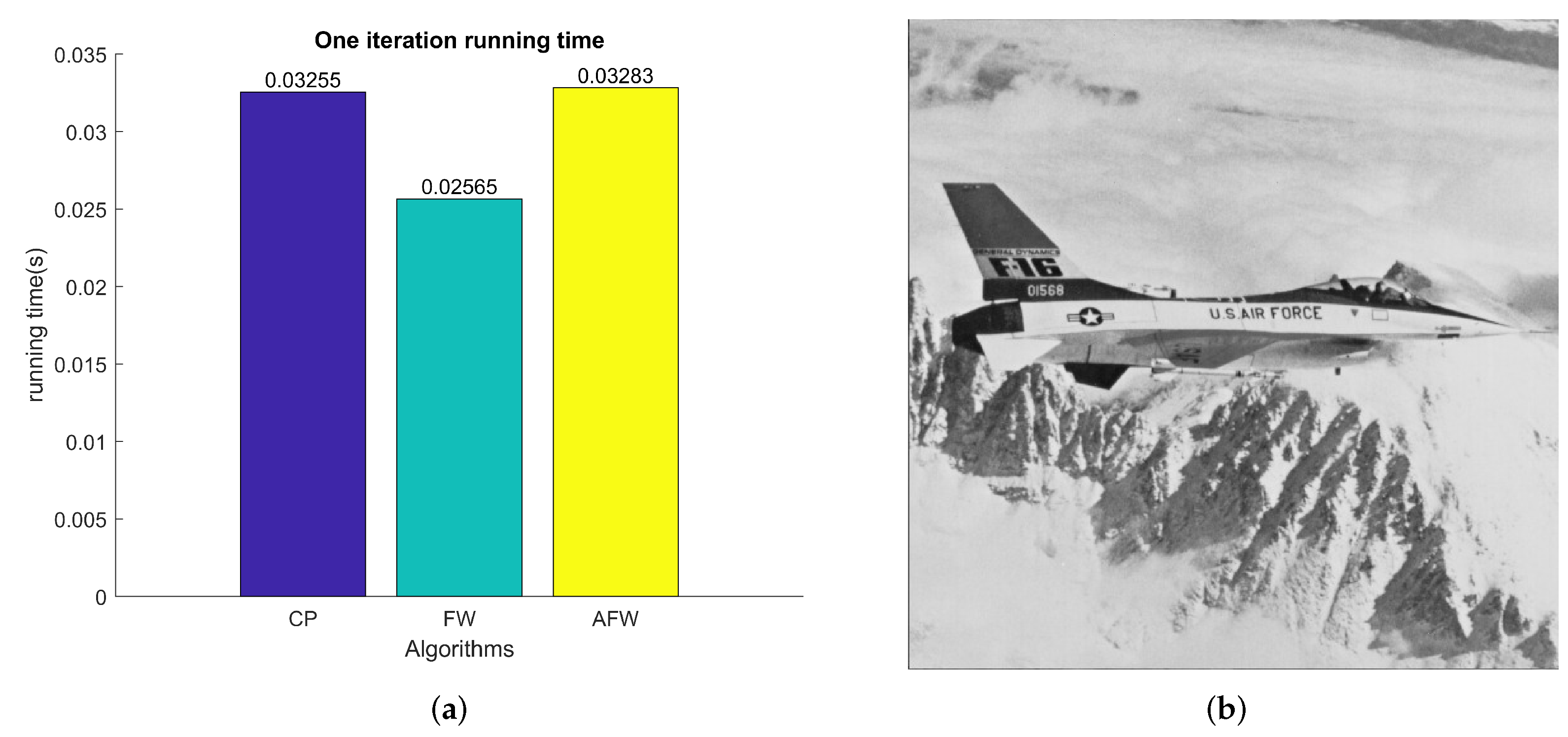
In order to highlight a lower computation cost of the accelerated Chambolle projection, we test one iteration running time on a large image “Airplane”, with a size of 512 × 512 . The result can be seen in Figure 3a.
One iteration running time of CP–FW is the smallest. The running time of CP–AFW is similar to CP, but the formula of algorithms of CP–FW and CP–AFW is simpler than CP. Meanwhile, CP–AFW converges faster than CP. Thus, CP–FW and CP–AFW are superior to CP in the total computation cost.

5.2. Test Algorithms on Dataset

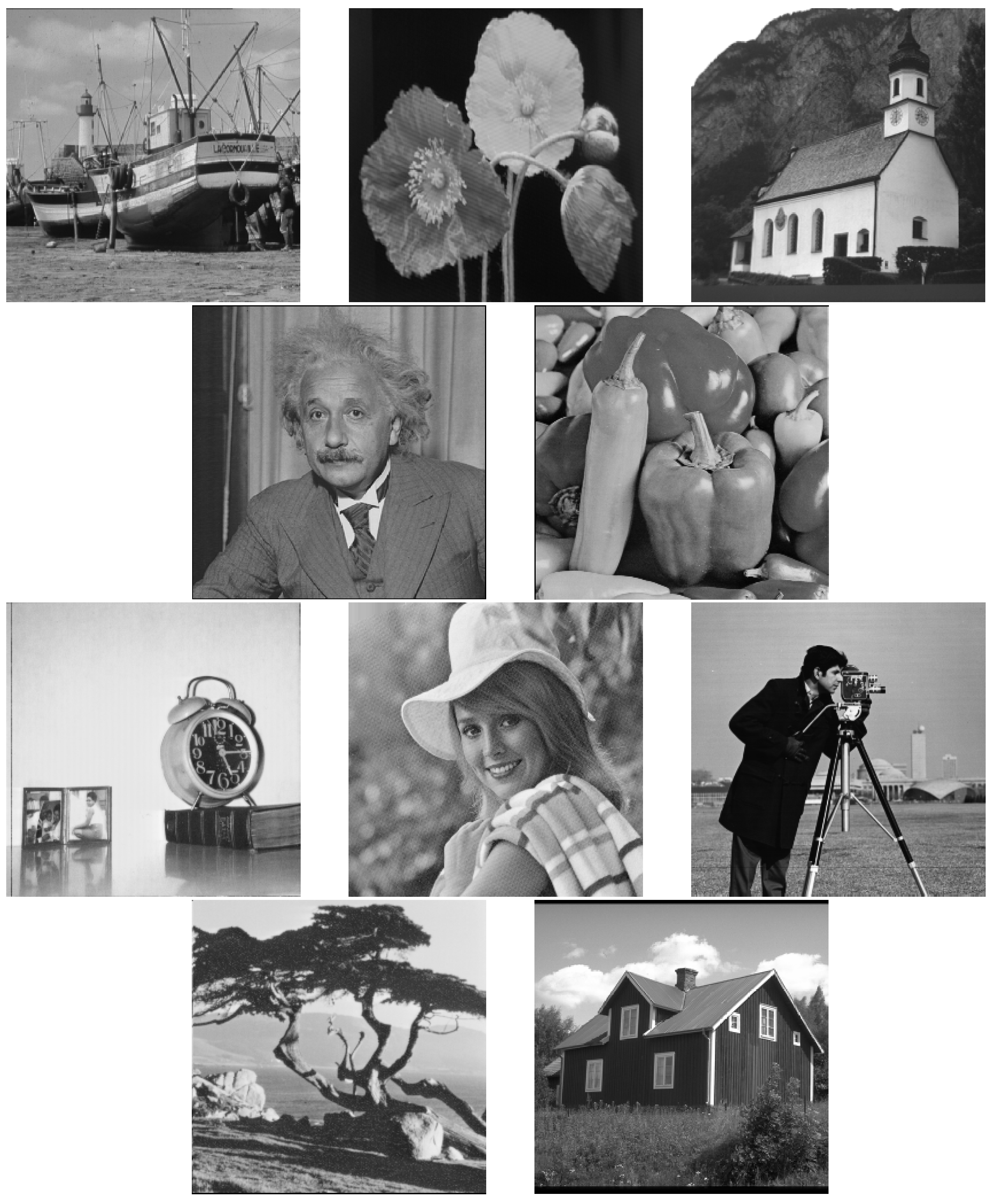
Next, we make a small image dataset for testing all of the algorithms for Gaussian denoising and Poisson denoising in image processing. The dataset includes 10 images, with a size of 256 × 256 pixels. We compare algorithms from the indexes of running time, PSNR and SSIM.
The small image dataset is shown as Figure 4.
We apply algorithms for Gaussian denoising and Poisson denoising to the dataset. The experimental data can be seen in Figure 5 and Figure 6. It is worth noting that the average PSNR of the dataset with the Gaussian noise is 22.2906 dB and the average SSIM is 0.3560. The average PSNR of the dataset with the Poisson noise is 26.4548 dB and the average SSIM is 0.5035.
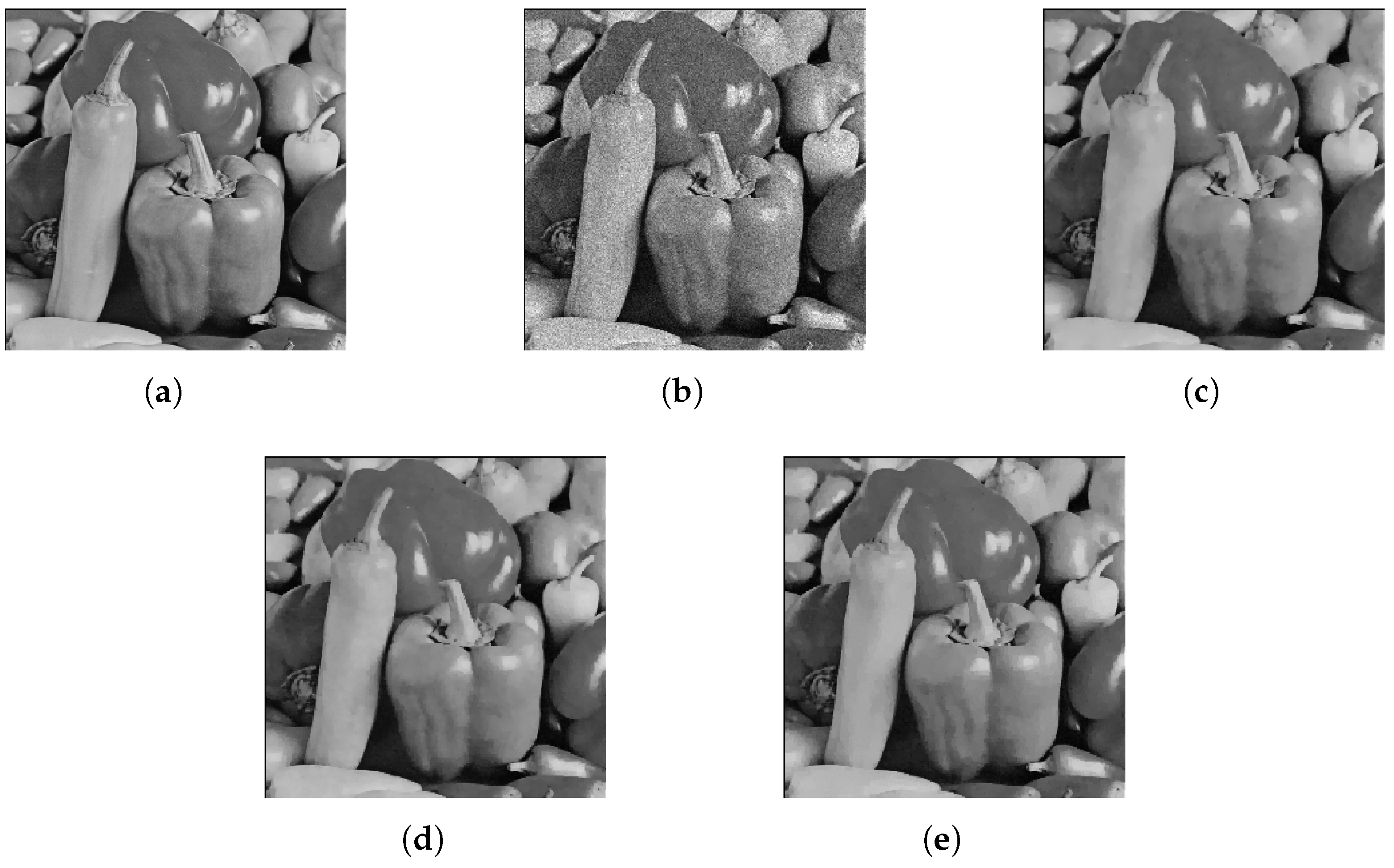
From Figure 5 and Figure 6, the relationship of the running time of all algorithms is shown: CP > CP–FW > CP–AFW. That is, CP has the longest running time on the dataset. The relationship of the PSNR of the algorithms is shown: CP > CP–FW > CP–AFW, and the relationship of SSIM of algorithms is also shown: CP > CP–FW > CP–AFW. Meanwhile, we observe that the index of the PSNR value is similar, but SSIM is not. The SSIM value of CP–FW is similar to CP, but CP–AFW is smaller than the other algorithms, which means that the CP–AFW algorithm for solving the minimizing energy functional for denoising may lose image structural information. In conclusion, CP has a high calculation cost and an excellent denoising performance, but CP–AFW has a low calculation cost and slightly poorer denoising performance than CP. CP–FW is a good algorithm to recommend. We take an image “Papav” from the dataset to show the performance of Gaussian denoising with different algorithms in Figure 7 and the image “Peppers” to show the performance of Poisson denoising in Figure 8. The experiments show that the new accelerated Chambolle algorithms have better trade-off between the computational cost and denoising.

6. Conclusions

Along with the work of the Chambolle projection algorithm for Gaussian denoising, we have proposed the accelerated Chambolle projection based on the Frank–Wolfe method. New algorithms have a lower computation cost and can maintain their denoising performance while reducing computational complexity in image processing. When extending the Chambolle projection algorithm to the Poisson noise condition, as a matter of course, the accelerated Chambolle projection algorithms are also extended. The convergence of algorithms is proved under the Gaussian noise or the Poisson noise condition. Theory and experiments have shown that the new algorithms demonstrate practicability on the task of image processing. It is worth noting that our proposed algorithms can extend to other variant total variation models and other image-processing tasks, which is something we will implement as soon as possible.

Author Contributions

Conceptualization, W.W. and X.F.; methodology, W.W. and X.F.; software, W.W.; validation, W.W.; formal analysis, W.W.; writing—original draft preparation, W.W.; writing—review and editing, W.W. and X.F.; visualization, W.W.; supervision, X.F.; and funding acquisition, W.W. All authors have read and agreed to the published version of the manuscript.

Funding

This research was funded by the National Natural Science Foundation of China grant number 61772389.

Data Availability Statement

Publicly available datasets were analyzed in this study. Our image dataset includes set 12 and publicly available images.

Acknowledgments

The authors would like to thank the National Natural Science Foundation of China (Grants 61772389) for supporting this research work.

Conflicts of Interest

The authors declare no conflict of interest.

References

  1. Wang, Y.; Yang, J.; Yin, W.; Zhang, Y. A new alternating minimization algorithm for total variation image reconstruction. SIAM J. Imaging Sci. 2008, 1, 248–272. [Google Scholar] [CrossRef]
  2. Chambolle, A.; Caselles, V.; Cremers, D.; Novaga, M.; Pock, T. An Introduction to Total Variation for Image Analysis. In Theoretical Foundations and Numerical Methods for Sparse Recovery; Fornasier, M., Ed.; De Gruyter: Berlin, Germany; De Gruyter: New York, NY, USA, 2010; pp. 263–340. [Google Scholar]
  3. Beck, A.; Teboulle, M. Fast Gradient-Based Algorithms for Constrained Total Variation Image Denoising and Deblurring Problems. IEEE Trans. Image Process. 2009, 18, 2419–2434. [Google Scholar] [CrossRef] [Green Version]
  4. Chambolle, A. An Algorithm for Total Variation Minimization and Applications. J. Math. Imaging Vis. 2004, 20, 89–97. [Google Scholar]
  5. Zhou, L.; Tang, J. Fraction-order total variation blind image restoration based on L1-norm. Appl. Math. Model. 2017, 51, 469–476. [Google Scholar] [CrossRef]
  6. Yang, J.H.; Zhao, X.L.; Mei, J.J.; Wang, S.; Ma, T.H.; Huang, T.Z. Total variation and high-order total variation adaptive model for restoring blurred images with Cauchy noise. Comput. Math. Appl. 2019, 77, 1255–1272. [Google Scholar] [CrossRef]
  7. Bayram, I.; Kamasak, M.E. Directional Total Variation. IEEE Signal Process. Lett. 2012, 19, 781–784. [Google Scholar] [CrossRef] [Green Version]
  8. Bredies, K.; Kunisch, K.; Pock, T. Total Generalized Variation. SIAM J. Imaging Sci. 2010, 3, 492–526. [Google Scholar] [CrossRef] [Green Version]
  9. Asaki, T.J.; Le, T.; Chartrand, R. A variational approach to reconstructing images corrupted by poisson noise. J. Math. Imaging Vis. 2007, 27, 257–263. [Google Scholar]
  10. Wang, W.; He, C. A fast and effective method for a Poisson denoising model with total variation. IEEE Singal Process. Lett. 2017, 24, 269–273. [Google Scholar] [CrossRef] [Green Version]
  11. Rahman Chowdhury, M.; Zhang, J.; Qin, J.; Lou, Y. Poisson image denoising based on fractional-order total variation. Inverse Probl. Imaging 2020, 14, 77–96. [Google Scholar] [CrossRef] [Green Version]
  12. Sawatzky, A.; Brune, C.; Koesters, T.; Wuebbeling, F.; Burger, M. EM-TV Methods for Inverse Problems with Poisson Noise. In Level Set and PDE Based Reconstruction Methods in Imaging; Springer: Cham, Switzerland, 2013. [Google Scholar]
  13. Parikh, N.; Boyd, S. Proximal Algorithms. Found. Trends Optim. 2014, 1, 127–239. [Google Scholar] [CrossRef]
  14. Zhang, B.; Zhu, Z.; Luo, Z. A modified Chambolle-Pock primal-dual algorithm for Poisson noise removal. Calcolo 2020, 57, 28. [Google Scholar] [CrossRef]
  15. Jiang, L.; Huang, J.; Lv, X.-G.; Liu, J. Alternating direction method for the high-order total variation-based Poisson noise removal problem. Numer. Algorithms 2015, 69, 495–516. [Google Scholar] [CrossRef]
  16. Wen, Y.; Chan, R.H.; Zeng, T. Primal-dual algorithms for total variation based image restoration under Poisson noise. Sci. China Math. 2016, 59, 141–160. [Google Scholar] [CrossRef]
  17. Zhang, J.; Duan, Y.; Lu, Y.; Ng, M.K.; Chang, H. Bilinear constraint based ADMM for mixed Poisson-Gaussian noise removal. Inverse Probl. Imaging 2020, 15, 1–28. [Google Scholar] [CrossRef]
  18. Rudin, L.I.; Osher, S.; Fatemi, E. Nonlinear total variation based noise removal algorithms. Phys. D Nonlinear Phenom. 1992, 60, 259–268. [Google Scholar] [CrossRef]
  19. Marguerite, F.; Wolfe, P. An algorithm for quadratic programming. Nav. Res. Logist. Q. 1956, 3, 95–110. [Google Scholar]
  20. Jaggi, M. Revisiting Frank–Wolfe: Projection-Free Sparse Convex Optimization. In Proceedings of the 30th International Conference on Machine Learning, Atlanta, GA, USA, 16–21 June 2013. [Google Scholar]
  21. Li, B.; Coutiño, M.; Giannakis, G.B.; Leus, G. A Momentum-Guided Frank–Wolfe Algorithm. IEEE Trans. Signal Process. 2021, 69, 3597–3611. [Google Scholar] [CrossRef]
  22. Salmon, J.; Harmany, Z.; Deledalle, C.A.; Willett, R. Poisson Noise Reduction with Non-local PCA. J. Math. Imaging Vis. 2014, 48, 279–294. [Google Scholar] [CrossRef] [Green Version]
  23. Bindilatti, A.A.; Mascarenhas, N.D.A. A Nonlocal Poisson Denoising Algorithm Based on Stochastic Distances. IEEE Signal Process. Lett. 2013, 20, 1010–1013. [Google Scholar] [CrossRef]
  24. Marais, W.; Willett, R. Proximal-Gradient methods for poisson image reconstruction with BM3D-Based regularization. In Proceedings of the 2017 IEEE 7th International Workshop on Computational Advances in Multi-Sensor Adaptive Processing (CAMSAP), Curacao, The Netherlands, 10–13 December 2017. [Google Scholar]
  25. Azzari, L.; Foi, A. Variance stabilization for noisy + estimate combination in iterative poisson denoising. IEEE Signal Process. Lett. 2016, 23, 1086–1090. [Google Scholar] [CrossRef]
  26. Mäkitalo, M.; Foi, A. Poisson-gaussian denoising using the exact unbiased inverse of the generalized anscombe transformation. In Proceedings of the 2012 IEEE International Conference on Acoustics, Speech and Signal Processing (ICASSP), Kyoto, Japan, 25–30 March 2012; pp. 1081–1084. [Google Scholar]
  27. Makitalo, M.; Foi, A. Optimal Inversion of the Generalized Anscombe Transformation for Poisson-Gaussian Noise. IEEE Trans. Image Process. 2013, 22, 91–103. [Google Scholar] [CrossRef]
  28. Chang, H.; Lou, Y.; Duan, Y.; Marchesini, S. Total Variation–Based Phase Retrieval for Poisson Noise Removal. SIAM J. Imaging Sci. 2018, 11, 24–45. [Google Scholar] [CrossRef]
  29. di Serafino, D.; Pragliola, M. Automatic parameter selection for the TGV regularizer in image restoration under Poisson noise. arXiv 2022, arXiv:2205.13439. [Google Scholar]
  30. Lv, X.G.; Jiang, L.; Liu, J. Deblurring Poisson noisy images by total variation with overlapping group sparsity. Appl. Math. Comput. 2016, 289, 132–148. [Google Scholar] [CrossRef]
  31. Zhang, M.; Zhang, F.; Liu, Q.; Wang, S. VST-Net: Variance-stabilizing Transformation Inspired Network for Poisson Denoising. J. Vis. Commun. Image Represent. 2019, 62, 12–22. [Google Scholar] [CrossRef]
  32. Kumwilaisak, W.; Piriyatharawet, T.; Lasang, P.; Thatphithakkul, N. Image denoising with deep convolutional neural and multi-directional long short-term memory networks under Poisson noise environments. IEEE Access 2020, 8, 86998–87010. [Google Scholar] [CrossRef]
  33. Bauschke, H.H.; Combettes, P.L. Convex Analysis and Monotone Operator Theory in Hilbert Spaces; CMS Books in Mathematics; Springer: New York, NY, USA, 2011. [Google Scholar]
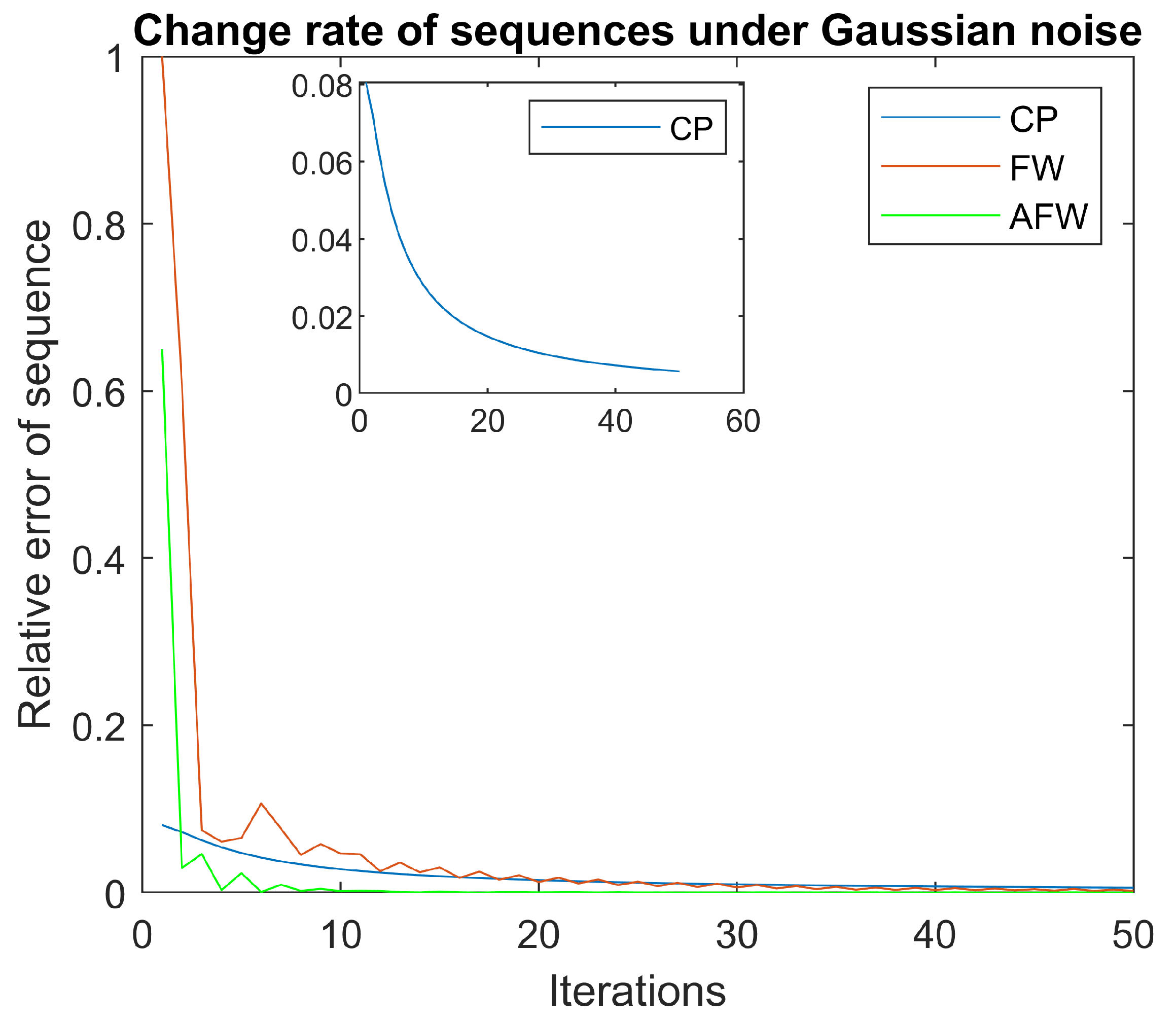
Figure 1. The change rate of sequences under the Gaussian noise condition.
Electronics 11 03751 g001
Figure 2. The change rate of sequences and the change of value of energy functional under the Poisson noise condition. (a) The change rate of sequences; (b) the change of the value of E(u) energy function with iterations.
Electronics 11 03751 g002
Figure 3. Running time. (a) One iteration running time of three algorithms; (b) airplane.
Electronics 11 03751 g003
Figure 4. Image dataset.
Electronics 11 03751 g004
Figure 5. Algorithms of comparation for Gaussian denoising. (a) Running time; (b) the average PSNR of dataset for Gaussian denoising; and (c) the average SSIM of dataset for Gaussian denoising.
Electronics 11 03751 g005
Figure 6. Algorithms of comparation for Poisson denoising. (a) Running time; (b) the average PSNR of dataset for Poisson denoising; and (c) the average SSIM of dataset for Poisson denoising.
Electronics 11 03751 g006
Figure 7. Papav. (a) Original image; (b) Gaussian noise image; (c) CP for denoising; (d) CP–FW for denoising; and (e) CP–AFW for denoising.
Electronics 11 03751 g007
Figure 8. Peppers. (a) Original image; (b) Poisson noise image; (c) CP for denoising; (d) CP–FW for denoising; and (e) CP–AFW for denoising.
Electronics 11 03751 g008
Publisher’s Note: MDPI stays neutral with regard to jurisdictional claims in published maps and institutional affiliations.