Participation of Electric Vehicles in a Delay-Dependent Stability Analysis of LFC Considering Demand Response Control

Abstract

Today, time-varying delays may result from a communication network’s engagement in frequency control services. These delays have an impact on the effectiveness of the load frequency control (LFC) system, which can occasionally lead to power system instability. The electric vehicle (EV) can be used as a beneficial source for the LFC system with the development of demand-side response due to its vehicle-to-grid capacity. Although demand response control has certain advantages for the power system, communication networks used in LFC systems result in time delays that reduce the stability of the LFC schemes. A stability study of an LFC system, comprising an EV aggregator with two additive time-varying delays, is demonstrated in this work. An enhanced Lyapunov–Krasovskii functional (LKF), which incorporates time-varying delays using the linear matrix inequality approach, is used to perform a delay-dependent stability analysis of the LFC to determine the stability zone and criterion. In conclusion, the efficiency of the proposed stability criterion is validated by making use of the thorough simulation findings.

1. Introduction

Time delays will inevitably occur in communication channels when a growing number of closed-loop systems are implemented using communication networks. It is generally understood that the presence of time delay in a dynamical system frequently leads to a decrease in system stability and performance. The operation of the smart electrical system may be impacted by communication delays, which could result in power losses and frequency variation. It is crucial to look into the sources of these issues and the potential mitigation methods. Due to the significant worldwide contribution of conventional vehicles to CO₂ emissions, electric vehicles (EVs) have drawn a lot of interest. This has raised the possibility that EV power generation could improve the reliability of the energy supply. For instance, the vehicle-to-grid (V2G) concept enables vehicles to return stored energy during their idling time to the grid during peak demand periods, thereby enhancing the operation of power systems [1]. The framework of the traditional load frequency control (LFC) system has been enhanced [2] due to the widespread use of EVs in current networks and their significant potential to contribute to markets for ancillary services. As a result, it is important to take into account the delay-based stability of the LFC, which includes the EV aggregator. This literature review starts with a brief analysis of the works that discuss how EVs affect ancillary services. The effect of time-varying delays in EV aggregators on frequency regulation is then studied.

V2G is crucial to the 21st-century electric grid, which is based on renewable energy sources, as described in [3]. Bidirectional power flows can result from using EV batteries for frequency control [4]. A technology that has promise for the future operation of the power system is the use of EVs [5]. Compared with traditional generators, EV batteries can interchange electricity with the network more quickly. Thus, taking EVs into account improves the LFC system’s dynamic stability. EV aggregators serve as the user interface between residential customers and the operator of the autonomous system. EV aggregators function for the autonomous system operator as a big portion of the generation or load, both of which can be utilized in auxiliary services in a controlled manner. Ref. [6] investigated and analyzed the problem of stability in aperiodic-sampled data control systems with a time delay. The improvement of system performance in attendance with a time delay is a surprising phenomenon that can be obtained theoretically. However, in real-world applications, time delays are a ubiquitous occurrence that, depending on the circumstances, can either severely reduce the system’s performance or even cause it to become unstable. It should be noted that a frequency control service that takes into account the EV’s aggregator could result in a delay that varies in time in LFC schemes. The LFC frequency control system performance is affected by these delays. In some circumstances, insufficient consideration of time-varying delays leads to power system instability. Since delays have an impact on frequency regulation performance. Ref. [7] expanded the traditional LFC model by incorporating numerous EV aggregators with different delay characteristics. In automatic generation control, communication networks send control instructions to EVs. The dedicated open network determines the type of access to communication networks. The apparent relationship between cost and price in the open communication network is used to calculate the access rate to communication resources. The stability of time-delayed LFC systems involves the calculation of the delay margin and the configuration of the controller’s parameters. The maximum amount of time delay that a system can withstand before becoming unstable is known as the delay margin. Theoretical delay margins are calculated for a variety of controller gains, and simulation studies are used to confirm their accuracy.

A delay-based stability analysis of frequency control was conducted in [8]. For large-scale power systems, precise delay margins can be calculated using an efficient method, provided in [9]. A delay-based stability analysis of networked LFC systems in single and multi-area power systems was investigated and analyzed in [10]. One of the methods for analyzing the stability of time-varying delay systems was the delay-dependent matrix-based estimate methodology. The less conservative stability criteria in linear matrix inequality (LMI) could be met by the estimate approach [7]. Delay-dependent LMI-based stability analysis approaches have been primarily used for delayed LFC systems. These techniques are frequently employed in stability studies of time-delayed LFC systems and have produced outstanding outcomes. To enhance the numerical tractability of delay-dependent stability, Ref. [11] presented the chordal sparsity and symmetry of an LFC loop graph. In [12], the authors demonstrated how to construct a criterion for assessing the delay-dependent stability of a multi-area scheme that contains unknown and time-varying load oscillation. This was accomplished by analyzing the relationship between the delay and the stability.

As seen in [13], the conservatism of the hierarchy stability criterion could be reduced by using multiple integral approaches and the free-weighting matrix technique. Ref. [14] researched ways to assess the stability of the microgrid in the presence of plug-in electric vehicles and communication delays. The performance analysis of a multi-area decentralized LFC with time-varying delays was presented in [15]. In another study, an augmented LKF was proposed to survey the stability of power systems with PI-based LFC systems in the presence of time-varying delays [16]. The authors of [17] investigated a decentralized frequency control based on a switching strategy, improving the stability in power mismatch and communication change. In [18], the quadratic function, with regard to the time-varying delay, was frequently utilized as an analytical tool. The proposed lemma included an adjustable parameter to lower the conservatism; it reduces the popular lemma that is presently used by fixing a parameter as a particular value, and the benefits of the proposed lemma were demonstrated based on a numerical example.

In [19], a fractional-order PI controller for a sample LFC system that takes into consideration time-based delay was developed. To overcome the limitations of conventional controllers, the need for accurate and fast-acting control over an LFC system seems necessary. In order to establish stability criteria and provide a method to increase calculation accuracy and decrease computation time, delay-dependent stability for an LFC system was introduced in [20]. A new rebuilt model for the delayed LFC system taking wind power into account was described in Ref. [21], and it attempts to increase the computational effectiveness of PID controllers while maintaining their dynamic performance.

Using memristor-based coupled neural networks [22] apart from PI and PID controllers could be interesting for researchers. The use of time-varying delays in data transfer and uncertainty in a one-area network was analyzed in [23]. In the research that has been performed on LFC schemes, the problem of delay-dependent stability in terms of obtaining a stability region, which provides the desired efficiency of the system, has not been investigated. Few works in the literature have been produced regarding the control domain, where there are many time-varying delay-dependent stability areas. In an LFC system, new criteria with delay dependencies in terms of LMIs were calculated using the augmented LKF [24]. An augmented Lyapunov function and Wirtinger inequality were presented to maintain a stable condition in a large-scale multi-area LFC scheme with reduced conservatism. This was done to reduce the calculation burden of delay-dependent stability analysis and improve the accuracy of computation [25]. Ref. [26] constructed single and multiple time-varying delays to demonstrate delay margins of an example frequency regulation in the presence of EV aggregators. In addition, a Bessel–Legendre inequality-based LKF, as well as a model reconstruction technique, was proposed and used to analyze the delayed LFC system with EV aggregators [27]. Another challenging issue is how to acquire more precise delay margins with less computational complexity. However, there are few studies examining the interdependence and interaction of LFC systems with time delays.

Table 1. A summary of the literature concerning stability studies of LFC systems with variable delays.

Ref	Methodology	Highlights
[28]	Direct method based on the transcendental term’s removal	- Stability analysis and delay margin calculation for various PI controller gains and participation factor ratios; - Validation of stability delay margin accuracy using a root approach based on quasi-polynomial mapping.
[29]	Lyapunov theorem and LMI	- A discrete-time LFC model with time delay;- Using matrix uncertainty to investigate the effect of time-varying delays; - Suggesting a stability criterion for the LFC system with multiple time-varying delays using the region–division approach; - The development of a heuristic method in order to locate an appropriate division for the proposed stability criterion.
[30]	Simple LKF and integral inequalities	- Considering the nonlinearly perturbed and random disturbance of system parameters; - Taking into account unknown exogenous load disturbance and random system parameter disturbance; - Analyzing the relationship between time delay variation rates, load disturbance levels, PI controller gains, and LFC system delay margins.
[31]	Critical eigenvalues on the imaginary axis	- The investigation of the effect of incommensurate time delays on the multi-area LFC systems; - Computation of stability delay margins for multi-area LFC systems using the eigenvalue tracing method; - A comprehensive stability analysis of the multi-area LFC system using the eigenvalue tracing approach.
[32]	Wirtinger-based improved inequality; bounding lemma and LMI techniques	- Evaluating time-varying delays based on LFC system stability with EV aggregators; - Calculating stability zones and criteria using LMI and Lyapunov–Krasovskii theory; - Investigating the participation ratio of the EV aggregators in the maximum permitted delay.
[33]	Nonlinear equation solving	- Examining the influence of PI controller gains and system parameters on the delay margin using sensitivity analysis; - Presenting the stability region of the LFC system; - Studying the influence of the system parameters on the stability region.
[34]	Lyapunov–Krasovskii plus LMI	- Integrating wind energy and electric vehicles into a single-area LFC system with time-varying delay; - The proposal of two new stability criteria for the LFC model, which can either include or exclude uncertain parameters; - Obtaining a less conservative maximum permitted delay for the LFC system.

is a summary of publications that were recently published on the subject of stability in time-delayed LFC systems.

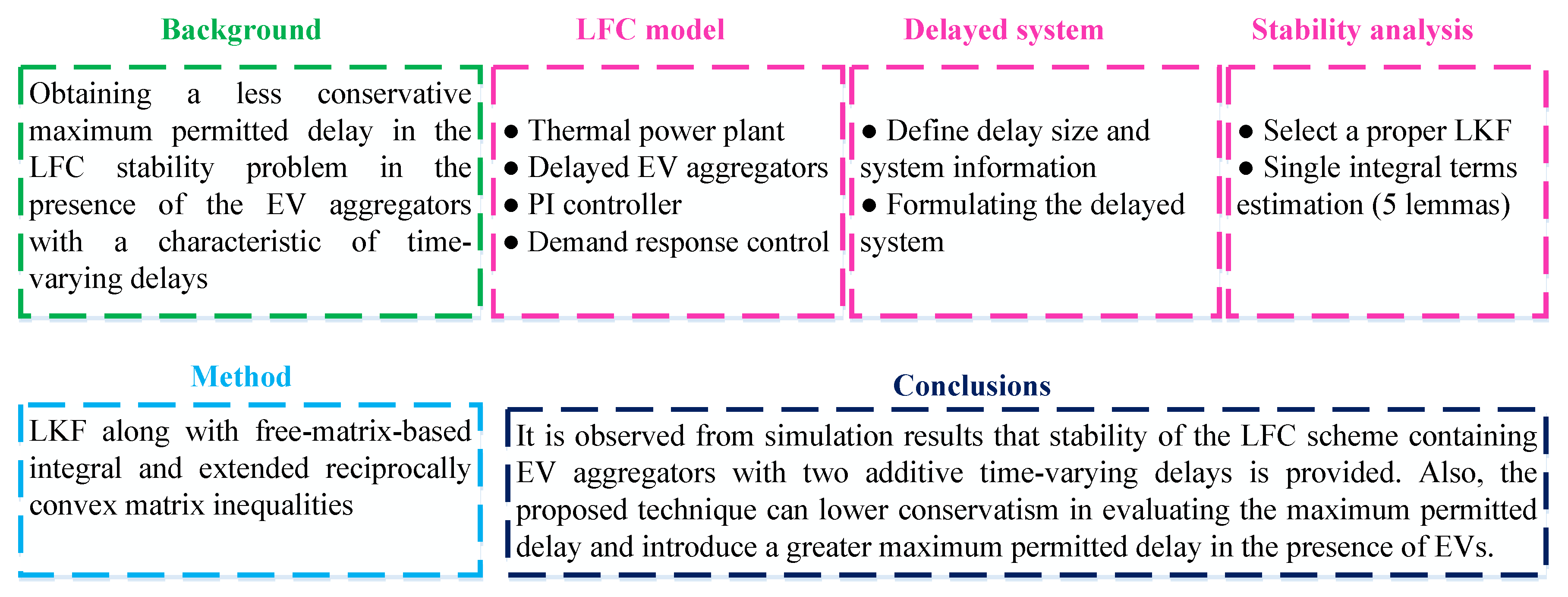
Regarding the aforementioned information, our work is driven by the necessity of reducing conservatism in the largest permitted delay computation, given that the LFC stability problem, combined with EV aggregator participation in frequency control, exhibits time-varying delays. The most significant contributions of this work can be described as follows:

• The calculation of the stability regions and criteria with an improved delay interconnection LKF.
• Using extended reciprocally convex matrix (ERCM) inequalities and a free-matrix-based integral (FMBI) to yield the upper bound of the derivative of the proposed LKF.
• Investigating the various impacts of the EV aggregator participation ratio, with and without demand response (DR) control, on the maximum permitted delay.

The remainder of the paper will be presented below. In Section 2, an LFC system with a delayed EV aggregator is described. In Section 3, the stability analysis is studied. The findings of the simulation are presented in Section 4, and the paper is concluded in Section 5.

2. LFC System Model with Delayed EV Aggregator

It is expected that EV aggregators will be able to provide frequency control services by employing the available EVs. Consequently, the control center transmits directives to EV aggregators to eliminate power fluctuations. Then, once the command has been received, the amount of contribution that each EV brings to the table in terms of engaging in frequency control is calculated. Be aware that there is a time delay involved whenever data are transferred across a communication network. As a result, the response time of each EV will be delayed. For the purposes of investigating small-signal stability, it is necessary to construct a linearized dynamic model of all system components. In a number of studies, many types of typical LFC systems were introduced. A delay-dependent stability analysis of the LFC system is shown in a general form in Figure 1. Figure 2 depicts a one-area LFC method that considers multiple EV aggregators with time-varying delays.

The participation ratios ${\alpha }_1,{\alpha }_2,\dots \hspace{0.17em}and\hspace{0.17em}{\alpha }_N$ show the contribution of each EV aggregator to the frequency control service, while the participation ratio, ${\alpha }_0$, shows the contribution of the generator. The PI controller is chosen for frequency control in the LFC scheme due to its useful applications in a variety of real systems. The synchronous generator and N numbers of the EV aggregators receive control orders from the PI controller. It is important to note the total of the contributory components.

2.1. Thermal Power Plant Model

By utilizing various power control techniques, the synchronous generator can instantaneously detect load variations [35]. The generator adjusts both the amount of fuel it uses and the amount of electricity it produces in response to changes in the load demand. It is important to take note that the governor is connected to the synchronous generators.

2.2. Delayed EV Aggregator Model

The integration of the EV battery into the LFC strategy results in a significant increase in the performance of the system. In many instances [36], the mathematical model of the EV battery is presented in the form of a first-order transfer function. In Figure 2, $e^{-s\tau (t)}$ represents the delay in command transmission from the EV aggregator. The term $\tau (t)$ refers to the variable delay that occurs during the transfer of data from an open communication network. An equivalent model of an electric vehicle aggregator may be developed by using a single delay function under the assumption that all EVs have the same delay characteristic and time constant. The following equation should be used for the computation of the single-area LFC system with N units of EV aggregator:

$$\begin{array}{l}\Delta \dot{f}=\frac{-D}{M}\Delta f+\frac{1}{M}\Delta P_g+\frac{1}{M}\Delta P_{\mathrm{EV},1}+\dots +\frac{1}{M}\Delta P_{\mathrm{EV},N}+\frac{1}{M}\Delta P_{\mathrm{EV},1}(t-{\tau }_{1j}(t))+\dots +\frac{1}{M}\Delta P_{\mathrm{EV},N}(t-{\tau }_{Nj}(t))-\frac{1}{M}\Delta P_d\\ \Delta {\dot{X}}_g=\frac{-1}{R{T}_g}\Delta f-\frac{1}{T_g}\Delta X_g+\frac{{\alpha }_0}{T_g}u(t)\\ \Delta {\dot{P}}_m=\frac{-F_p}{R{T}_g}\Delta f+\frac{T_g-F_p{T}_r}{T_r{T}_g}\Delta X_g-\frac{1}{T_r}\Delta P_m+\frac{F_p{\alpha }_0}{T_g}u(t)\\ \Delta {\dot{P}}_g=\frac{1}{T_c}\Delta P_m-\frac{1}{T_c}\Delta P_g\\ \Delta {\dot{P}}_{\mathrm{EV},1}=\frac{-1}{T_{\mathrm{EV},1}}\Delta P_{\mathrm{EV},1}+\frac{{\alpha }_1{K}_{\mathrm{EV},1}}{T_{\mathrm{EV},1}}u(t-{\tau }_{1i}(t))\hspace{1em}\hspace{1em}\dots \\ \Delta {\dot{P}}_{\mathrm{EV},N}=\frac{-1}{T_{\mathrm{EV},N}}\Delta P_{\mathrm{EV},N}+\frac{{\alpha }_N{K}_{\mathrm{EV},N}}{T_{\mathrm{EV},N}}u(t-{\tau }_{Ni}(t)) \\ \mathrm{y}=\beta \Delta f\end{array}$$

(1)

where $\Delta f,\hspace{0.17em}\hspace{0.17em}\Delta X_g,\hspace{0.17em}\hspace{0.17em}\Delta P_m,\hspace{0.17em}\hspace{0.17em}\Delta P_g$ and $\Delta P_{\mathrm{EV},i}$ are variations in frequency, valve position, mechanical, generator output powers, and ith EV aggregator electric power, respectively. In addition, $\beta$ is the frequency bias factor, $u(t)$ is the controller output, and $R$ is the speed regulation factor.

2.3. Demand Response Control

DR control is defined as a demand-side deviation from normal power consumption patterns. DR may provide various services in the modern era of power systems and be effectively used for quick frequency control and long-term energy balance. When a negative or positive frequency variation necessitates decreasing or increasing responsive loads, the employment of DR for frequency control is straightforward to comprehend. Today’s electric power system could have a higher penetration of controllable loads due to DR controls, EV aggregators, and renewable energy resources with diverse storage systems. Note that the DR involves shifting or shedding electricity demand to provide flexibility in wholesale and ancillary power markets, helping to balance the grid [37]. It can be seen from Figure 2 that the frequency deviation will not be zero unless the supplementary and DR controls exist. In addition, DR provides an extra degree of freedom for system frequency regulation. With DR and EV aggregators available in the LFC, the frequency deviation will be zero at a steady state if

$$\Delta f(s)=\frac{\Delta P_g(s)+\Delta P_{\mathrm{EV}}(s)+\Delta P_{\mathrm{DR}}(s)-\Delta P_d(s)}{D+\frac{1}{M}}=0$$

(2)

As a result of the integration of the DR control into the LFC system, the necessary amount of control effort is shared between the primary loops, EV aggregators, and the DR control in the following equation:

$$\begin{array}{l}\Delta P_g(s)={\alpha }_0\Delta P_d\\ \Delta P_{\mathrm{EV}}(s)={\alpha }_1\Delta P_d\\ \Delta P_{\mathrm{DR}}(s)={\alpha }_2\Delta P_d\end{array}$$

(3)

where ${\alpha }_0+{\alpha }_1+{\alpha }_2=1$.

3. Analysis of Delayed System Stability

In order to determine the area of the system in which stability may be maintained, it is necessary to take into consideration the effects of temporal delays and conduct a stability analysis known as a delay-dependent stability analysis. The delay size and knowledge of the system both have a role in the delayed system’s stability. The strong stabilization of the delayed system is accomplished using the delay-dependent stability technique. It should be noted that this delay margin calculation theorem is conservative. Therefore, the Lyapunov–Krasovskii theorem is proposed since it is less conservative than other alternatives. The level of conservatism in the system stability analysis may be lowered by using the LMI framework to choose an appropriate Lyapunov–Krasovskii theorem that limits inequality.

It is commonly recognized that time delay is a key cause of instability and poor performance in many practical systems, such as communication networks and economic systems. Since the characteristics of the two delays may not be similar due to network conditions, it is unreasonable to combine them. Thus, the closed-loop system can be described as follows [38,39]:

$$\dot{x}(t)=Ax(t)+A_{d}x (t-{\tau }_1(t)-{\tau }_2(t))$$

(4)

$$\begin{array}{l}x(t)=\varphi (t) , t\in [-{\tau }^M,0]\\ 0\le {\tau }_1(t)\le {\tau }_1{}^M, {\dot{\tau }}_1(t)\le u_1\\ 0\le {\tau }_2(t)\le {\tau }_2{}^M, {\dot{\tau }}_2(t)\le u_2\end{array}$$

(5)

where $x(t),\hspace{0.17em}\hspace{0.17em}A$ and $A_d$ are the system state vector, state coefficient matrix, and constant matrix, respectively. ${\tau }_1(t)$ and ${\tau }_2(t)$ indicate two additive delay components that are cumulative in the state. The terms ${\tau }_{{}_1}^M$ and ${\tau }_2^M$ are exploited to show the upper bound of ${\tau }_1(t)$ and ${\tau }_2(t)$, respectively. Let ${\tau }^M={\tau }_1^M+{\tau }_2^M$, $u=u_1+u_2$, and $\tau (t)={\tau }_1(t)+{\tau }_2(t)$. The $\varphi (t)$ is a continuously differentiable function. The PI controller is transformed into an output feedback problem before using the proposed theorem [40]. Through the utilization of this transformation, the closed-loop state-space model can be derived as:

$$X(t)={\left[\begin{array}{cc}{x}^T& {\displaystyle \int y^T}\end{array}\right]}^T,Y(t)={\left[\begin{array}{cc}{y}^T& {\displaystyle \int y^T}\end{array}\right]}^T$$

(6)

$$\begin{array}{l}\dot{X}(t)=A_{0}X(t)+A_{d}X (t-{\tau }_1(t)-{\tau }_2(t))\\ Y(t)=CX(t)\end{array}$$

(7)

where

$$A_0=\left[\begin{array}{cc}A& 0\\ c& 0\end{array}\right],\hspace{0.17em}\hspace{0.17em}B=\left[\begin{array}{c}b+b_k\\ 0\end{array}\right],\hspace{0.17em}\hspace{0.17em}C=\left[\begin{array}{cc}c& 0\\ 0& 1\end{array}\right],\hspace{0.17em}\hspace{0.17em}{A}_d=-BKC$$

where $b,\hspace{0.17em}\hspace{0.17em}{b}_k$ and $c$ are the constant coefficients. ${\tau }^M$ is the maximum permitted delay for a single EV’s aggregator. In the following, FMBI and ERCM inequalities can be utilized to estimate the single integral terms.

Lemma 1: 

Let $X$be a differentiable signal in$[\alpha ,\beta ]\to {\Re }^n$for a positive definite matrix,$R\in {\Re }^{n\times n}$; the following inequality can be satisfied [41]:

$$(\beta -\alpha ){\displaystyle {\int }_{\alpha }^{\beta }{x}^T(s)Rx(s)ds\ge {\left({\displaystyle {\int }_{\alpha }^{\beta }x(s)ds}\right)}^{T}R\left({\displaystyle {\int }_{\alpha }^{\beta }x(s)ds}\right)}$$

(8)

$$\frac{{(\beta -\alpha )}^2}{2}{\displaystyle {\int }_{\alpha }^{\beta }{\displaystyle {\int }_{\theta }^{\beta }}{x}^T(s)Rx(s)dsd\theta \ge }{\left({\displaystyle {\int }_{\alpha }^{\beta }{\displaystyle {\int }_{\theta }^{\beta }}x(s)dsd\theta }\right)}^{T}R\left({\displaystyle {\int }_{\alpha }^{\beta }{\displaystyle {\int }_{\theta }^{\beta }}x(s)dsd\theta }\right)$$

(9)

Lemma 2: 

Let$X$be a continuously differentiable signal in$[\alpha ,\beta ]\to {\Re }^n$for a symmetric matrix$R\in {\Re }^{n\times n}>0$; the following inequality can be satisfied [42]:

$${\displaystyle {\int }_{\alpha }^{\beta }{\dot{x}}^T(s)R\dot{x}(s)ds\ge \frac{1}{\beta -\alpha }{\chi }_1^{T}R{\chi }_1}+\frac{3}{\beta -\alpha }{\chi }_2^{T}R{\chi }_2$$

(10)

where

$${\chi }_1=x(\beta )-x(\alpha ),\hspace{0.17em}\hspace{0.17em}\hspace{0.17em}\hspace{0.17em}\hspace{0.17em}\hspace{0.17em}{\chi }_2=x(\beta )+x(\alpha )-\frac{2}{\beta -\alpha }{\displaystyle {\int }_{\alpha }^{\beta }x(s)ds}$$

(11)

Lemma 3: 

Let$X$be a differentiable signal in$[\alpha ,\beta ]\to {\Re }^n$for symmetric matrices ($R\in {\Re }^{n\times n}$and$X,Z\in {\Re }^{3n\times 3n}$) and any matrices ($Y\in {\Re }^{3n\times 3n}$and$N_1,N_2\in {\Re }^{3n\times n}$), thus satisfying the following [43]:

$$\left[\begin{array}{ccc}X& Y& N_1\\ *& Z& N_2\\ *& *& R\end{array}\right]\ge 0$$

(12)

The following inequality can be satisfied:

$$-{\displaystyle {\int }_{\alpha }^{\beta }{\dot{x}}^T(s)R\dot{x}(s)ds\le \hspace{0.17em}}{\varpi }^T\widehat{\Omega }\varpi$$

(13)

where

$$\begin{array}{l}\varpi ={\left[x^T(\beta )\hspace{0.17em}\hspace{0.17em}\hspace{0.17em}{x}^T(\alpha )\hspace{0.17em}\hspace{0.17em}\hspace{0.17em}\frac{1}{\beta -\alpha }{\displaystyle {\int }_{\alpha }^{\beta }{x}^T(s)ds}\right]}^T\\ \widehat{\Omega }=(\beta -\alpha )\left(X+\frac{1}{3}Z\right)+Sym\left\{N_1{\Pi }_1+N_2{\Pi }_2\right\}\\ {\overline{\Pi }}_1={\overline{e}}_1-{\overline{e}}_2,\hspace{0.17em}\hspace{0.17em}\hspace{0.17em}\hspace{0.17em}\hspace{0.17em}{\overline{\Pi }}_2=2{\overline{e}}_3-{\overline{e}}_1-{\overline{e}}_2\\ {\overline{e}}_1=[1\hspace{0.17em}\hspace{0.17em}\hspace{0.17em}0\hspace{0.17em}\hspace{0.17em}\hspace{0.17em}0],\hspace{0.17em}\hspace{0.17em}\hspace{0.17em}\hspace{0.17em}\hspace{0.17em}{\overline{e}}_2=[0\hspace{0.17em}\hspace{0.17em}\hspace{0.17em}1\hspace{0.17em}\hspace{0.17em}\hspace{0.17em}0],\hspace{0.17em}\hspace{0.17em}\hspace{0.17em}\hspace{0.17em}\hspace{0.17em}{\overline{e}}_3=[0\hspace{0.17em}\hspace{0.17em}\hspace{0.17em}0\hspace{0.17em}\hspace{0.17em}\hspace{0.17em}1].\end{array}$$

(14)

Lemma 4: 

For a real scalar$\alpha \in (0,1)$, symmetric matrices$X_1,X_2>0$, and any matrices ($S_1$and$S_2$), the following matrix inequality holds [44]:

$$\left[\begin{array}{cc}\frac{1}{\alpha }{X}_1\hfill & \hfill 0\hfill \\ 0\hfill & \frac{1}{1-\alpha }{X}_2\end{array}\right]\ge \left[\begin{array}{cc}{X}_1+(1-\alpha )T_1\hfill & \hfill (1-\alpha )S_1\hspace{0.17em}+\alpha S_2\hspace{0.17em}\\ *& \hfill X_2+\alpha T_2\end{array}\right]$$

(15)

where $T_1=X_1-S_2{X}_2^{-1}{S}_2^T$ and $T_2=X_2-S_1^T{X}_1^{-1}{S}_1$.

Lemma 5: 

Given the symmetric matrix$S=\left[\begin{array}{cc}{S}_{11}& S_{12}\\ *& S_{22}\end{array}\right]$, where$S_{11}\in {\Re }^{r\times r}$, the following three conditions are equivalent [45]:

$$\begin{array}{l}(i)\hspace{0.17em}\hspace{0.17em}\hspace{0.17em}\hspace{0.17em}\hspace{0.17em}S<0\\ (ii)\hspace{0.17em}\hspace{0.17em}\hspace{0.17em}\hspace{0.17em}{S}_{11}<0,\hspace{0.17em}\hspace{0.17em}\hspace{0.17em}\hspace{0.17em}\hspace{0.17em}{S}_{22}-S_{12}^T{S}_{11}^{-1}{S}_{12}<0\\ (iii)\hspace{0.17em}\hspace{0.17em}\hspace{0.17em}{S}_{22}<0,\hspace{0.17em}\hspace{0.17em}\hspace{0.17em}\hspace{0.17em}{S}_{11}-S_{12}{S}_{22}^{-1}{S}_{12}^T<0\end{array}$$

(16)

According to current research trends, to achieve a less conservative stability criterion, the majority of studies are concentrated on two aspects: the construction of various types of innovative augmented LKFs and the development of more effective mathematical procedures for the derivative of LKFs. The main idea behind these methods is to add more time-delay information to the LKF process. However, this has a drawback where the computing burden increases dramatically as the complexity of the created LKFs and established mathematical approaches increases. Consequently, it appears essential and necessary to identify another plan to reach this objective. As a result, ERCM inequalities and FMBI are exploited to compute the derivative of the proposed LKF. Using the suggested methodology, having more information on the two time-varying delays leads to the obtainment of an improved stability criterion. Therefore, the following notations to avoid the vector and matrix representations are used:

$$\begin{array}{l}{\xi }_1(t)={\left[x^T(t)\hspace{0.17em},{\displaystyle {\int }_{t-\tau }^t{x}^T(s)ds}\hspace{0.17em},{\displaystyle {\int }_{t-{\tau }_2}^{t-{\tau }_1}{x}^T(s)ds}\hspace{0.17em},{\displaystyle {\int }_{t-\tau }^{t-{\tau }_1}{x}^T(s)ds\hspace{0.17em},{\displaystyle {\int }_{t-\tau }^{t-{\tau }_2}{x}^T(s)ds}}\right]}^T\\ {\xi }_2(t)={\left[x^T(t),\hspace{0.17em} x^T(t-{\tau }_1),\hspace{0.17em} x^T(t-{\tau }_2)\hspace{0.17em}, x^T(t-\tau )\hspace{0.17em}, x^T(t-{\tau }_1(t)),\hspace{0.17em} x^T(t-{\tau }_2(t))\right]}^T\\ {\xi }_3(t)={\left[x^T(t-\tau (t))\hspace{0.17em},\hspace{0.17em} \frac{1}{{\tau }_1(t)}{\displaystyle {\int }_{t-{\tau }_1(t)}^t{x}^T(s)ds}, \frac{1}{{\tau }_1-{\tau }_1(t)}{\displaystyle {\int }_{t-{\tau }_1}^{t-{\tau }_1(t)}{x}^T(s)ds}\right]}^T\\ {\xi }_4(t)={\left[\frac{1}{{\tau }_2(t)}{\displaystyle {\int }_{t-{\tau }_2(t)}^t{x}^T(s)ds}, \frac{1}{{\tau }_2-{\tau }_2(t)}{\displaystyle {\int }_{t-{\tau }_2}^{t-{\tau }_2(t)}{x}^T(s)ds, \frac{1}{\tau (t)}{\displaystyle {\int }_{t-\tau (t)}^t{x}^T(s)ds}}\right]}^T\\ {\xi }_5(t)={\left[\begin{array}{l}\frac{1}{{\tau }_2-{\tau }_1}{\displaystyle \underset{t-{\tau }_2}{\overset{t-{\tau }_1}{\int }}{x}^T(s)ds}\hspace{0.17em}, \frac{1}{\tau -\tau (t)}{\displaystyle \underset{t-\tau }{\overset{t-\tau (t)}{\int }}{x}^T(s)ds}, \frac{1}{\tau -{\tau }_1}{\displaystyle \underset{t-\tau }{\overset{t-{\tau }_1}{\int }}{x}^T(s)ds\hspace{0.17em}},\\ \frac{1}{\tau -{\tau }_2}{\displaystyle \underset{t-\tau }{\overset{t-{\tau }_2}{\int }}{x}^T(s)ds}\end{array}\right]}^T\end{array}$$

$$\begin{array}{l}\xi (t)={\left[{\xi }_2(t)\hspace{0.17em}\hspace{0.17em}\hspace{0.17em}{\xi }_3(t)\hspace{0.17em}\hspace{0.17em}\hspace{0.17em}{\xi }_4(t)\hspace{0.17em}\hspace{0.17em}\hspace{0.17em}{\xi }_5(t)\right]}^T\\ e_i={[0_{n\times (i-1)n}\hspace{0.17em}\hspace{0.17em}\hspace{0.17em}{I}_n\hspace{0.17em}\hspace{0.17em}\hspace{0.17em}{0}_{n\times (16-i)n}]}^T,\hspace{0.17em}\hspace{0.17em}\hspace{0.17em}\hspace{0.17em}\hspace{0.17em}i=1,\hspace{0.17em}2,\hspace{0.17em}\dots ,\hspace{0.17em}16\end{array}$$

(17)

.

Theorem 1: 

For specified scalars${\tau }_1{}^M,{\tau }_2{}^M>0$and$u_1,u_2$, if there are positive definite matrices ($Q_q\in {\Re }^{n\times n}$,$P\in {\Re }^{5n\times 5n}$, (q = 1,…, 7),$R_i\in {\Re }^{n\times n}$, (i = 1, …, 6),$Z\in {\Re }^{n\times n}$) or symmetric matrices ($X_j,Y_j,U_i,T_j,W_j,A_j,B_j\in {\Re }^{3n\times 3n}$, (j = 1,3)), then the system (6) is considered to be asymptotically stable even though it has two additive time-varying delay components that satisfy criterion (7) and any matrices ($X_2,Y_2,U_2,T_2,W_2,A_2,B_2\in {\Re }^{3n\times 3n}$,$X_k,Y_k,U_k,T_k,W_k,A_k,B_k\in {\Re }^{3n\times n}$, (k = 4,5), $S_1,S_2\in {\Re }^{2n\times 2n}$) such that the following LMIs can be presented:

$$\left[\begin{array}{ccc}\Xi (0,d_2)-{\Psi }_2& \frac{{\tau }_1}{\tau }{\Pi }_4^T{S}_2& \frac{{\tau }_2}{\tau }{\Pi }_5^T{S}_1^T\\ *& -\frac{{\tau }_1}{\tau }{\tilde{R}}_1& 0\\ *& 0& -\frac{{\tau }_2}{\tau }({\tilde{R}}_1\hspace{0.17em}+\tilde{Z})\end{array}\right]<0;\hspace{0.17em}\hspace{0.17em}\hspace{0.17em}\hspace{0.17em}\hspace{0.17em}\hspace{0.17em}\hspace{0.17em}\hspace{0.17em}\hspace{0.17em}\left[\begin{array}{ccc}\Xi (d_1,0)-{\Psi }_3& \frac{{\tau }_2}{\tau }{\Pi }_4^T{S}_2& \frac{{\tau }_1}{\tau }{\Pi }_5^T{S}_1^T\\ *& \frac{{\tau }_2}{\tau }{\tilde{R}}_1& 0\\ *& 0& -\frac{{\tau }_1}{\tau }({\tilde{R}}_1\hspace{0.17em}+\tilde{Z})\end{array}\right]\hspace{0.17em}<0$$

$$\left[\begin{array}{cc}\Xi (0,0)-{\Psi }_1& {\Pi }_4^T{S}_2\\ *& -{\tilde{R}}_1\end{array}\right]\hspace{0.17em}<0,\hspace{0.17em}\hspace{0.17em}\left[\begin{array}{cc}\Xi (d_1,d_2)-{\Psi }_4& {\Pi }_5^T{S}_1^T\\ *& -{\tilde{R}}_1-\tilde{Z}\end{array}\right]<0$$

(18)

$${\Phi }_1=\left[\begin{array}{ccc}{X}_1& X_2& X_4\\ *& X_3& X_5\\ *& *& R_2\end{array}\right]\ge 0,\hspace{0.17em}\hspace{0.17em}{\Phi }_2=\left[\begin{array}{ccc}{Y}_1& Y_2& Y_4\hspace{0.17em}\\ *& Y_3& Y_5\\ *& *& R_2\end{array}\right]\ge 0$$

(19)

$${\Phi }_3=\left[\begin{array}{ccc}{T}_1& T_2& T_4\\ *& T_3& T_5\\ *& *& R_3\end{array}\right]\ge 0,\hspace{0.17em} {\Phi }_4=\left[\begin{array}{ccc}{U}_1& U_2& U_4\\ *& U_3& U_5\\ *& *& R_3\end{array}\right]\ge 0$$

(20)

$${\Phi }_5=\left[\begin{array}{ccc}{W}_1& W_2& W_4\\ *& W_3& W_5\\ *& *& R_4\end{array}\right]\ge 0,{\Phi }_6=\left[\begin{array}{ccc}{A}_1& A_2& A_4\\ *& A_3& A_5\\ *& *& R_5\end{array}\right]\ge 0$$

(21)

$${\Phi }_7=\left[\begin{array}{ccc}{B}_1& B_2& B_4\\ *& B_3& B_5\\ *& *& R_6\end{array}\right]\ge 0$$

(22)

The proof is in [38]. The parameters of the LMIs equations are provided in the Appendix A.

4. Simulation Results

4.1. Case 1: LFC System with Delayed EV Aggregator

It is essential to consider the impact that the time-varying delays of EV aggregators have on the performance of the LFC systems due to the fast reaction qualities of these aggregators. An LFC system, which includes the EV aggregator, is first examined for stability. Next, the YALMIP optimization tool [46] is used to calculate the maximum permitted delay in the LFC for the selected PI controller. In the simulation process, the inertia constant, load damping factor, and speed regulation are 8.8, 1, and 1.11, respectively. In addition, the battery time constant and gain are 0.1 and 1. It should be highlighted that YALMIP is a capable and effective toolbox for determining the answer to the LMI problem. The real systems could not work near marginal stability bounds. Therefore, besides the stability property, gain margin and phase margin are introduced as two fundamental criteria that should be investigated to calculate stability regions.

In other words, a set of PI controllers that guarantee the stability and desired gain–phase margins of the time-delayed frequency control should be specified. Thus noted, the gain margin and phase margin are computed as the vertical distance between the magnitude and phase curve with the horizontal axis at the phase crossover frequency (phase degree = 180°) and gain crossover frequency (Magnitude = 0 dB), respectively. According to Figure 3, the gain and phase margins obtained from the Bode diagram are 13.44 dB (at 0.607 rad/s) and 104.49 deg (at 1.414 rad/s), respectively. Thus, the open-loop system will be stable if a low gain is selected. Next, a closed-loop frequency response of the case study containing an EV aggregator with a time-varying delay is illustrated in Figure 4. Since time-varying delays are rarely known precisely, understanding the LFC system’s sensitivity to the delay value is very important. Hence, to investigate the proposed LFC system sensitivity, five different delay values in a range of 1 to 4 are considered, and their closed-loop response is drawn in Figure 5.

The LFC system will be unstable when $(K_i,K_p)$ is fixed to (0.5, 0.2), (0.6, 0.2), (0.8, 0.2), and (0.8, 0.4). It is worth mentioning that the LFC system is unstable for (0.5, 0.2), whereas, in the case of (0.5, 0.4), it becomes stable. As a result, the stability of this system depends on choosing the PI controller’s parameters correctly. In this study, two participation ratios of 0.2 and 0.4, as well as various gains of the PI controller, are used to compute the allowed upper bound of the two additive delays (${\tau }_1^M,{\tau }_2^M$). Due to the proposed stability conditions for the time-varying delay in the LFC system, the following observation was made possible. By using the suggested method (

Table 2. The maximum permitted delay for an EV aggregator with ${\alpha }_1=0.2$ and ${\tau }_1^M=0.01$.

${\mathit{K}}_{\mathit{P}}$	${\mathit{K}}_{\mathit{i}}$
	0.1	0.3	0.5	0.6	0.8
0.2	4.9484	4.0463	n/a	n/a	n/a
0.4	6.1035	5.2543	4.6379	4.4289	n/a
0.6	6.5495	5.9136	5.3474	5.1041	4.7157
0.8	6.7811	6.2861	5.8138	5.5950	5.2045
1	6.9242	6.5190	6.1253	5.9361	5.5809

,

Table 3. The maximum permitted delay for an EV aggregator with ${\alpha }_1=0.2$ and ${\tau }_1^M=0.5$.

${\mathit{K}}_{\mathit{P}}$	${\mathit{K}}_{\mathit{i}}$
	0.1	0.3	0.5	0.6	0.8
0.2	4.4484	3.5436	n/a	n/a	n/a
0.4	5.5825	4.7332	4.1169	3.9097	n/a
0.6	6.0372	5.4013	4.8351	4.5918	4.2034
0.8	6.2684	5.7734	5.3011	5.0823	4.6918
1	6.4116	6.0064	5.6127	5.4235	5.0683

,

Table 4. The maximum permitted delay for an EV aggregator with ${\alpha }_1=0.4$ and ${\tau }_1^M=0.01$.

${\mathit{K}}_{\mathit{P}}$	${\mathit{K}}_{\mathit{i}}$
	0.1	0.3	0.5	0.6	0.8
0.2	2.1547	1.4021	n/a	n/a	n/a
0.4	2.0602	1.5080	1.2477	1.1763	n/a
0.6	2.0170	1.6180	1.3331	1.24	1.1317
0.8	1.9943	1.6751	1.4082	1.3163	1.1919
1	1.9913	1.7230	1.4774	1.4820	1.3442

and

Table 5. The maximum permitted delay for an EV aggregator with ${\alpha }_1=0.4$ and ${\tau }_1^M=0.5$.

${\mathit{K}}_{\mathit{P}}$	${\mathit{K}}_{\mathit{i}}$
	0.1	0.3	0.5	0.6	0.8
0.2	1.6419	0.8893	n/a	n/a	n/a
0.4	1.5761	1.0239	0.7636	0.6922	n/a
0.6	1.5569	1.1489	0.8640	0.7709	n/a
0.8	1.5343	1.2151	0.9482	0.8563	0.7319
1	1.5313	1.2630	1.0174	0.9820	0.8942

), the resulting allowed upper bound of delay is substantially higher than the one obtained using the theorems of [25,47]. Ref. [25] presented single and multiple time-varying delay-dependent stability requirements for an EV-aggregator-involved LFC system. The delay margin for an LFC with a single or two EV aggregators is determined in the section that follows.

In addition to this, research has been conducted to study how the delay margins, PI controller gains, and participation ratios of EV aggregators interact with one another. The maximum permitted delay for different controller gains in this paper is larger than the values obtained in [25]. Thus, it might be concluded that this paper is less conservative than earlier research. The stability delay margins for a range of PI controller gain values and all stabilizing PI controller gains for a specific time delay were calculated in [47]. Here, just the impact of a communication time delay on an LFC system with an EV aggregator is investigated. The computed maximum permitted delay in this paper is bigger than the aforementioned work in any controller gains. For instance, the maximum permitted delay for $K_p=0.4$ and $K_i=0.6$ was obtained as 1.03 in [47], while this value is computed as 3.909 in the present paper. This is because the proposed method is less conservative. This is what causes the upper bound of the delay to be longer. The discussed results are presented in

Table 6. Comparison of the maximum permitted delay for an EV aggregator with ${\alpha }_1=0.2$ from other references.

${\mathit{K}}_{\mathit{P}}$	Methodology	${\mathit{K}}_{\mathit{i}}$
		0.1	0.3	0.5	0.6	0.8
0.2	Our paper	4.9484	4.0463	n/a	n/a	n/a
	Ref [23]	n/a	3.2851	2.18	1.19	0.76
	Ref [45]	3.5876	2.71	1.2	0.6015	0.3239
0.4	Our paper	6.1035	5.2543	4.6379	4.4289	n/a
	Ref [23]	6.09	4.5231	2.65	1.58	1.08
	Ref [45]	6.0041	4.6984	1.7766	1.0342	0.6665
0.6	Our paper	6.5495	5.9136	5.3474	5.1041	4.7157
	Ref [23]	6.15	4.88	2.78	1.8	1.3
	Ref [45]	5.8765	4.6807	2.0821	1.3332	0.9322
0.8	Our paper	6.7811	6.2861	5.8138	5.5950	5.2045
	Ref [23]	4.40	3.83	2.66	1.88	1.42
	Ref [45]	4.6114	3.9029	2.1533	1.4926	1.1074
1	Our paper	6.9242	6.5190	6.1253	5.9361	5.5809
	Ref [23]	3.37	3.07	2.4	1.85	1.47
	Ref [45]	3.4170	3.1714	2.07	1.5363	1.1974

.

By raising the $K_i$ gain, ${\tau }^M$ reduces. The sensitivity of the LFC system to the time-varying delay is more than the previous value of $K_i$. As seen in Table 1, Table 2, Table 3 and Table 4, ${\tau }_2^M$ is augmented by increasing the $K_P$ value with a constant $K_i$. As the participation ratio ${\alpha }_1$ has increased, the maximum permitted delay has decreased. In addition, increasing the allowable upper-bound delay of ${\tau }_1^M$ results in a reduced ${\tau }_2^M$ value. According to the preceding explanation, the time-delay characteristics in an LFC system incorporating EV aggregators and their participation ratios are crucial elements for determining the stability of LFC. Therefore, a suitable frequency regulation commitment should consider these parameters. From Figure 6, Figure 7, Figure 8 and Figure 9, it can be seen that when the ${\tau }_1^M$ increases, ${\tau }_2^M$ must decrease obviously. In addition, an increase in the participation rate of an EV aggregator reduces the acceptable upper-bound delay and reduces the stability margin.

4.2. Case 2: LFC System with Delayed EV Aggregator and DR Control

Hence, the LFC system model is provided for frequency control analysis by taking into account the DR management and delayed EV aggregators. In the previous section, the stability analysis of the LFC system, including the delayed EV aggregator, was demonstrated for different PI controller gains and participation ratios of aggregators. Here, the aforementioned LFC system is simulated considering the DR control loop to analyze the effect of load disturbances on the system’s frequency response. The LFC system parameters, in this case, are as follows:

$$M=8.8,D=1,F_P=1/6,R=1/11,\beta =21,T_G=0.2,\hspace{0.17em}{T}_C=0.3,\hspace{0.17em}{T}_r=12,\hspace{0.17em}{K}_{\mathrm{EV}}=1,\hspace{0.17em}{T}_{\mathrm{EV}}=0.1$$

The delay margin is computed when the participation ratios of the generator, EV aggregator, and DR control loop are equal to ${\alpha }_0=0.6,\hspace{0.17em}\hspace{0.17em}{\alpha }_1=0.2$ and ${\alpha }_2=0.2$, respectively. In

Table 7. The maximum permitted delay for an EV aggregator in the presence of the DR ${\alpha }_0=0.6,\hspace{0.17em}\hspace{0.17em}{\alpha }_1=0.2$ and ${\alpha }_2=0.2$.

${\mathit{K}}_{\mathit{P}}$	${\mathit{K}}_{\mathit{i}}$
	0.1	0.3	0.5	0.6	0.8
0.2	4.138	1.75	0.863	0.675	0.45
0.4	5.285	2.574	1.439	1.1	0.737
0.6	5.971	2.818	1.663	1.348	0.947
0.8	6.068	5.47	5.21	5.09	4.39
1	6.226	5.68	5.01	4.78	4.08

, the maximum permitted delay for EV aggregators while taking the DR control into account is presented. As can be seen, the maximum permitted delays decrease for the fixed $K_P$ as $K_i$ grows, suggesting a less stable LFC scheme, but maximum permitted delays increase for almost all values of $K_i$ with an increase in $K_P$ values, indicating a more stable system. Furthermore, the simulation results show that the maximum permitted delay is estimated to be considerably larger in a situation where the participation ratio of both the EV aggregator and the DR control is equal to 0.4, as compared with a case where the participation ratio of just one aggregator is equal to this value.

Figure 10 shows the impact of changing the PI controller and delay parameters on the LFC system. According to Figure 10a, it can be inferred that whenever the $K_P$ parameter increases while maintaining a steady $K_i$ and delay, the settling time increases, but the rising time is shortened. Additionally, as $K_i$ rises, the rising time decreases, which finally causes the LFC system to become unstable (Figure 10b). The performance of the LFC system can be affected by increasing the time delay. In other words, when the delay value is significant, and the PI parameters are incorrectly chosen, the power system becomes unstable. This fact is shown in Figure 10c.

5. Conclusions

The stability of the power system, including EV aggregators and a DR control loop with two additive time-varying delays, was demonstrated in this study. The presence of EV aggregators in the LFC system results in time-varying delays even if they have a substantial potential to produce frequency regulation services by stacking up a sizable number of EVs. Therefore, a proper stability criterion, namely, an improved LKF, was presented. The derivative of the proposed LKF, however, was approximated using several novel methods, such as FMBI and ERCM inequalities. As a consequence of this, all of these factors contribute to the provision of a delay-dependent stability criterion that is less conservative. Simulation results show that an LFC method that includes an EV aggregator with two additive time-varying delays is stable. Additionally, the suggested method can create a larger maximum acceptable delay in the presence of EVs and reduce conservatism in evaluating the maximum permitted delay.

References

1. Safari, A.; Babaei, F.; Farrokhifar, M. A load frequency control using a PSO-based ANN for micro-grids in the presence of electric vehicles. Int. J. Ambient. Energy 2021, 42, 688–700. [Google Scholar] [CrossRef]
2. Tan, K.M.; Ramachandaramurthy, V.K.; Yong, J.Y. Integration of electric vehicles in smart grid: A review on vehicle to grid technologies and optimization techniques. Renew. Sustain. Energy Rev. 2016, 53, 720–732. [Google Scholar] [CrossRef]
3. Kester, J.; Noel, L.; Lin, X.; de Rubens, G.Z.; Sovacool, B.K. The coproduction of electric mobility: Selectivity, conformity and fragmentation in the sociotechnical acceptance of vehicle-to-grid (V2G) standards. J. Clean. Prod. 2019, 207, 400–410. [Google Scholar] [CrossRef]
4. Mizuta, N.; Kamo, S.; Toda, H.; Susuki, Y.; Ota, Y.; Ishigame, A. A Hardware-in-the-Loop Test on the Multi-Objective Ancillary Service by In-Vehicle Batteries: Primary Frequency Control and Distribution Voltage Support. IEEE Access 2019, 7, 161246–161254. [Google Scholar] [CrossRef]
5. Ko, K.S.; Han, S.; Sung, D.K. A New Mileage Payment for EV Aggregators with Varying Delays in Frequency Regulation Service. IEEE Trans. Smart Grid 2016, 9, 2616–2624. [Google Scholar] [CrossRef]
6. Zeng, H.-B.; Zhai, Z.-L.; He, Y.; Teo, K.-L.; Wang, W. New insights on stability of sampled-data systems with time-delay. Appl. Math. Comput. 2020, 374, 125041. [Google Scholar] [CrossRef]
7. Duan, C.; Zhang, C.-K.; Jiang, L.; Fang, W.; Yao, W. Structure-Exploiting Delay-Dependent Stability Analysis Applied to Power System Load Frequency Control. IEEE Trans. Power Syst. 2017, 32, 4528–4540. [Google Scholar] [CrossRef] [Green Version]
8. Luo, H.; Hiskens, I.A.; Hu, Z. Stability Analysis of Load Frequency Control Systems with Sampling and Transmission Delay. IEEE Trans. Power Syst. 2020, 35, 3603–3615. [Google Scholar] [CrossRef]
9. Li, C.; Duan, C.; Cao, Y. An Efficient Method for Computing Exact Delay-Margins of Large-Scale Power Systems. IEEE Trans. Power Syst. 2020, 35, 4924–4927. [Google Scholar] [CrossRef]
10. Manikandan, S.; Kokil, P. Delay-Dependent Stability Analysis of Network-Based Load Frequency Control of One and Two Area Power System with Time-Varying Delays. Fluct. Noise Lett. 2019, 18, 3. [Google Scholar] [CrossRef]
11. Ramakrishnan, K.; Ray, G. Stability Criteria for Nonlinearly Perturbed Load Frequency Systems with Time-Delay. IEEE J. Emerg. Sel. Top. Circuits Syst. 2015, 5, 383–392. [Google Scholar] [CrossRef]
12. Khalil, A.; Rajab, Z.; Alfergani, A.; Mohamed, O. The impact of the time delay on the load frequency control system in microgrid with plug-in-electric vehicles. Sustain. Cities Soc. 2017, 35, 365–377. [Google Scholar] [CrossRef]
13. Wang, Z.; Ding, S.; Zhang, H. Hierarchy of stability criterion for time-delay systems based on multiple integral approach. Appl. Math. Comput. 2017, 314, 422–428. [Google Scholar] [CrossRef]
14. Onyeka, A.E.; Xing-Gang, Y.; Mao, Z.; Jiang, B.; Zhang, Q. Robust decentralized load frequency control for interconnected time delay power systems using sliding mode techniques. IET Cont. Theory Appl. 2020, 14, 470–480. [Google Scholar] [CrossRef] [Green Version]
15. Zhang, Y.; Yang, T. Decentralized Switching Control Strategy for Load Frequency Control in Multi-Area Power Systems with Time Delay and Packet Losses. IEEE Access 2020, 8, 15838–15850. [Google Scholar] [CrossRef]
16. Chen, B.-Y.; Shangguan, X.-C.; Jin, L.; Li, D.-Y. An Improved Stability Criterion for Load Frequency Control of Power Systems with Time-Varying Delays. Energies 2020, 13, 2101. [Google Scholar] [CrossRef] [Green Version]
17. Çelik, V.; Özdemir, M.T.; Bayrak, G. The effects on stability region of the fractional-order PI controller for one-area time-delayed load–frequency control systems. Trans. Inst. Meas. Control 2017, 39, 1509–1521. [Google Scholar] [CrossRef]
18. Zhang, C.-K.; Long, F.; He, Y.; Yao, W.; Jiang, L.; Wu, M. A relaxed quadratic function negative-determination lemma and its application to time-delay systems. Automatica 2020, 113, 108764. [Google Scholar] [CrossRef]
19. Ojaghi, P.; Rahmani, M. LMI-Based Robust Predictive Load Frequency Control for Power Systems with Communication Delays. IEEE Trans. Power Syst. 2017, 32, 4091–4100. [Google Scholar] [CrossRef]
20. Zhang, C.-K.; Jiang, L.; Wu, Q.H.; He, Y.; Wu, M. Further Results on Delay-Dependent Stability of Multi-Area Load Frequency Control. IEEE Trans. Power Syst. 2013, 28, 4465–4474. [Google Scholar] [CrossRef]
21. Jin, L.; He, Y.; Zhang, C.-K.; Shangguan, X.-C.; Jiang, L.; Wu, M. Robust Delay-Dependent Load Frequency Control of Wind Power System Based on a Novel Reconstructed Model. IEEE Trans. Cybern. 2022, 52, 7825–7836. [Google Scholar] [CrossRef] [PubMed]
22. Fu, Q.; Cai, J.; Zhong, S. Robust Stabilization of Memristor-based Coupled Neural Networks with Time-varying Delays. Int. J. Control. Autom. Syst. 2019, 17, 2666–2676. [Google Scholar] [CrossRef]
23. Yang, F.; He, J.; Wang, J.; Wang, M. Auxiliary-function-based double integral inequality approach to stability analysis of load frequency control systems with interval time-varying delay. IET Control Theory Appl. 2017, 12, 601–612. [Google Scholar] [CrossRef]
24. Jin, L.; Zhang, C.-K.; He, Y.; Jiang, L.; Wu, M. Delay-Dependent Stability Analysis of Multi-Area Load Frequency Control with Enhanced Accuracy and Computation Efficiency. IEEE Trans. Power Syst. 2019, 34, 3687–3696. [Google Scholar] [CrossRef]
25. Ko, K.S.; Sung, D.K. The Effect of EV Aggregators with Time-Varying Delays on the Stability of a Load Frequency Control System. IEEE Trans. Power Syst. 2017, 33, 669–680. [Google Scholar] [CrossRef]
26. Khooban, M.H.; Niknam, T. A new intelligent online fuzzy tuning approach for multi-area load frequency control: Self Adaptive Modified Bat Algorithm. Int. J. Electr. Power Energy Syst. 2015, 71, 254–261. [Google Scholar] [CrossRef]
27. Zhou, S.-J.; Zeng, H.-B.; Xiao, H.-Q. Load Frequency Stability Analysis of Time-Delayed Multi-Area Power Systems with EV Aggregators Based on Bessel-Legendre Inequality and Model Reconstruction Technique. IEEE Access 2020, 8, 99948–99955. [Google Scholar] [CrossRef]
28. Naveed, A.; Sönmez, Ş.; Ayasun, S. Impact of electric vehicles aggregators with communication delays on stability delay margins of two-area load frequency control system. Trans. Inst. Meas. Control 2021, 43, 2860–2871. [Google Scholar] [CrossRef]
29. Luo, H.; Hu, Z. Stability Analysis of Sampled-Data Load Frequency Control Systems with Multiple Delays. IEEE Trans. Control Syst. Technol. 2022, 30, 434–442. [Google Scholar] [CrossRef]
30. Liu, X.; Shi, K.; Tang, L.; Tang, Y. Further Improvement on Stability Results for Delayed Load Frequency Control System via Novel LKFs and Proportional-Integral Control Strategy. Discret. Dyn. Nat. Soc. 2022, 2022, 4798415. [Google Scholar] [CrossRef]
31. Aydın, Ö.; Sönmez, Ş.; Ayasun, S. Determination of stability delay margins for multi-area load frequency control systems with incommensurate time delays through eigenvalue tracing method. Int. J. Electr. Power Energy Syst. 2022, 137, 107821. [Google Scholar] [CrossRef]
32. Babaei, F.; Safari, A.; Salehi, J. Evaluation of Delays-based Stability of LFC Systems in the Presence of Electric Vehicles Aggregator. J. Oper. Autom. Power Eng. 2022, 10, 165–174. [Google Scholar] [CrossRef]
33. Khalil, A.; Laila, D.S. An Accurate Method for Computing the Delay Margin in Load Frequency Control System with Gain and Phase Margins. Energies 2022, 15, 3434. [Google Scholar] [CrossRef]
34. Zeng, H.-B.; Zhou, S.-J.; Zhang, X.-M.; Wang, W. Delay-Dependent Stability Analysis of Load Frequency Control Systems with Electric Vehicles. IEEE Trans. Cybern. 2022, 1–9. [Google Scholar] [CrossRef] [PubMed]
35. Babaei, F.; Lashkari, Z.B.; Safari, A.; Farrokhifar, M.; Salehi, J. Salp swarm algorithm-based fractional-order PID controller for LFC systems in the presence of delayed EV aggregators. IET Electr. Syst. Transp. 2020, 10, 259–267. [Google Scholar] [CrossRef]
36. Dey, R.; Ray, G.; Balas, V.E. Stability and Stabilization of Linear and Fuzzy Time-Delay Systems: A Linear Matrix Inequality Approach; Springer: Cham, Switzerland, 2017; p. 141. [Google Scholar]
37. Farrokhifar, M.; Bahmani, H.; Faridpak, B.; Safari, A.; Pozo, D.; Aiello, M. Model predictive control for demand side management in buildings: A survey. Sustain. Cities Soc. 2021, 75, 103381. [Google Scholar] [CrossRef]
38. Liu, M.; He, Y.; Wu, M.; Shen, J. Stability analysis of systems with two additive time-varying delay components via an improved delay interconnection Lyapunov–Krasovskii functional. J. Frankl. Inst. 2019, 356, 3457–3473. [Google Scholar] [CrossRef]
39. Lam, J.; Gao, H.; Wang, C. Stability analysis for continuous systems with two additive time-varying delay components. Syst. Control Lett. 2007, 56, 16–24. [Google Scholar] [CrossRef]
40. Sahoo, P.R.; Goyal, J.K.; Ghosh, S.; Naskar, A.K. New results on restricted static output feedback H∞ controller design with regional pole placement. IET Control Theory Appl. 2019, 13, 1095–1104. [Google Scholar] [CrossRef]
41. Seuret, A.; Gouaisbaut, F. Wirtinger-based integral inequality: Application to time-delay systems. Automatica 2013, 49, 2860–2866. [Google Scholar] [CrossRef]
42. Zeng, H.-B.; He, Y.; Wu, M.; She, J. Free-Matrix-Based Integral Inequality for Stability Analysis of Systems with Time-Varying Delay. IEEE Trans. Autom. Control 2015, 60, 2768–2772. [Google Scholar] [CrossRef]
43. Zeng, H.-B.; He, Y.; Wu, M.; She, J. New results on stability analysis for systems with discrete distributed delay. Automatica 2015, 60, 189–192. [Google Scholar] [CrossRef]
44. Zhang, C.-K.; He, Y.; Jiang, L.; Wu, M.; Wang, Q.-G. An extended reciprocally convex matrix inequality for stability analysis of systems with time-varying delay. Automatica 2017, 85, 481–485. [Google Scholar] [CrossRef]
45. Boyd, S.; El Ghaoui, L.; Feron, E.; Balakrishnan, V. Linear Matrix Inequalities in System and Control Theory; Society for Industrial and Applied Mathematics: Philadelphia, PA, USA, 1994; p. 15. [Google Scholar]
46. Löfberg, J. YALMIP: A toolbox for modeling and optimization in MATLAB. In Proceedings of the CACSD Conference, New Orleans, LA, USA, 2–4 September 2004; pp. 284–289. [Google Scholar]
47. Naveed, A.; Sonmez, Ş.; Ayasun, S. Impact of Electric Vehicle Aggregator with Communication Time Delay on Stability Regions and Stability Delay Margins in Load Frequency Control System. J. Mod. Power Syst. Clean Energy 2021, 9, 595–601. [Google Scholar] [CrossRef]
Figure 1. Schematic of the proposed strategy for the delay-dependent stability analysis.
Electronics 11 03682 g001
Figure 2. Multiple EV aggregators in the LFC system considering time-varying delays.
Electronics 11 03682 g002
Figure 3. Gain and phase margin of an LFC system containing a delayed EV aggregator.
Electronics 11 03682 g003
Figure 4. Closed-loop frequency response of an LFC system containing an EV aggregator with time-varying delay.
Electronics 11 03682 g004
Figure 5. Proposed LFC system sensitivity to delay.
Electronics 11 03682 g005
Figure 6. Maximum permitted delay for an EV aggregator with α 1 = 0.2 and τ 1 M = 0.01 .
Electronics 11 03682 g006
Figure 7. Maximum permitted delay for an EV aggregator with α 1 = 0.2 and τ 1 M = 0.5 .
Electronics 11 03682 g007
Figure 8. Maximum permitted delay for an EV aggregator with α 1 = 0.4 and τ 1 M = 0.01 .
Electronics 11 03682 g008
Figure 9. Maximum permitted delay for an EV aggregator with α 1 = 0.4 and τ 1 M = 0.5 .
Electronics 11 03682 g009
Figure 10. Effect of changing the PI controller and delay parameters on the LFC system. (a) K P variation, (b) K i variation, (c) delay variation.
Electronics 11 03682 g010aElectronics 11 03682 g010b