Deep Learning Approach for Automatic Segmentation and Functional Assessment of LV in Cardiac MRI

Abstract

The early diagnosis of cardiovascular diseases (CVDs) can effectively prevent them from worsening. The source of the disease can be effectively detected through analysis with cardiac magnetic resonance imaging (CMRI). The segmentation of the left ventricle (LV) in CMRI images plays an indispensable role in the diagnosis of CVDs. However, the automated segmentation of LV is a challenging task, as it is confused with neighboring regions in the cardiac MRI. Deep learning models are effective in performing such complex segmentation because of the high performing convolutional neural networks (CNN). However, since segmentation using CNN involves the pixel-level classification of the image, it lacks the contextual information that is highly desirable in analyzing medical images. In this research, we propose a modified U-Net model to accurately segment the LV using context-enabled segmentation. The proposed model achieves the automatic segmentation and quantitative assessment of LV. The proposed model achieves the state-of-the-art accuracy by effectively utilizing various hyperparameters, such as batch size, batch normalization, activation function, loss function and dropout. Our method demonstrated a statistical significance in the endo- and epicardial walls with a dice score of 0.96 and 0.93, respectively, an average perpendicular distance of 1.73 and percentage of good contours of 96.22 were achieved. Furthermore, a high positive correlation of 0.98 between the clinical parameters, such as ejection fraction, end diastolic volume (EDV), end systolic volume (ESV) and gold standard was obtained.

1. Introduction

Medical experts depend on the reliable quantification of cardiac function for the diagnosis and prognosis of cardiovascular diseases (CVDs) [1]. Cardiac magnetic resonance imaging (CMRI) is currently considered the gold standard for the quantification of cardiac function [2]. The quantification of cardiac MR images that include ventricular mass, left ventricular (LV), end-diastolic (ED), and end-systolic (ES) volumes are recommended by cardiologists for the assessment of various aspects of CVDs. The quantitative parameters are routinely calculated by cardiologists using short-axis CMR images. Cardiac magnetic resonance images (CMRI) segmentation is the prerequisite for the automatic diagnosis and prognosis of cardiovascular disease [3]. Clinically, segmentation involves the delineation of LV myocardial boundaries. The segmentation across the entire cardiac cycle, which comprises 20–40 phases per patient, is desirable but manually segmenting the frames in the entire cardiac cycle is practically unfeasible because of the required workload and the large number of phases involved. For this reason, clinicians often segment the end-diastole and end-systole.

The automated segmentation of the left ventricle myocardium is an active area of research and significant contributions have been made to date. A wide range of models have been adopted for segmentation; these are image pixel-based models, deformable models, cardiac atlases-based models, and statistical models [3]. Recently, segmentation using deep learning methods has been shown to outperform the traditional approaches [4,5]. However, a detailed comparative analysis on CMRIs segmentation using many automatic segmentation models showed that 80% of the top-performing models produced anatomically implausible outcomes [6], although manual segmentation does not have these kinds of inaccuracies. An example showing inaccurate segmentation and the corresponding manual segmentation can be seen in Figure 1. The segmented images in the first row were achieved using a convolution neural network, whereas the segmentation of the images in the second row were carried out by an expert, as mentioned in [6].

There are many reasons for the unlikely outcomes of the automatic segmentation models. The reasons are [6]:

• Variation in shape, intensity, and structure across the cardiac cycle, patients, and pathological conditions;
• Low contrast between myocardium and surrounding structure;
• High contrast between blood and the myocardium;
• Inherent noise due to motion artifacts; and
• Brightness heterogeneity due to blood flow.

For this reason, clinicians still rely on semi-automated segmentation models in their daily practice because of the inaccuracies in fully automated segmentation, even though manual segmentation is also prone to inaccuracies. The largest segmentation inaccuracies in both manual and automatic segmentation of short-axis CMRIs are typically found in basal and apical slices. The reason for the inaccuracies is due to low tissues contrast ratios [7].

Therefore, many deep learning models [3,8,9,10] have been proposed to obtain clinical-grade segmentation accuracies. The reason for the larger adoption of deep learning architecture is due to the state-of-the-art performance of convolutional neural networks (CNN) models in segmentation. Initially, CNN was used for whole object segmentation and dominated many computer vision challenges [11,12], although CNN models are now widely adopted for object segmentation. CNN architecture for segmentation uses encoders and decoders models. The encoders are used to encode the input image into a representation that can be sent through the network, while the decoders are used to decode the representation in the opposite direction. Encoders can be CNNs, while the decoders can be deconvolutional or transposed neural networks with the purpose to create the segmentation map. In general, segmentation using CNN achieves pixel-level classification. However, segmentation using pixel-level classification fails to provide contextual information, which is highly desirable for the medical image analysis [13]. Additionally, the pixel-level classification requires a large number of annotated training samples for better performance, which is not possible for medical imaging. For example, any image given to the CNN model can produce the segmentation map, as shown in Figure 2. Although the desired output in medical image segmentation is not whether the target class is present but where the target class is present. An example of context-based medical image segmentation is shown in Figure 3. Therefore, for medical image analysis, deep learning architecture which can provide good localization and the use of context is required. U-Net [14] is deep learning architecture which fulfills all the requirements needed for medical image analysis.

The advantages of U-Net model are:

• It provides context based localized segmentation;
• It does not require large samples for training and can produce acceptable levels of segmentation accuracy with just a few training samples;
• It provides more precise segmentation;
• It is faster to train than most other segmentation model due to its context-enabled segmentation approach.

U-Net was originally designed for context enabled segmentation and achieved a high level of segmentation accuracy in biomedical images. U-Net has seen an explosion in usage for medical image analysis. With this explosion, many advancements have been performed in U-Net architecture that leads to modified versions of U-Net, such as MFP-UNet [15], AdaRes-UNet [16], dense U-Net [17], Grid-Net [18], M-Net [19], etc. However, there is still a huge scope for advancements in U-Net.

In the past, many authors have tested U-Net architecture with different hyperparameters. The authors of [20] have proposed a fully convolutional network (FCN), 2D and 3D U-Net. They have evaluated the performance of different deep learning architectures with binary cross-entropy and dice loss. They found that a 2D U-Net with binary cross-entropy loss is the best performing architecture. The authors of [21] also tested 2D and 3D U-Net architectures with different loss functions. They evaluated the performance of 2D and 3D U-Net architectures with cross-entropy loss (CE Loss), dice loss, and combined cross-entropy–dice loss (Dice-CE Loss). The best architecture they attained was a 2D U-Net with dice loss. In the two different studies [22,23], authors also proposed different U-Net architectures and achieved dice loss.

Additionally, many authors proposed modified U-Net architectures, such as M-Net [19], dense U-Net [17], and “Grid Net” [18]. The authors of [19] modified the way U-Net calculates the feature maps. The M-Net architecture basically differs in the calculation of feature maps in the decoding layers, which concatenates with the previous layer. The network was trained using the weighted cross-entropy loss. The authors of [17] pre-processed the image before passing it to the U-Net model. Pre-processing involves the identification of the region of interest. Their method first applies Fourier transform followed by a canny edge detector. Secondly, they applied Hough transform to the edge map to identify the approximate radius of the LV. The network was trained using the sum of cross-entropy and dice losses. Additionally, the network presented by the authors of [18] utilizes a four-term loss function for training.

As we can see from the literature discussed above, the loss function has a great impact on the performance of the network. However, there are also many hyperparameters, such as batch size, batch normalization, dropout, etc., that have a great impact on the performance of the network. In this research, we considered a wide range of loss functions and their impacts which are thoroughly discussed. We have also tuned different parameters, such as batch size, batch normalization [24], and dropout [25] to obtain a better performance.

The remainder of the manuscript is as follows. In Section 2, a literature survey has been provided to validate the performance of proposed work with existing techniques. In Section 3, the methodology and dataset are described in detail. In Section 4, experimental results were presented, and the last section concludes the paper. In this research, the U-Net model with various hyperparameters was evaluated to investigate the generalization capability of the model. The hyperparameters selected for investigation are (i) batch size, (ii) batch normalization, (iii) activation function, (iv) loss function, and (v) dropout.

Motivated by the limitations of existing techniques and given the fact that manual segmentation by experts is the ground truth in cardiac MRI, the proposed methodology is accurate and robust.

2. Materials and Methods

2.1. Data

In this study, data from Sunnybrook Cardiac Data (SCD), also known as the 2009 Cardiac MR Left Ventricle Segmentation Challenge Data [26] were used. The dataset consists of cardiac cine MRI images (CMRIs) from 45 patients distributed into four pathological conditions. The pathological conditions are:

• Normal (N)
  A healthy group with ejection fraction (EF) > 55% and no hypertrophy.
• Hypertrophy (HYP)
  The left ventricle (LV) hypertrophy (HYP) group had normal EF (>55%), and the ratio of left ventricular (LV) mass over body surface area is >83 g/m².
• Heart failure without infarction (HF)
  The group had EF <40% and no late Gadolinium (Gd) enhancement.
• Heart failure with infarction (HF-I)
  The group had ejection fraction (EF) <40% and evidence of late gadolinium (Gd) enhancement.

The entire dataset is divided into three groups: (i) training, (ii) validation, and (iii) testing. The pathological conditions and distribution of data is shown in

Table 1. Distribution of data into different pathological conditions.

Set	Pathological Conditions	Cases
Training	N	3
	HYP	4
	HF	4
	HF-I	4
Validation	N	3
	HYP	4
	HF	4
	HF-I	4
Testing	N	3
	HYP	4
	HF	4
	HF-I	4

. The average statistics value based on pathological conditions is shown in

Table 2. Average statistics value based on pathological conditions.

Evaluation Parameters	N (n = 9)	HYP (n = 12)	HF (n = 12)	HF-I (n = 12)
End Diastolic Volume (mL)	115.69 (36.89)	114.39 (50.46)	233.67 (63.21)	244.92 (86.02)
End Systolic Volume (mL)	43.10 (14.74)	43.11 (24.50)	158.28 (56.34)	174.34 (90.64)
Ejection Fraction (%)	62.93 (3.65)	62.72 (9.22)	33.09 (13.07)	32.01 (12.27)

.

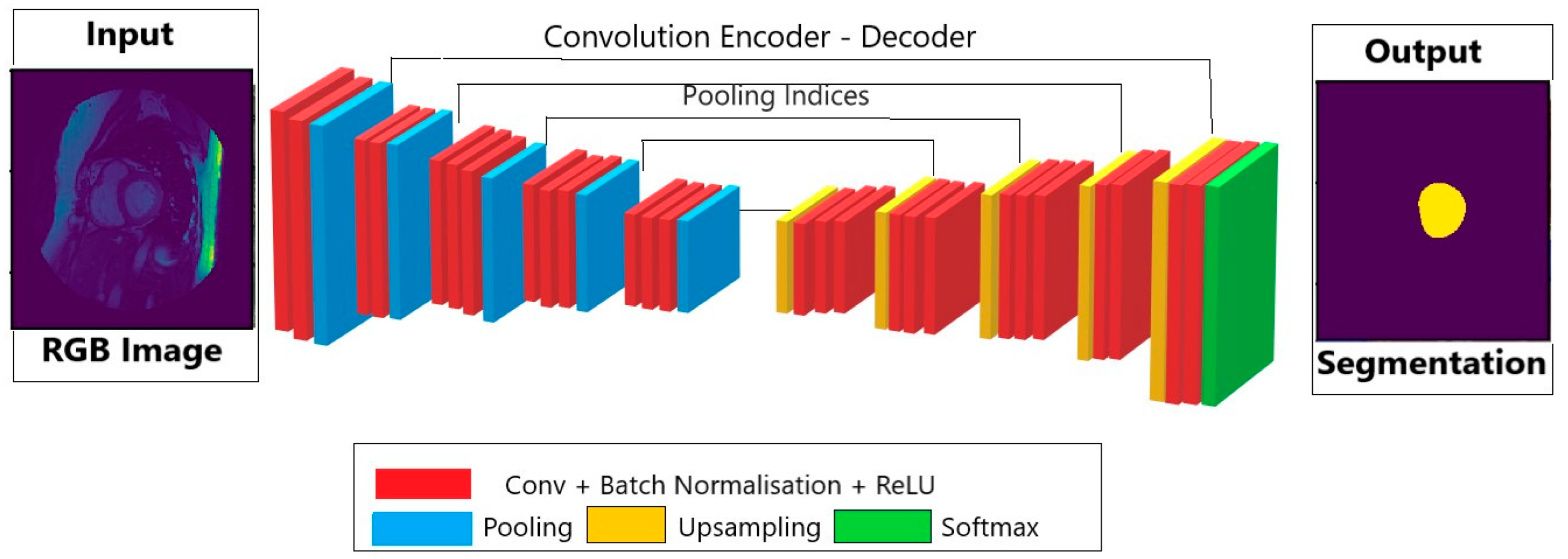
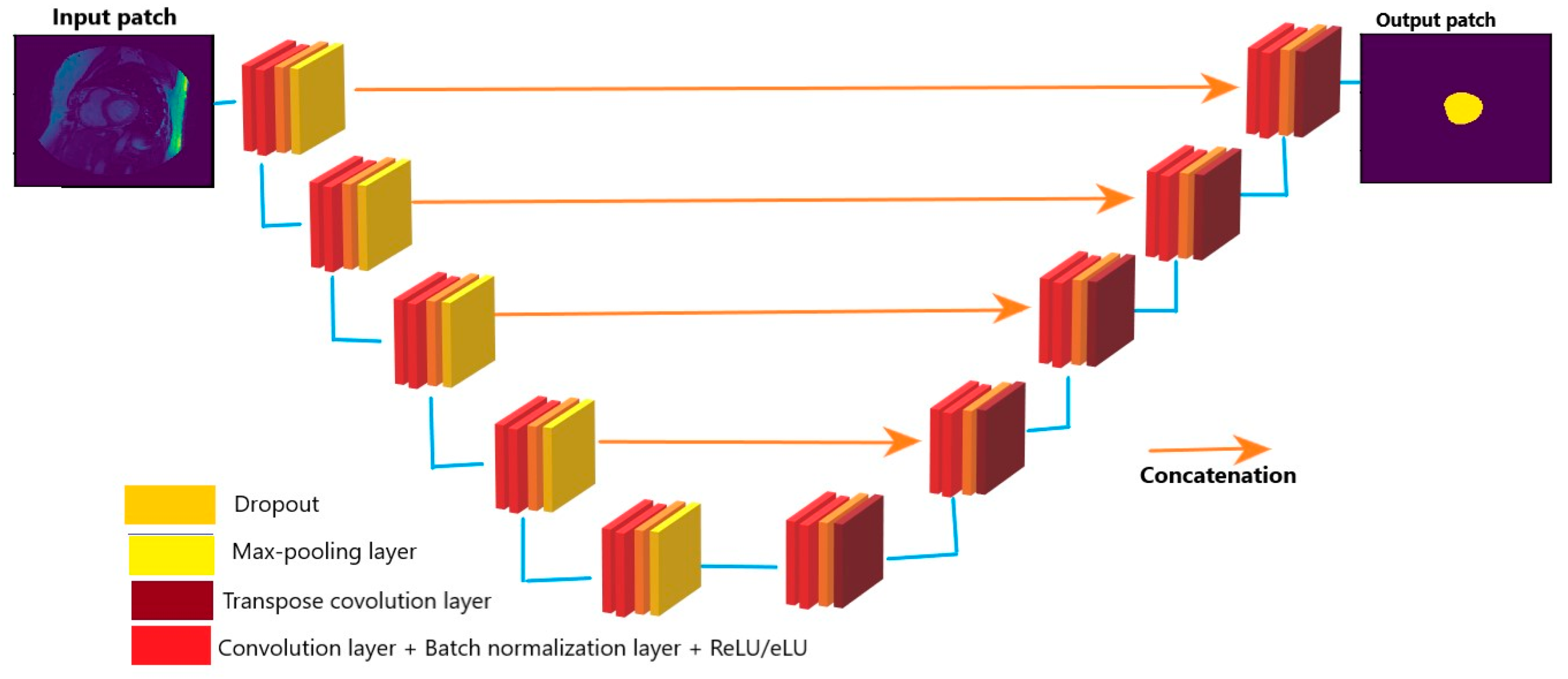
2.1.1. Automatic Segmentation of Cardiac MRI

To perform the segmentation of LV myocardial boundaries, such as endocardium and epicardium in 2D cardiac MR images, the U-Net model with various hyperparameters is evaluated to investigate the generalization capability of the model. The hyperparameters selected for the investigation are:

• Batch size;
• Batch normalization;
• Activation function;
• Loss function; and
• Dropout.

The standard architecture of the U-Net [14] is used. The number of blocks in the contracting and expanding path are optimized as per the hardware. Figure 4 shows the proposed U-Net architecture.

In contrast to the base U-Net architecture, all convolution operations are followed by batch normalization. Unlike only the Relu [27] activation function in the standard U-Net architecture, the Elu [28] activation is also used. A 10% dropout is employed after two convolution operations, i.e., 10% of hidden units are randomly switched off, which makes the deterministic model Bayesian. The architecture contains a contracting and an expansion path, each with five successive blocks. Each block performs the following operations:

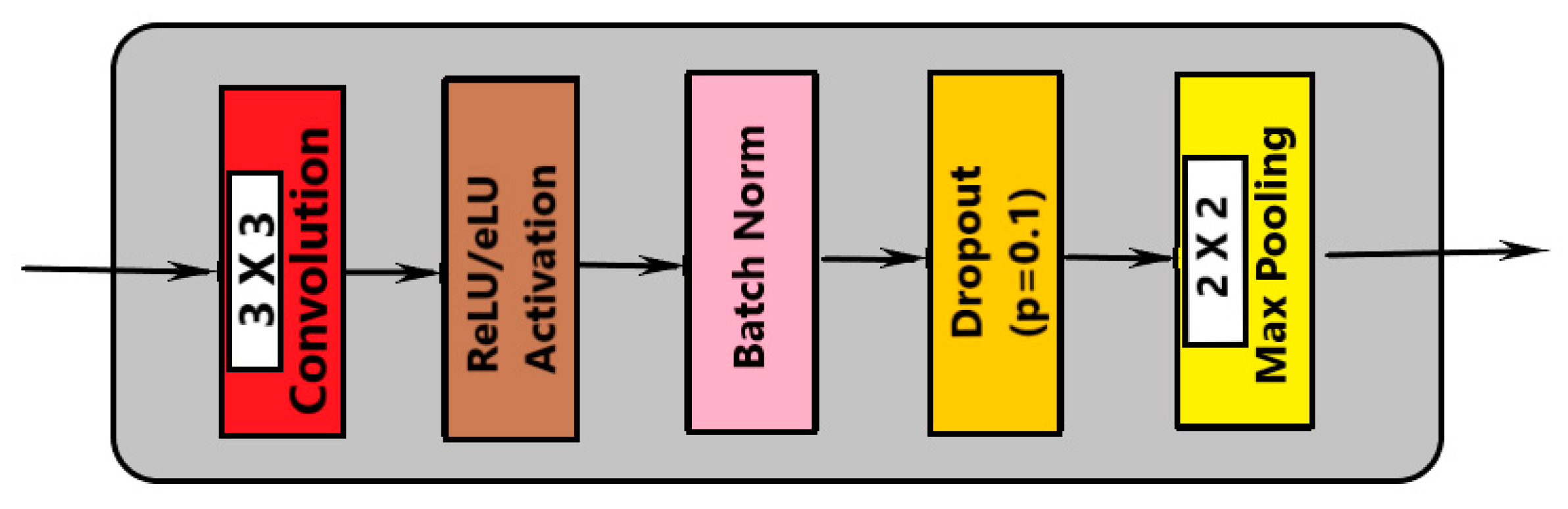
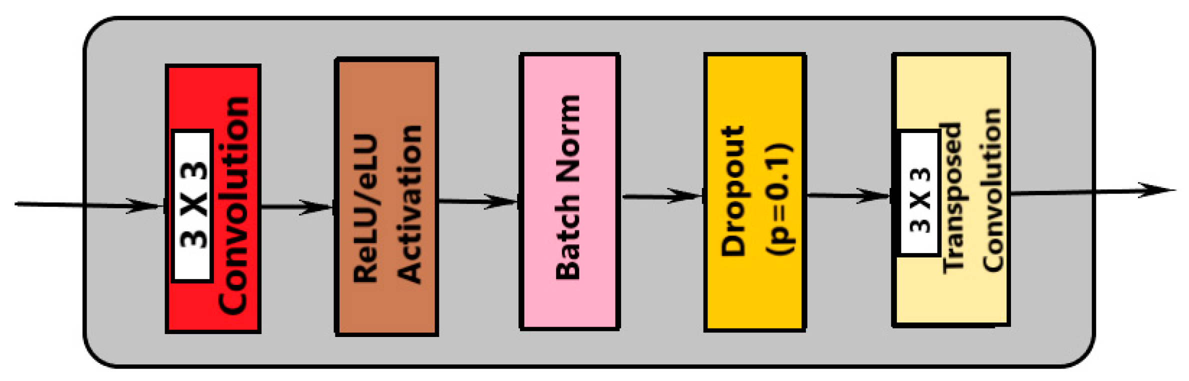
• Convolution with 3 × 3 kernel size;
• Batch normalization;
• Convolution with 3 × 3 kernel size;
• Batch normalization;
• Dropout;
• Max pooling (in contraction and transpose convolution in expansion).

Operations performed in each layer of the contraction and expansion paths are shown in Figure 5 and Figure 6, respectively. It can be seen from the figures that five types of operations are performed at each layer. The only difference between the block in the contraction and expansion path is in the last layer. The pooling layer in the expansion path is replaced by the transposed convolutional layer.

The convolution kernels are initialized with the kernel initializer called He Normal. Generally, the size of the images in each dimension decreases by a factor of k-1 after each convolution operation, where k is the kernel size. However, we retain the size of the image throughout the convolution operations. The size retention is achieved using zero padding. The max-pooling operation is employed at the end of the convolution operation in the contraction path using a 2 × 2 convolutional kernel and stride 2, which down-samples the input array by a factor of 2. However, the transpose convolution operation is employed at the end of the convolution operation in the expansion path, which up-samples the input array by a factor of 2. For instance, if the size of the input image is 256 × 256 and kernel size is 3 × 3, then after convolution the size will be (256 − 3 + 1) × (256 − 3 + 1), i.e., 254 × 254 and 127 × 127 after max-pooling with a 2 × 2 convolutional kernel. Similarly, if the input array size is 127 × 127, then after transpose convolution, the size becomes 254 × 254. After every down-sampling, the number of feature channels increases by a factor of 2. While after each up-sampling, the number of feature channels decreases by a factor of 2. Initially, we start with 8 feature channels and go up to 128 during contraction, and further decrease to 8 feature channels during expansion. The contracting path captures the context, and the expansion path enables the precise location. Therefore, starting with a smaller number of feature channels may decrease the chance of overfitting and improve the context capturing capabilities of the network.

2.1.2. Number of Convolution Layers

Model performance was evaluated with U-Net with different sizes. The results in

Table 3. Model performance with convolutional layers.

Convolution Layers	Training Weights	Training Time (100 Epochs, 2 GPUs)	Performance (Dice Coefficient)
18	1.9 M	4 h	92–93%
23	31 M	6 h	94–96%
28	32 M	7.5 h	94–96%

shows that U-Net with 23 convolution layers is more optimal with training time and accuracy. Adding more layers did not improve the accuracy of the model.

2.1.3. Number of Filters

Model performance was evaluated with 16, 32, and 64 filters at the first convolution layer on the decoder path. The number of filters is doubled at every subsequent convolution layer (64- > 128- > 256- > 512- > 1024). The model with 64 filters at the first convolution layer showed the best performance.

2.1.4. Batch Normalization

We experimented with adding a batch normalization layer between every convolutional layer and activation layer in both the encoding and decoding paths. The default parameters for the batch normalization layer, as implemented in Keras, were used. We did not see any significant changes in the dice coefficient, accuracy, precision, recall, or F1-score. No significant changes in training time were observed either.

2.1.5. Dropout Layers

We also experimented with adding dropout layers before each up-sampling layer in the encoding path. Dropout levels of 20% and 50% were tested. Although our tests indicated that adding dropout layer did not improve the performance of the model, we did include dropout layers in our final model since many of the solutions we studied suggested performance improvement with them. In our final model, a dropout layer of 50% was added after each convolution layer in the encoding path for a total of four dropout layers.

2.1.6. Loss Functions

In medical imaging, segmenting the region accurately is always desirable. Additionally, the segmentation accuracy depends on the quality of training. Deep learning algorithms use gradient-based optimization to enhance the quality of training. Training is an optimization problem that optimizes weights based on objective value. Therefore, the quality of training largely depends on the loss functions. In this research, we investigated the impact of different loss functions on segmentation. Generally, the loss functions are categorized into four broad categories [29]. These are shown in

Table 4. Distribution of loss functions based on its types.

Type	Loss Function
Distribution-based Loss	Binary Cross-Entropy Weighted Cross-Entropy Balanced Cross-Entropy Focal Loss Distance map derived loss penalty term
Region-based Loss	Dice Loss Sensitivity-Specificity Loss Tversky Loss Focal Tversky Loss Log-Cosh Dice Loss
Boundary-based Loss	Hausdorff Distance loss Shape aware loss
Compounded Loss	Combo Loss Exponential Logarithmic Loss

.

Region-based loss functions aim to minimize the mismatch or maximize the overlap regions between ground truth and predicted segmentation. Therefore, we considered region-based loss functions because we were trying to maximize the overlap regions, since binary cross-entropy is the default loss function in deep learning models. For this reason, we considered that too. The detailed descriptions of loss functions can be found in [29].

2.1.7. Optimization

We trained the network using the proposed U-Net architecture with Relu- and Elu- activation functions. We investigated the performance of segmentation using different loss functions. So, there are 10 combinations overall to be investigated, as shown in

Table 5. Total combinations investigated.

Activation Function	Loss Function	Activation Function	Loss Function
Relu	Binary Cross-Entropy	Elu	Binary Cross-Entropy
	Dice Loss		Dice Loss
	Log-Cosh Dice Loss		Log-Cosh Dice Loss
	Tversky Loss		Tversky Loss
	Focal Tversky Loss		Focal Tversky Loss

. All the models were trained on an 8 GB NVIDIA GeForce RTX 2070 GPU card, 32 GB RAM, and Xeon E5 Processor. An ADAM [30] optimizer was used to minimize the loss function to obtain a better accuracy.

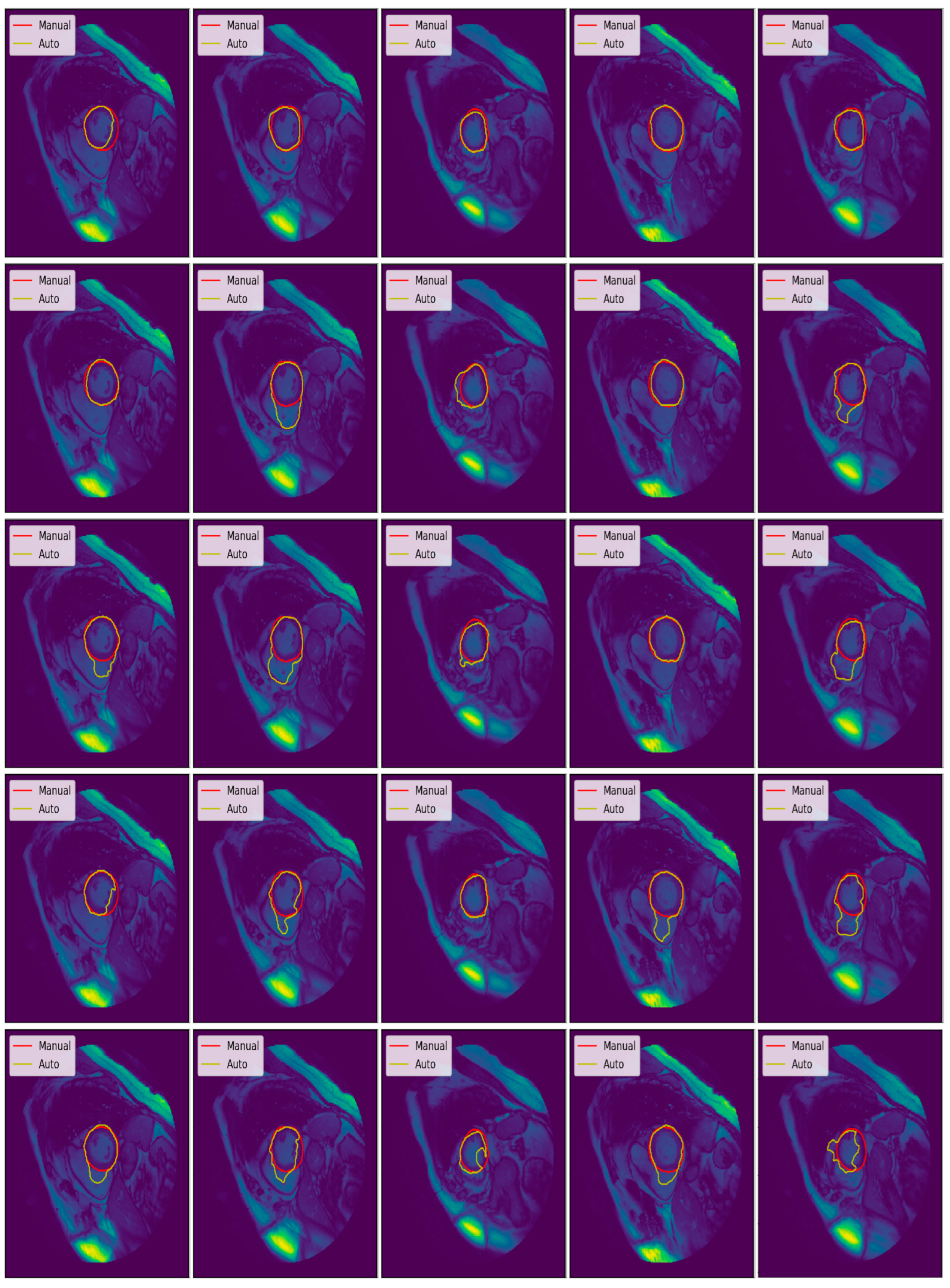
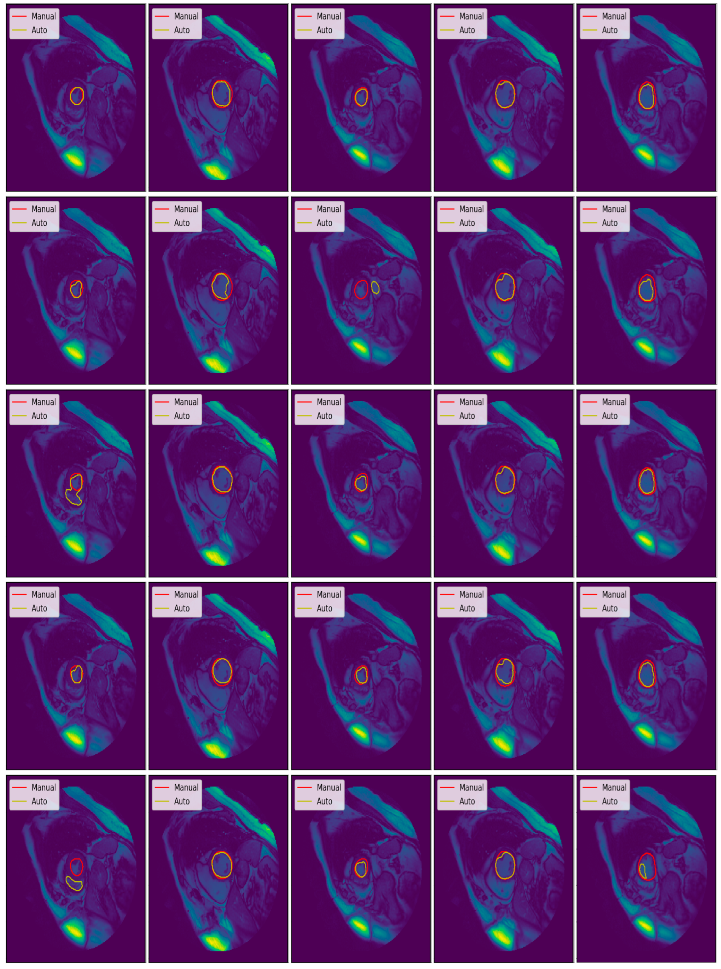
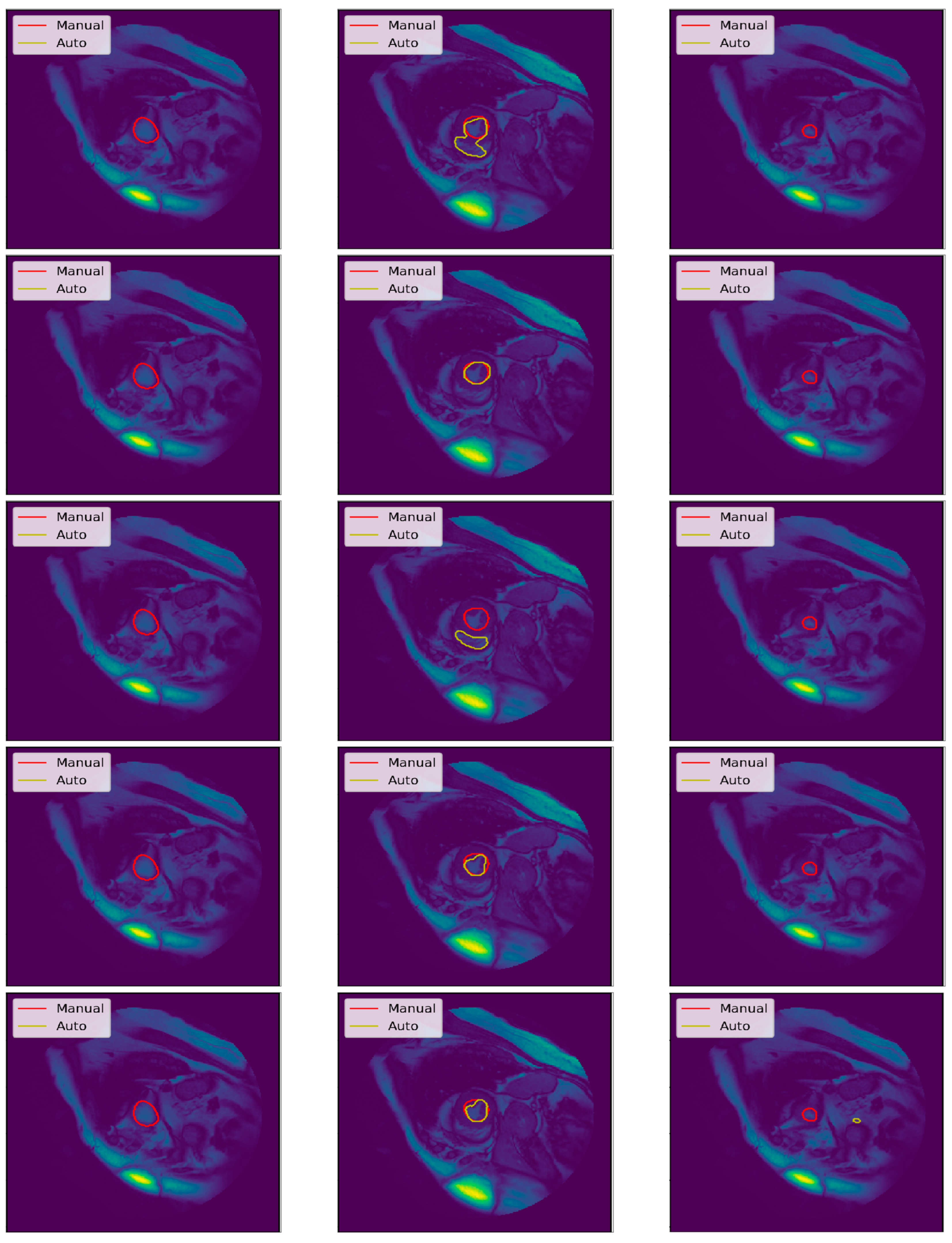
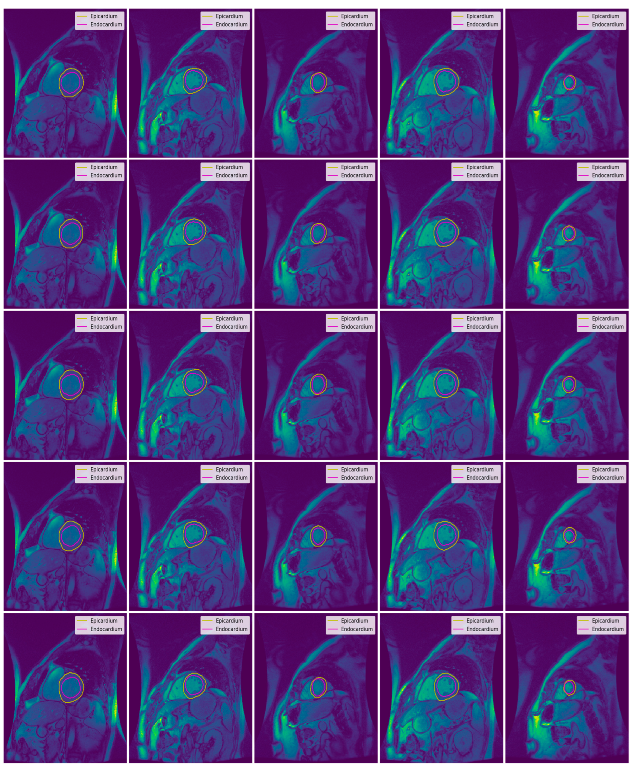
2.2. Performance Evaluation

2.2.1. Segmented Accuracy Assessment Metrics

The performance of the models was evaluated in terms of average perpendicular distance (APD), dice metric, and percentage of good contours. However, all the clinical factors, such as average ESV, EDV, and EF based on all modes, were also computed. The evaluation parameters are defined below.

• Average perpendicular distance measures the distance between manual and auto contours, averaged over all contour points [31]. It was used to measure the closeness of the segmented boundaries; the smaller the value, the closer is the boundary. The value of APD measures in millimeters with the help of pixel spacing provided in the DICOM field named PixelSpacing.
• The dice metric was used to measure the overlapping or similarity between manual and auto contours. Its value lies between 0 to 1, where 0 means no overlap and 1 means perfect overlapping. The dice metric between auto and manual contours can be defined as:

  $$DM\left(Auto,Manual\right)=2\frac{Auto \cap Manual}{Auto + Manual}$$
• The percentage of good contours is evaluated in terms of APD. It is basically the fraction of contours out of total contours. The fraction of contours is selected if APD < 5 mm.

2.2.2. Clinical Metrics

Clinically relevant factors, such as ESV, EDV, and EF, are also calculated. EF can be calculated as:

$$EF=\frac{SV}{EDV}\times 100\%$$

where $SV$ is stroke volume and can be calculated as $SV=EDV-ESV$.

Furthermore, the clinical parameters are analyzed using regression and the Bland–Altman plots.

3. Results and Discussion

In this research, 45 cases were tested. Initially, batch size and dropout were finetuned to carry out further processing. We tested three different combinations of the batch size such as 4, 8, and 16, and obtained good accuracy at batch size 4. Additionally, four different combinations of the dropout were considered, i.e., 0.1, 0.15, 0.2, and 0.25, and obtained good accuracy at 0.1 dropout value. Therefore, for the entire experiment, the batch size and dropout were considered as 4 and 0.1, respectively, with active batch normalization. Two activation functions, Elu and Relu, in combination with different loss functions, have also been considered for the experiment. Optimization parameters considered for the research are shown in

Table 6. Hyperparameters and their corresponding values.

Hyperparameters	Value/Name	Hyperparameters	Value/Name
Batch Size	4	Dropout	0.1
Activation Functions	Relu/Elu	Loss Functions	Binary Cross-Entropy Dice Loss Log-Cosh Dice Loss Tversky Loss Focal Tversky Loss
Batch Normalization	True

. Out of 45 patients’ data, 15 were used for training, validation, and testing. Hyperparameters and their corresponding values are shown in Table 6.

3.1. Data Pre-processing

The Baseline Method involved rescaling the images so that each pixel was 1 mm × 1 mm and then cropping the image from the center to either 256 × 256 or 176 × 176.

This method consisted of the following steps:

• Orientation: Orientation shift based on the DICOM InPlanePhaseEncoding metadata, which indicates the axis of phase encoding with respect to the image. A majority of the images were “Row” oriented; thus, if the image was “Col” oriented, it was flipped to be “Row” oriented.
• Rescale: The image is rescaled based on the image’s Pixel Spacing values.
  • Rescale with the first Pixel Spacing value in both the x and y directions;
  • Rescale to 1 mm × 1 mm.
• Crop: The image is cropped from the center to 256 × 256. In this project, 256 × 256 and 176 × 176 were used.
• ROI Location.

In order to identify the left ventricle region of interest (ROI), two approaches were used. The LV ROI crops the MRI image to focus the LV, which is expected to improve the results of the segmentation task in terms of processing and accuracy. By using an ROI image as the input into the U-Net, there is less noise in the image. The LV has four distinct features within the MRI Image that were exploited in order to identify the ROI:

• The heart cavity containing the LV is near the center of the MRI Image;
• The frequency at which the LV moves is unique compared to the frequencies of other heart muscles;
• There is a degree of pixel variance around the LV muscle;
• The LV is circular in shape.

All cardiac MR images are available in the DICOM format, while the boundary coordinates of manual contours are available the in.txt format. All images were resized into 256 × 256 dimensions, and the contour coordinates were converted into the mask of the same dimensions. A sample of the image mask combination is shown in Figure 7.

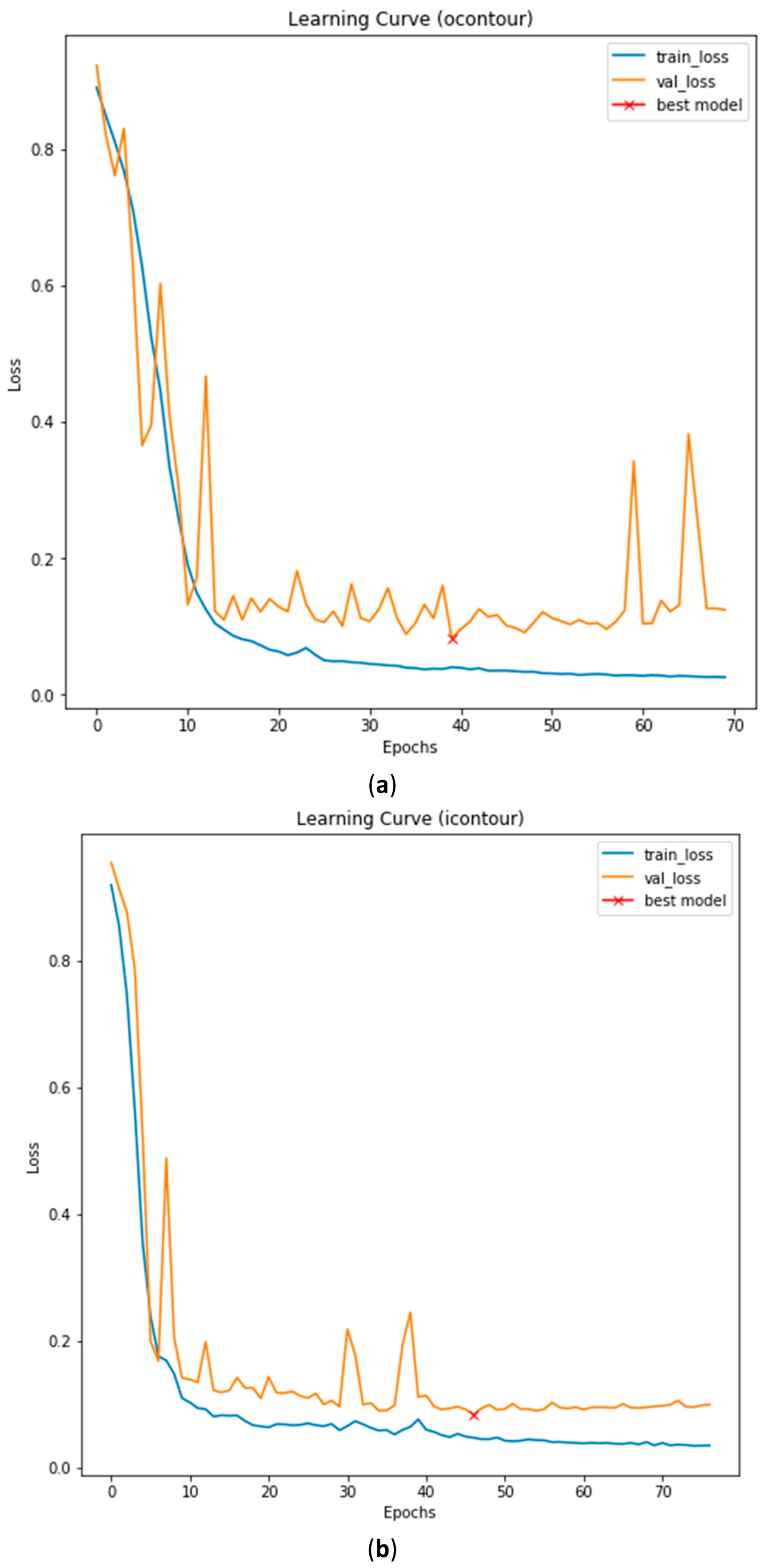
3.2. Data Preparation and Training

Masks of all 45 patients were generated using the approach discussed in the data pre-processing section, then all Dicom images from the training set and their corresponding masks were grouped. The model considers the combination of image and mask and minimizes the loss function to be trained. Therefore, the quality of training depends on how well the minimization of loss function impacts segmentation accuracy. During training, the performance parameters of the model are evaluated based on validation loss. Two different models were developed, one for endocardium detection and another for epicardium detection. The model for endocardium was trained using the endocardium images and masks, while the model for epicardium was trained using the epicardium images and masks. The loss curves of both the models minimizing the dice loss using the elu and relu activation functions are shown in Figure 8a and Figure 8b, respectively. The loss curve minimizing the binary cross-entropy is shown in Figure 9. All the figures contain training loss, validation loss, and the marking of the best model.

To prevent overfitting, we also employed model checkpoints and early stopping conditions. During the training, if there was no further improvement then the trained model was saved for inferencing and training was stopped. We considered 200 epochs for training; however, none of the models used the entire epochs for training. Mostly we obtained a perfectly trained model within 100 epochs, which can also be seen in the learning curves in Figure 9 and Figure 10. Additionally, it can be observed from the above Figures that models with the Elu activation function provide a “good fit”, as the validation error is slightly higher than the training error and became better and better over the time or epochs. However, the difference between validation and training errors was larger with the Relu activation and was not consistent with time. Even after certain epochs, it produced high errors.

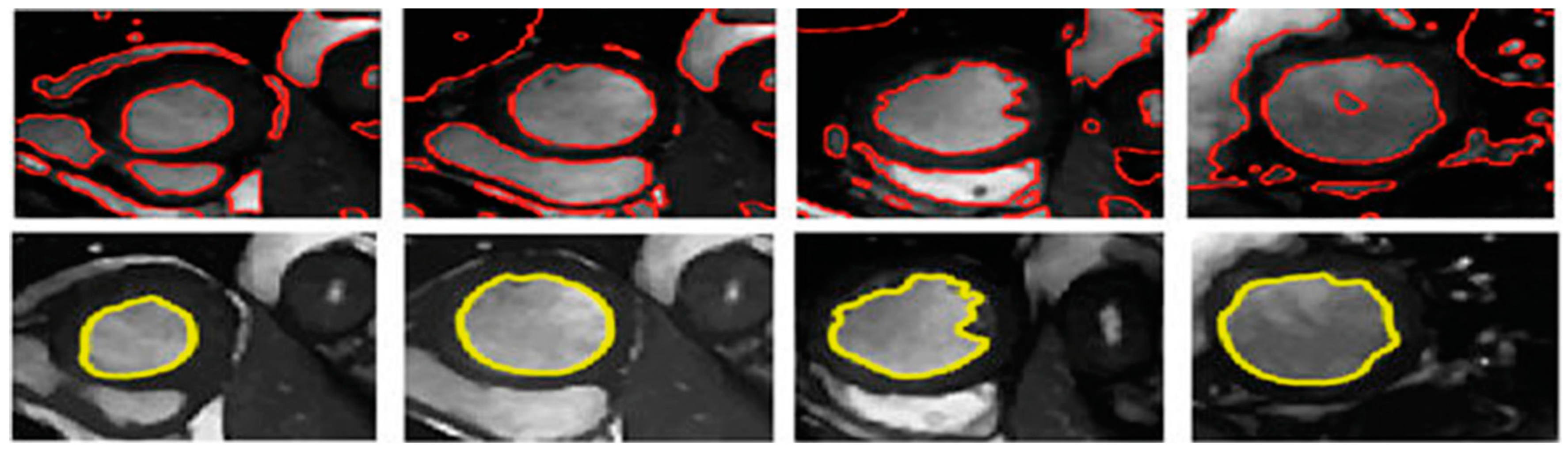
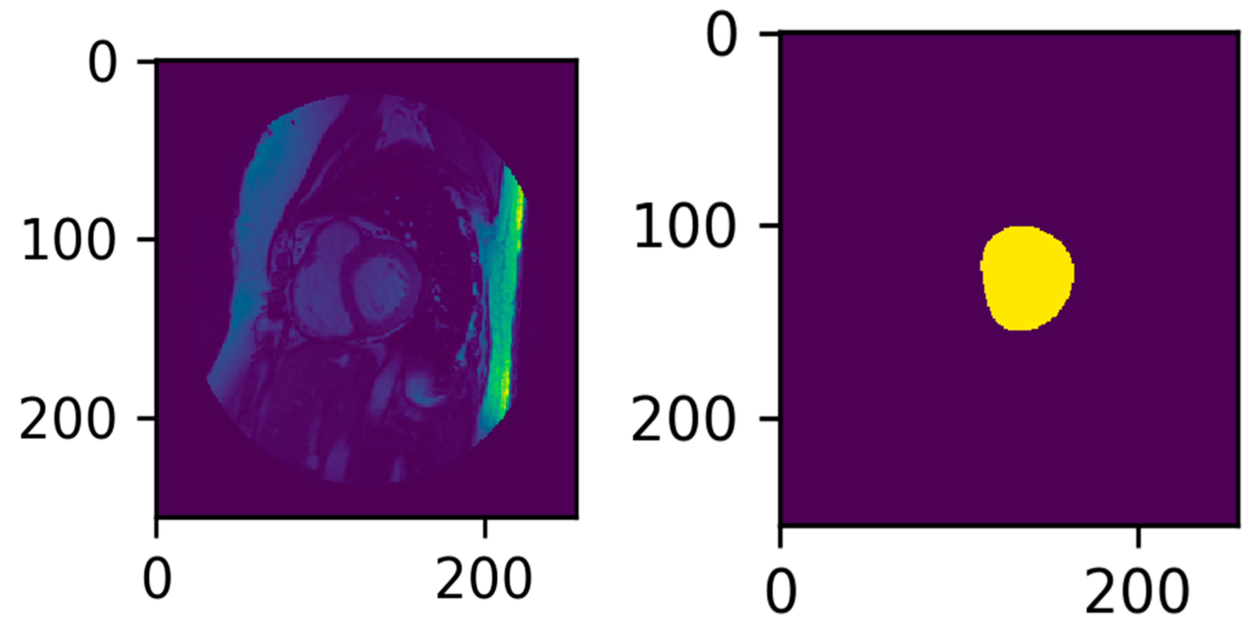
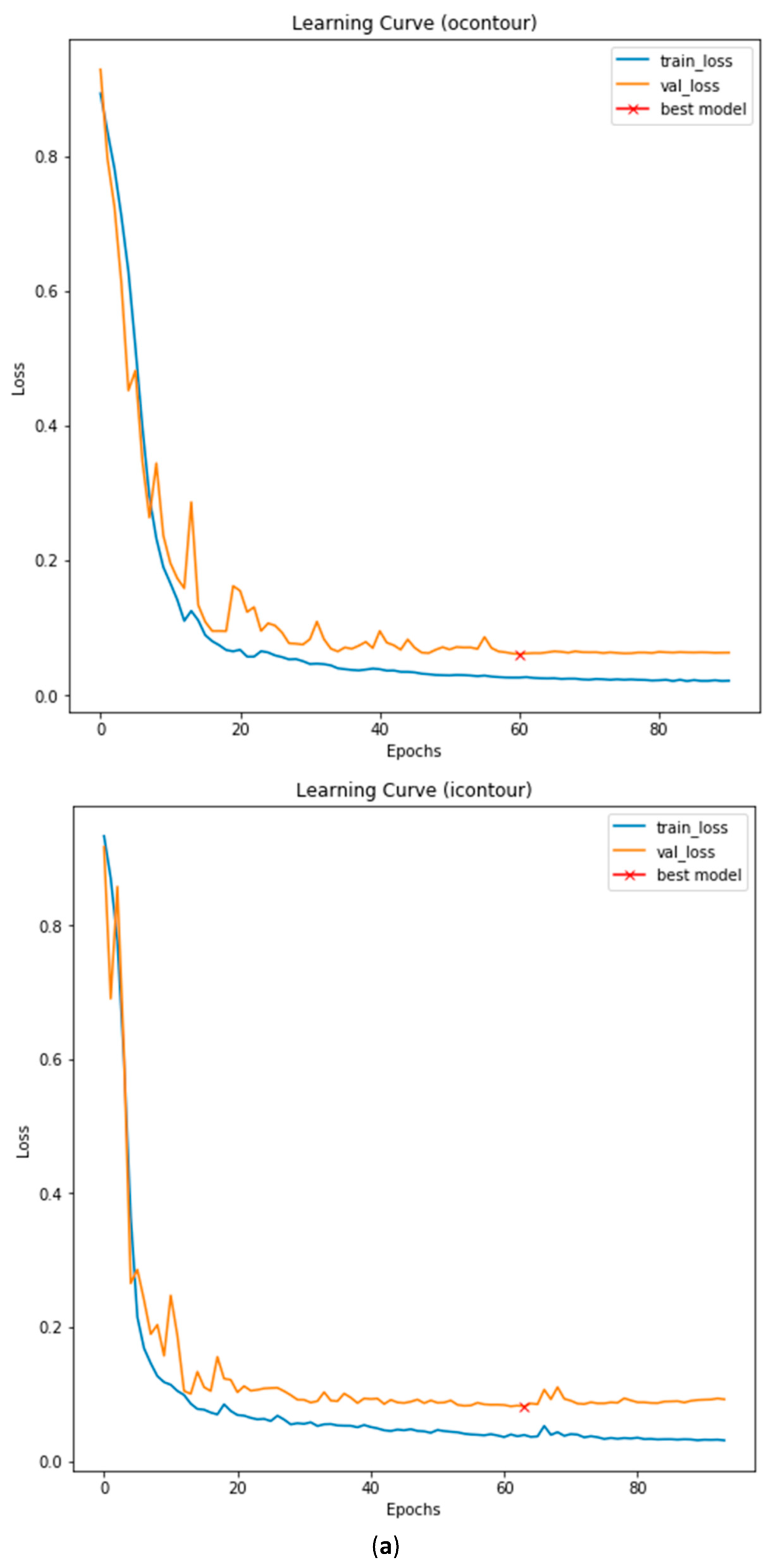
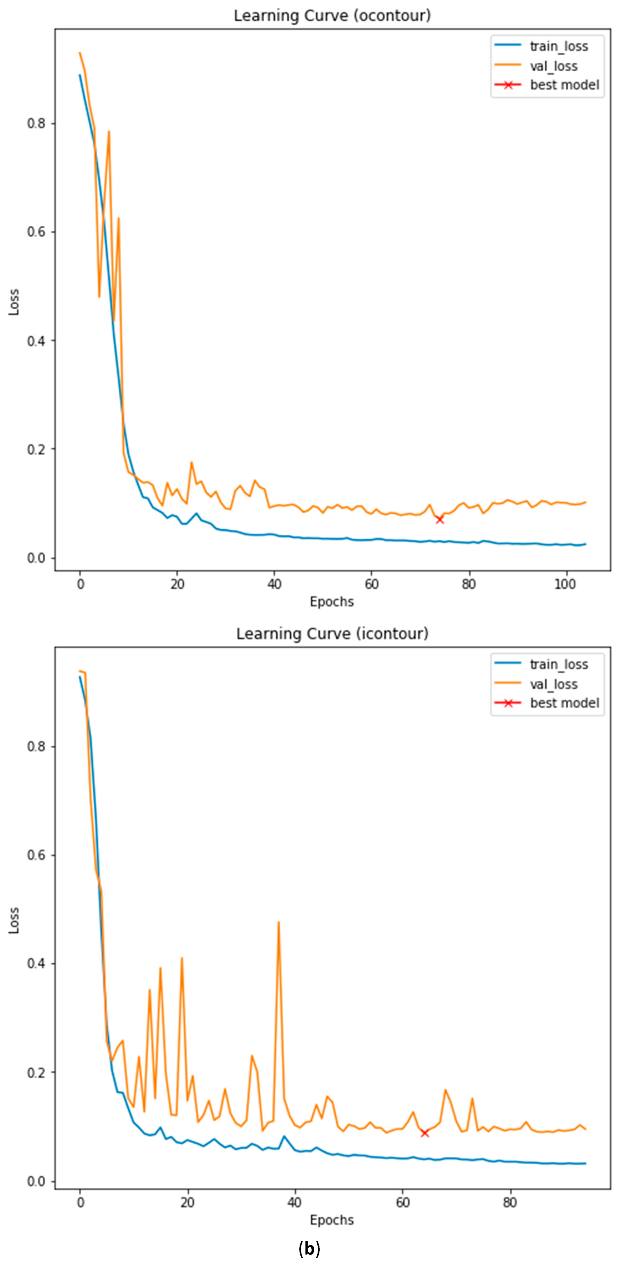
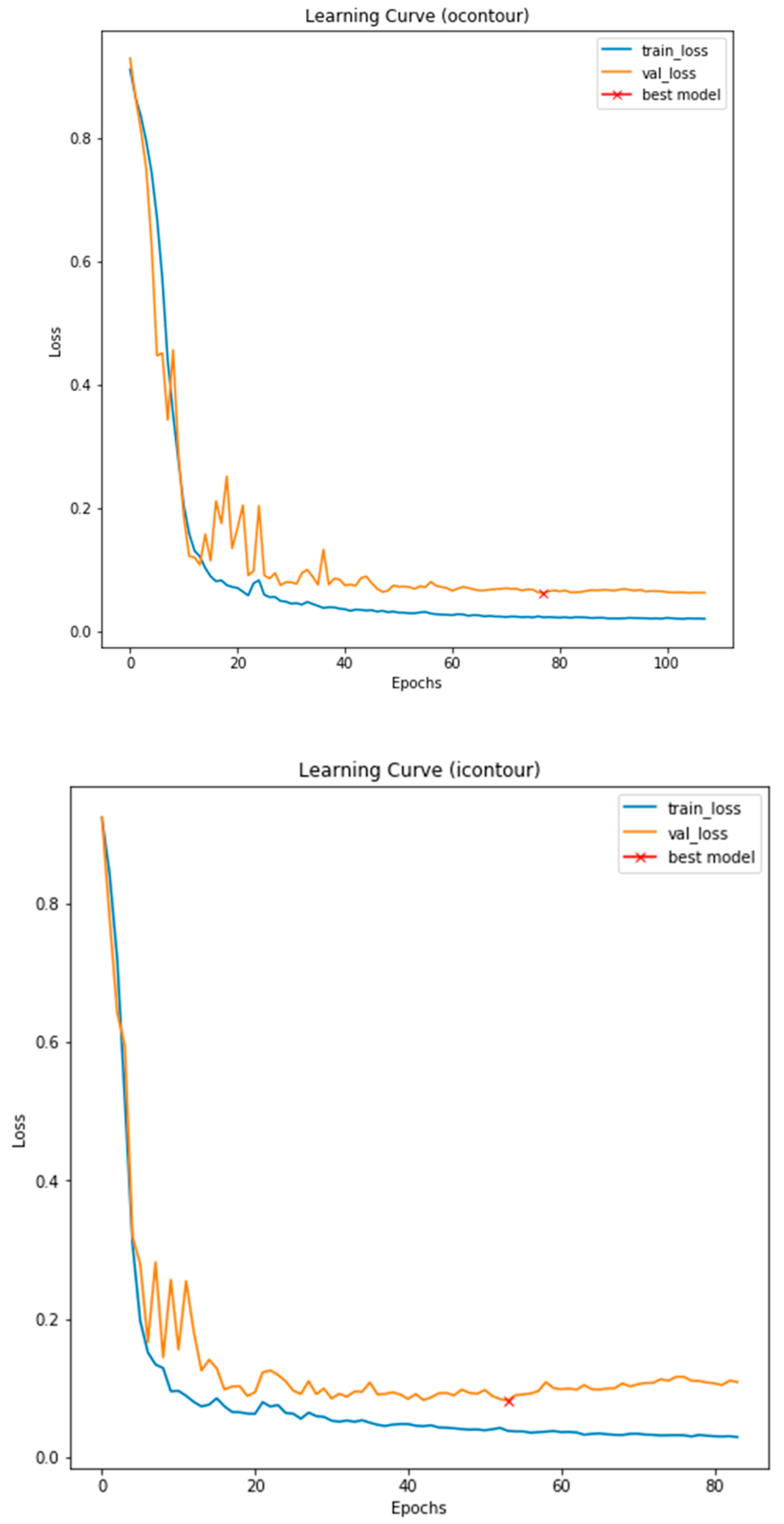
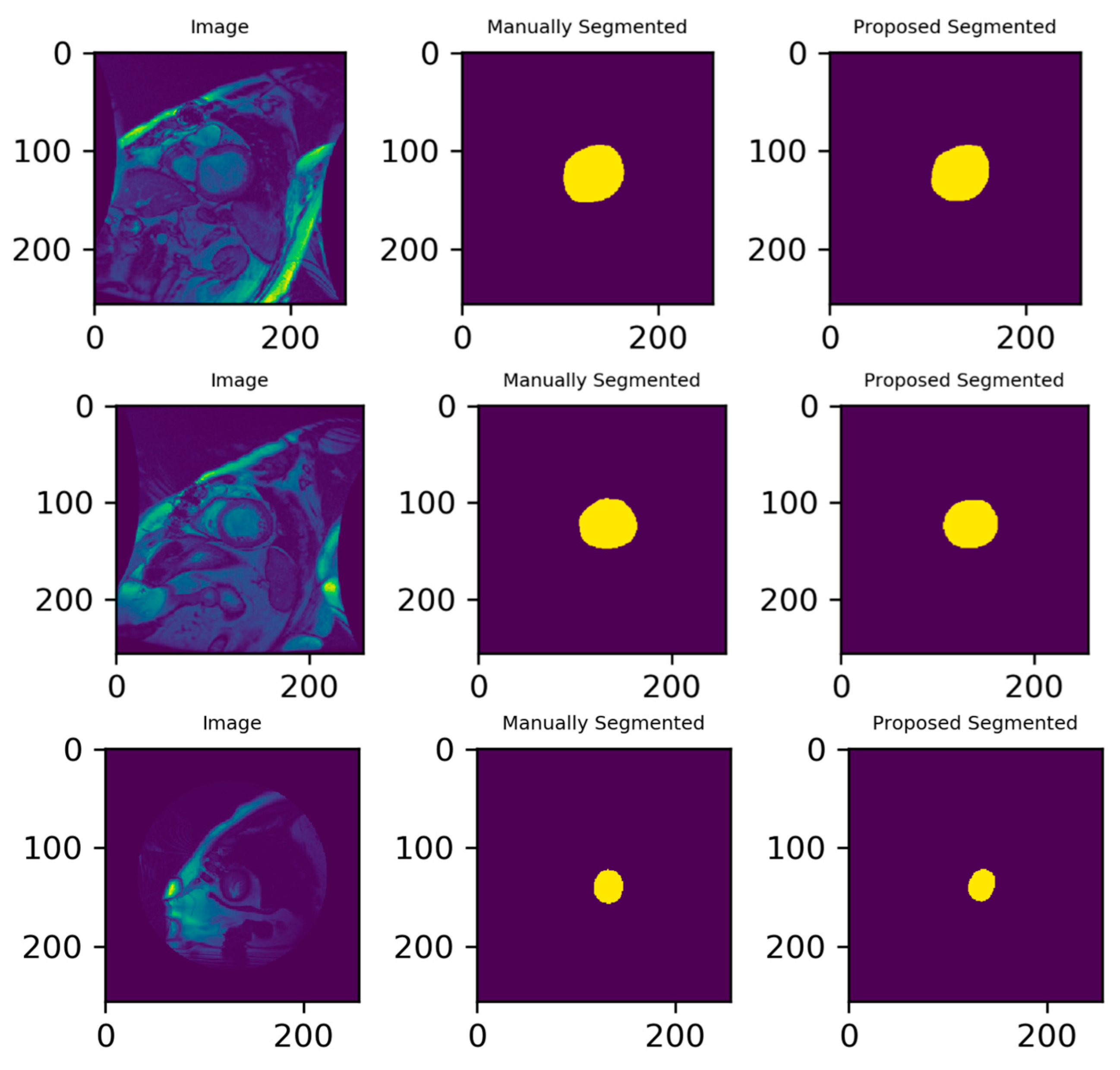
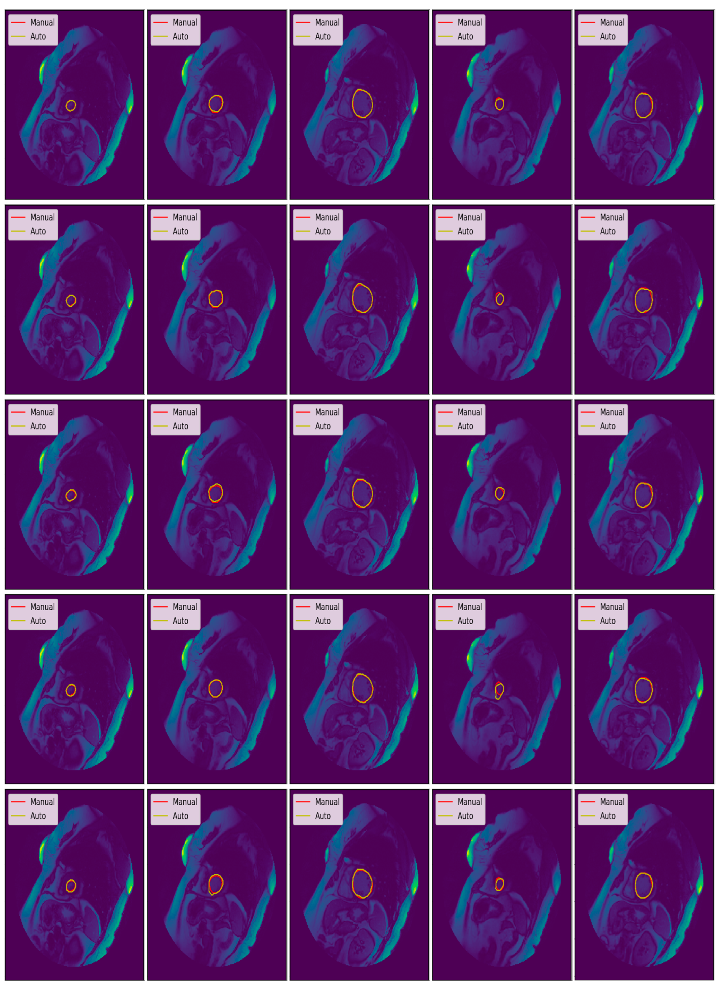
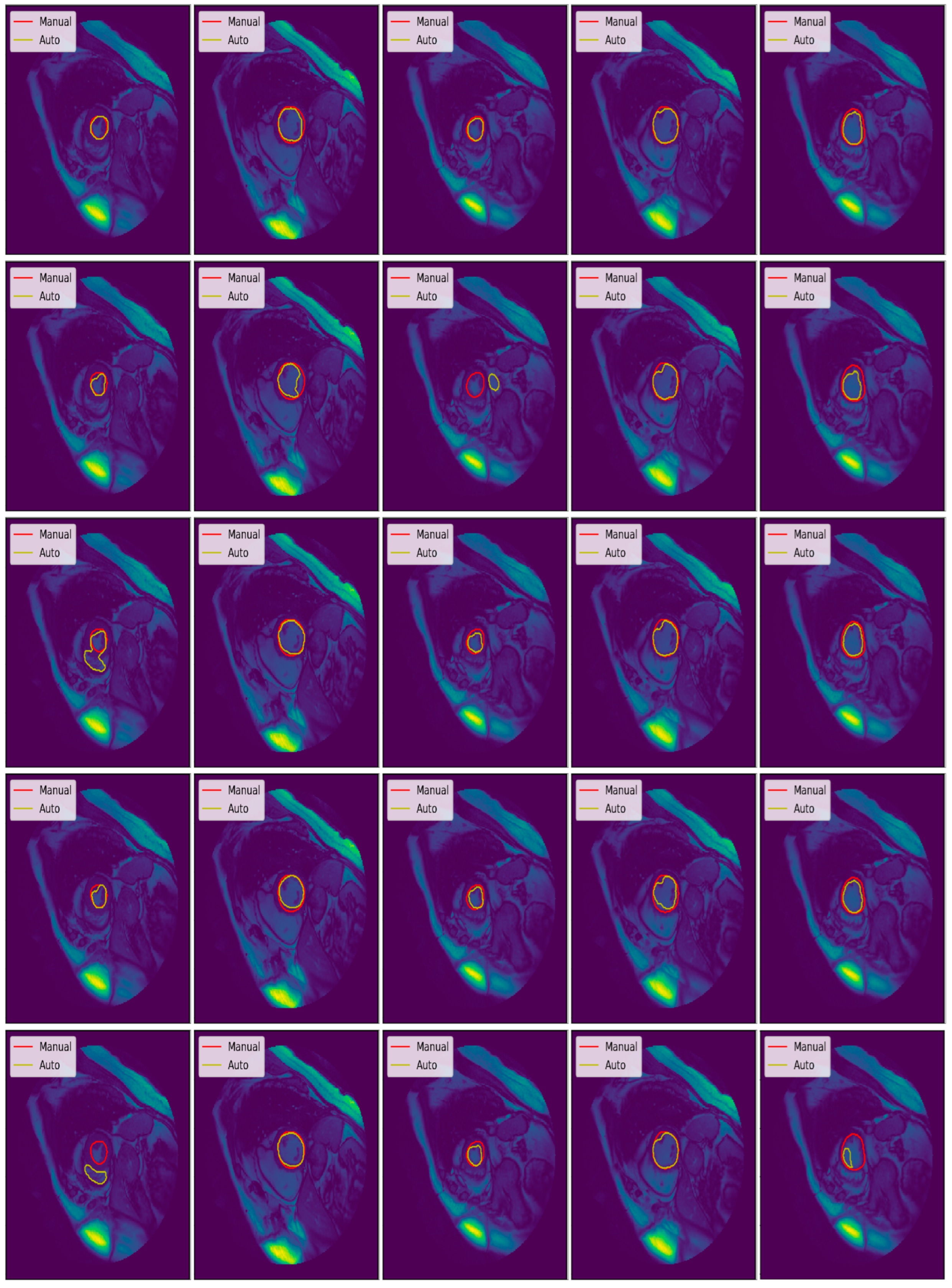
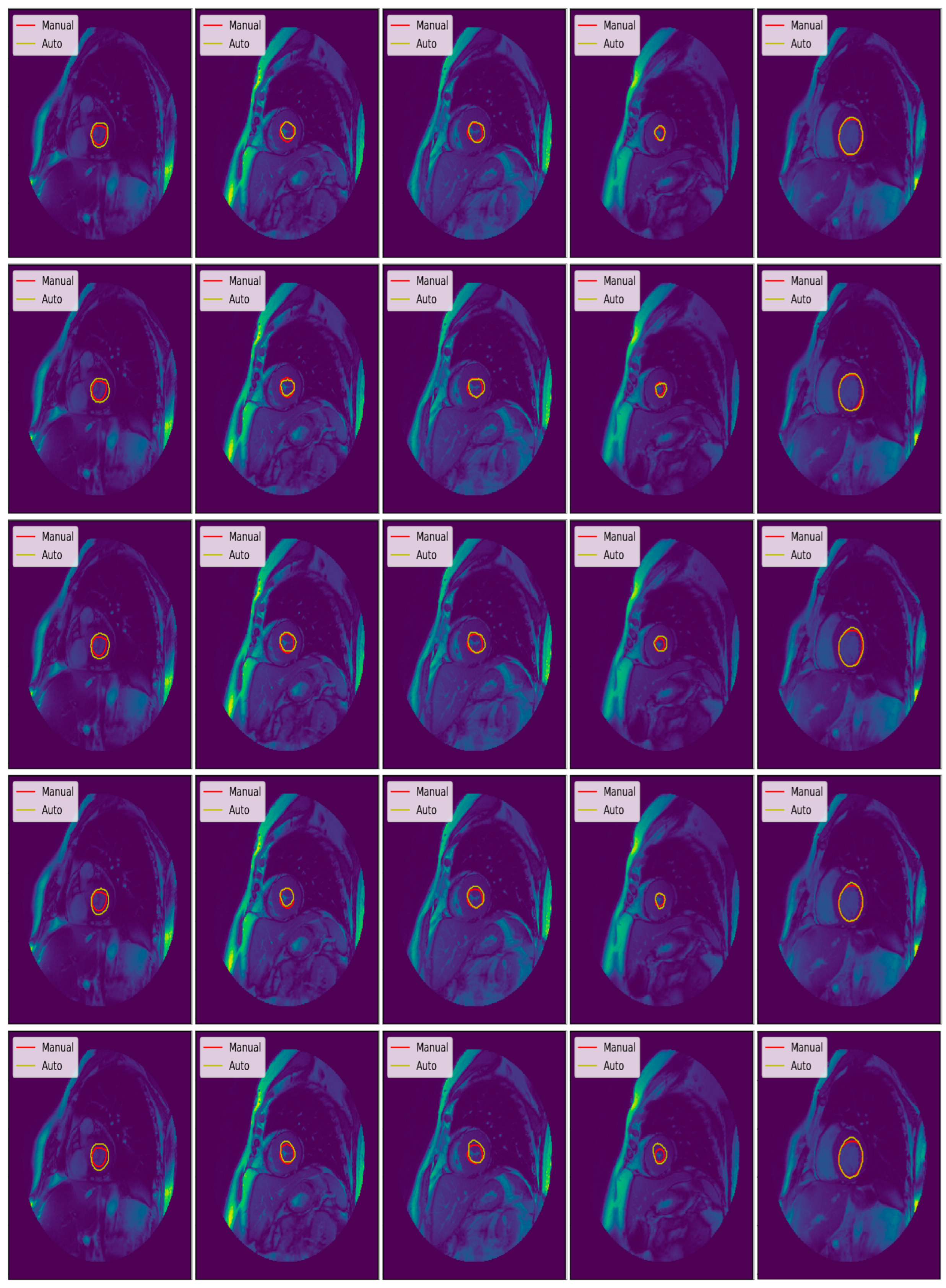
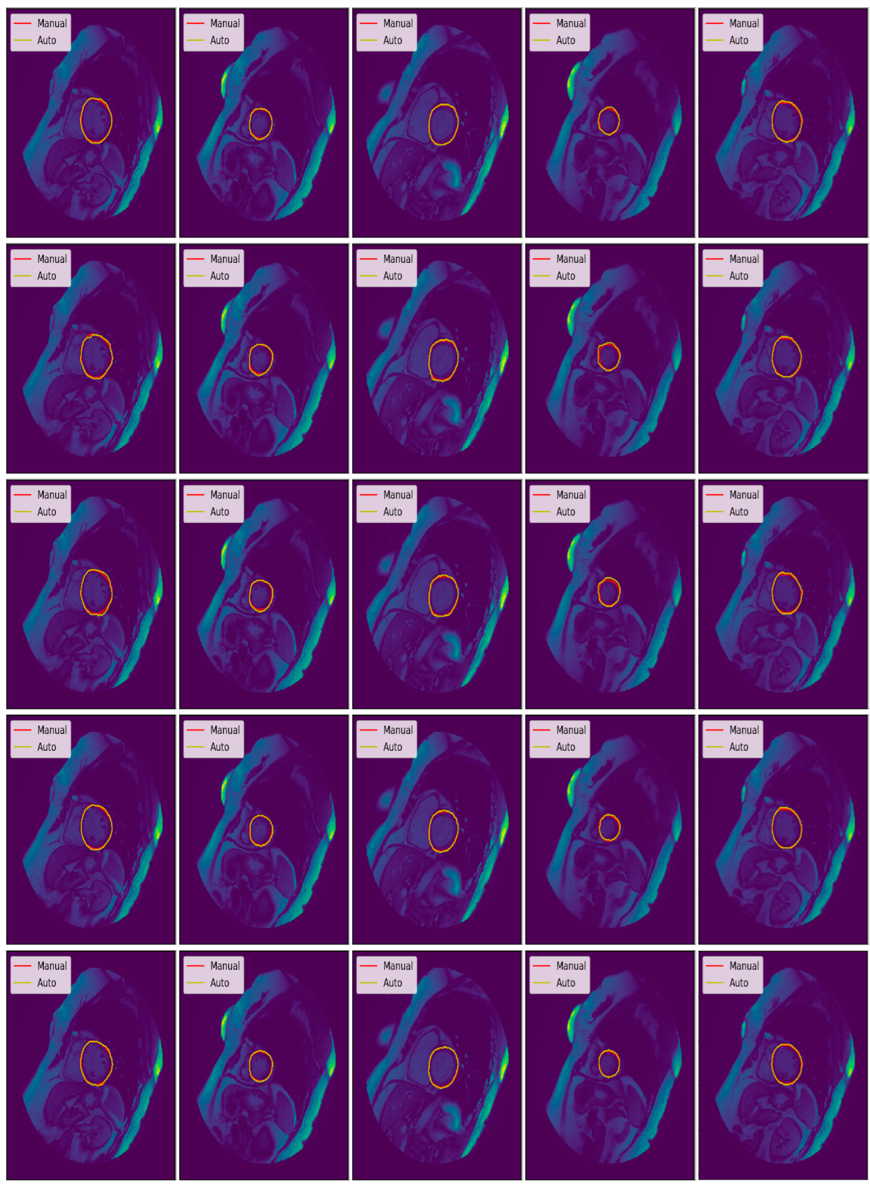
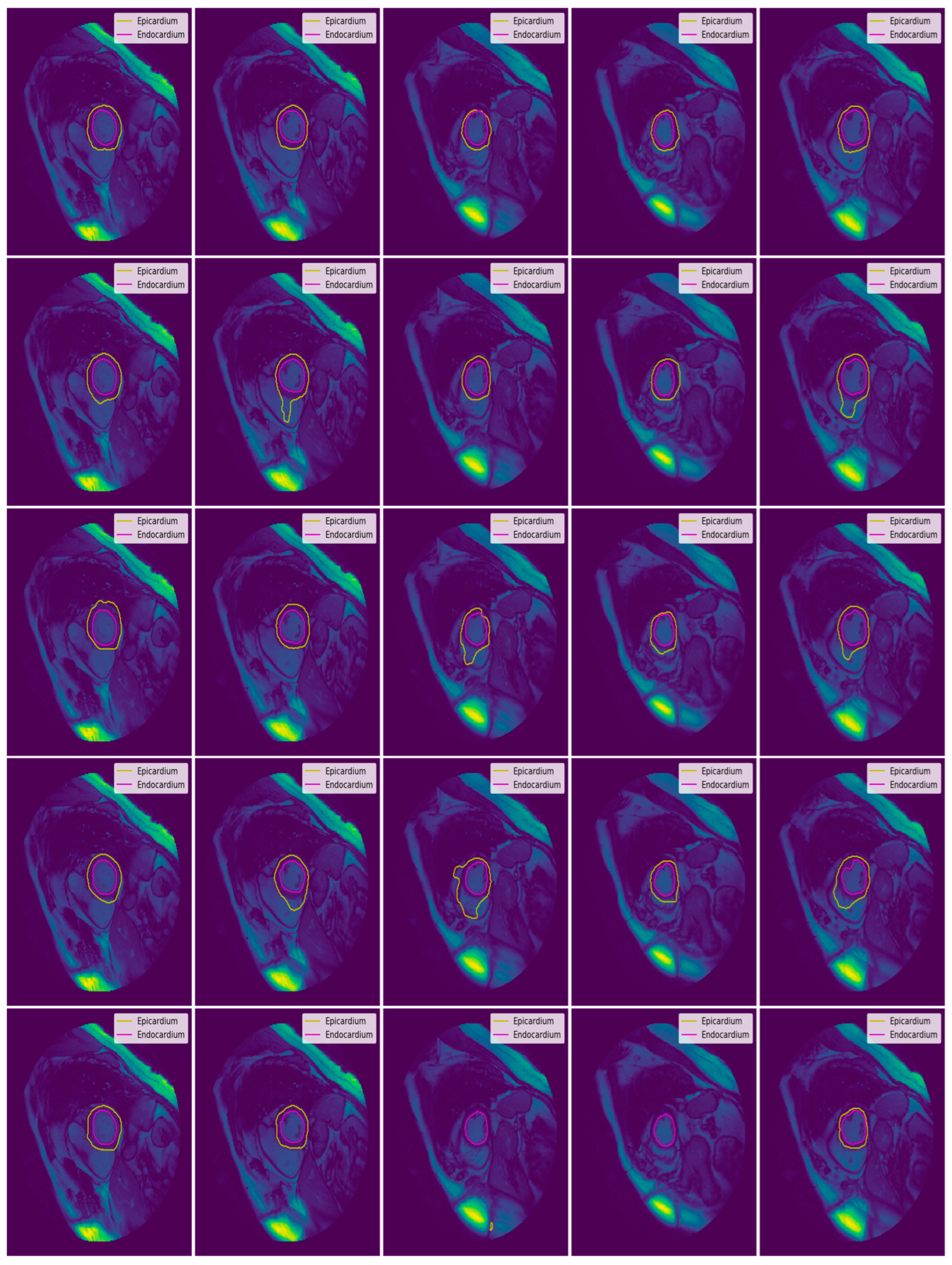
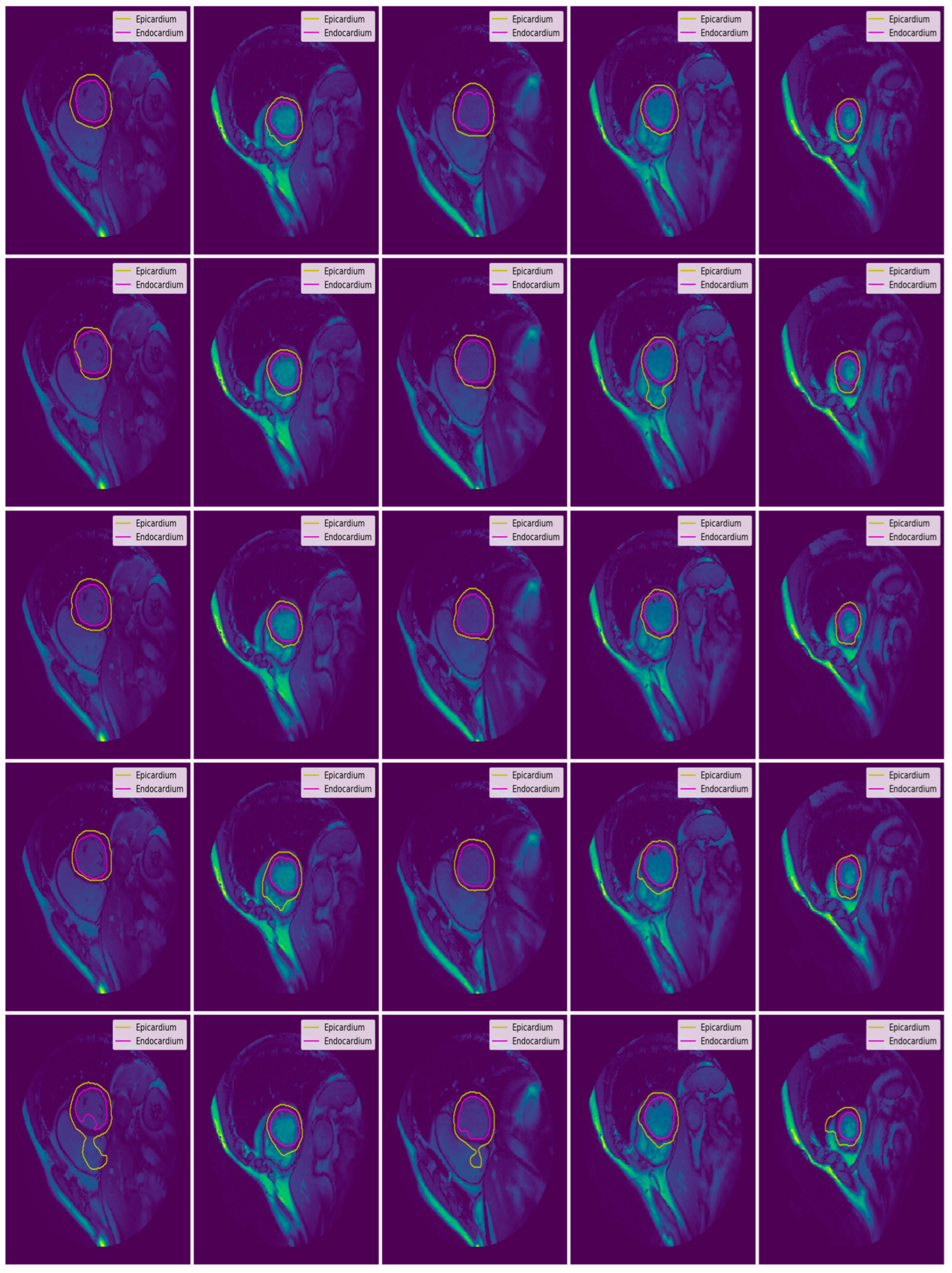
3.3. Illustrated Results

Once the model is trained, then it returns the mask as an output when a cardiac image is given as an input to the model. Automatically segmented outputs from the SC-HF, SC-HF-I, and SC-HYP test samples are shown in Figure 11. Each row contains a cardiac image, manual contour, and automated segmented contour.

Figure 12, Figure 13 and Figure 14 illustrate the manual and automatic segmentation of the endocardium from the training, validation, and testing sets, while the epicardium segmentation is illustrated in Figure 15, Figure 16 and Figure 17. In the figure, manual contours are marked in red, while automatic contours are marked in yellow. Each row corresponds to the model-wise segmentation, where the row-wise order of the models is as follows:

• U-Net with focal Tversky loss;
• U-Net with log-cosh dice loss;
• U-Net with Tversky loss;
• U-Net with dice loss; and
• U-Net with binary cross-entropy loss.

Figure 18 illustrates the missed and wrong classification. Misclassification commonly occurs at the basal and apical slices due to low contrast between the cavity and the surrounding tissues.

Figure 18, Figure 19, Figure 20 and Figure 21 illustrates the automatic segmentation of epicardium and endocardium from the training, validation, and testing sets for the SC-N category. The epicardium boundary is marked with yellow color, while the endocardium boundary is marked with magenta color.

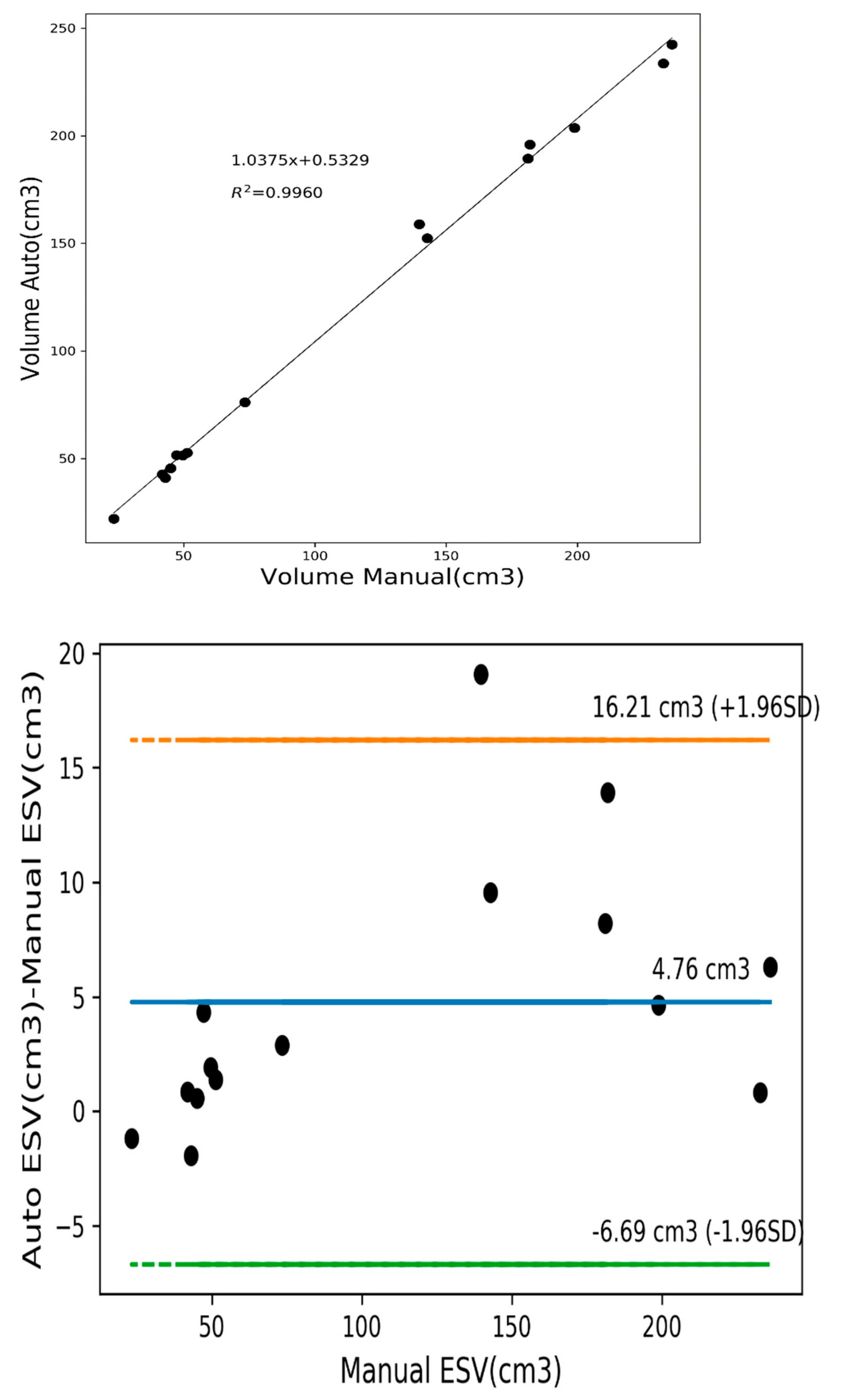
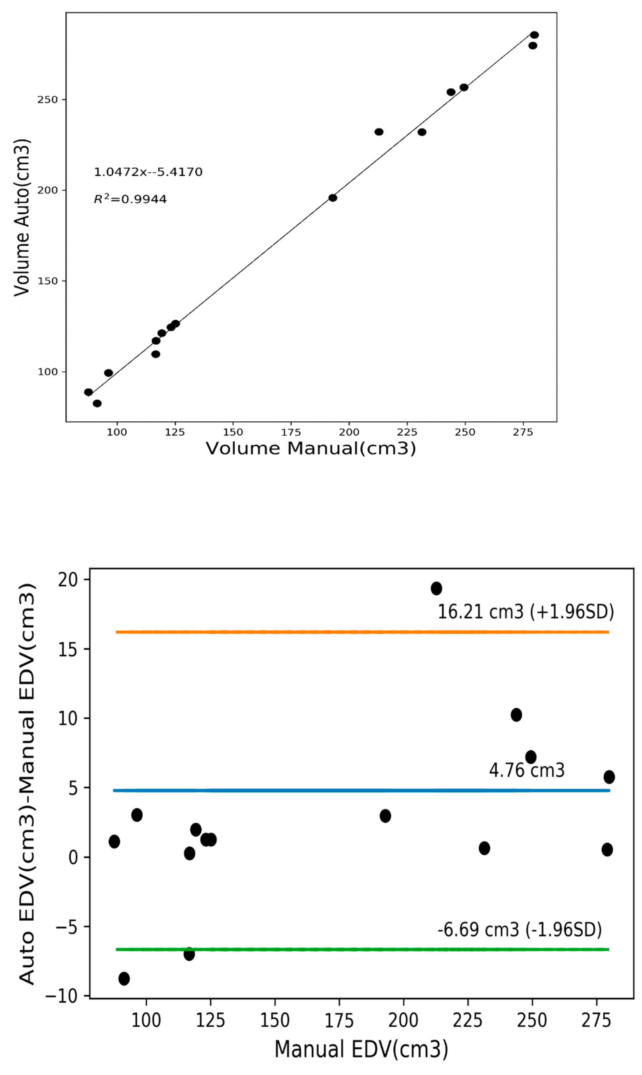
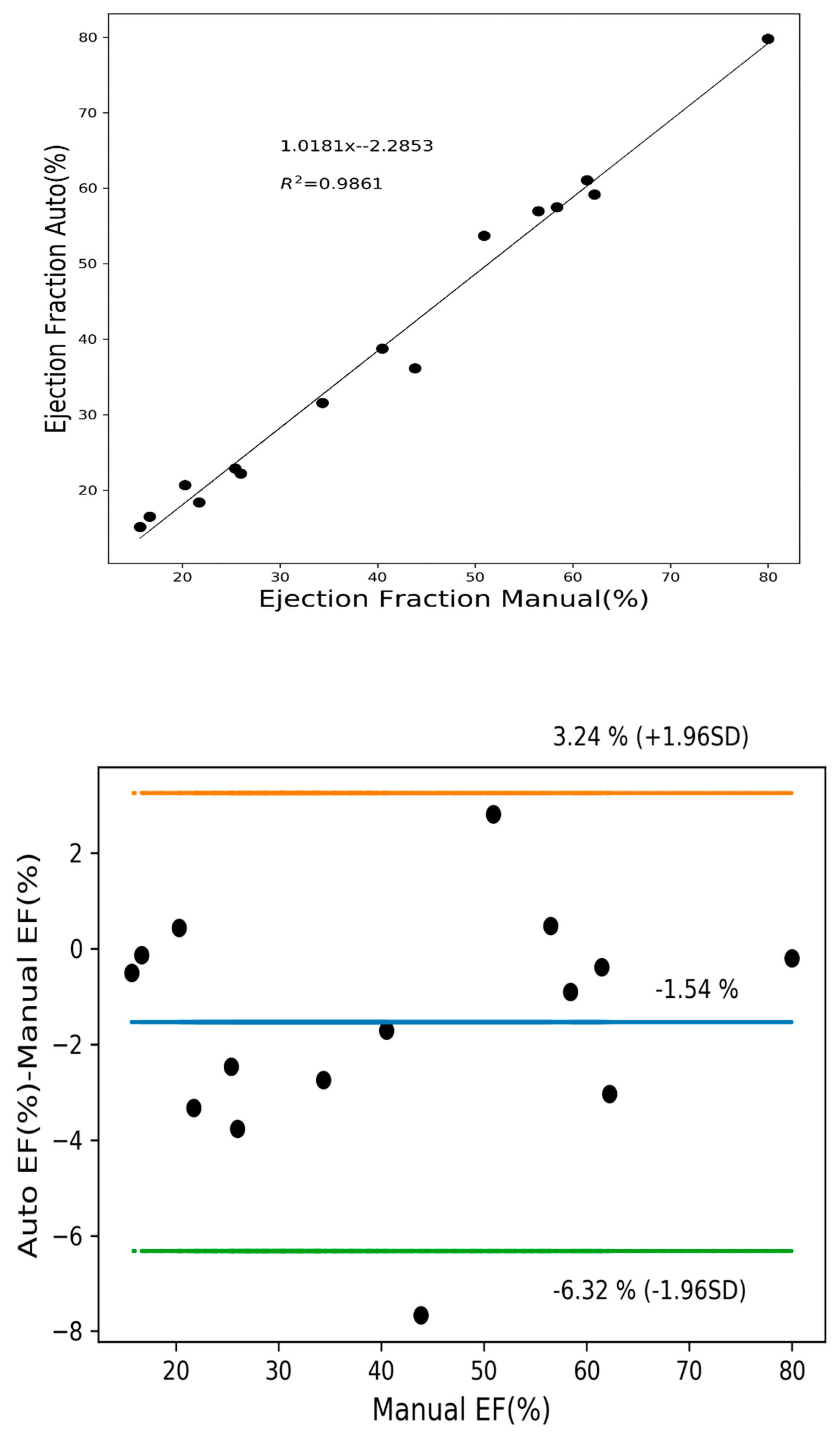
3.4. Quantitative Analysis

The overall statistics of the automated segmentation results are shown in

Table 7. Performance evaluation parameters for dice loss and Elu activation.

Patient Group	Cases	Average Contour Detection (%)		Average Good Contour Detection (%)		Average Perpendicular Distance (mm)		Dice Metrics
		Endo	Epi	Endo	Epi	Endo	Epi	Endo	Epi
N	9	100	100	96.89	95.63	1.65	2.04	0.91	0.93
HYP	12	100	100	95.70	89.68	1.76	2.08	0.90	0.93
HF-NI	12	100	100	91.60	87.27	2.11	1.97	0.92	0.95
HF-I	12	100	100	97.09	97.72	1.66	1.62	0.94	0.96
Overall	45	100	100	95.3 (2.55)	92.6 (4.91)	1.79 (0.21)	1.93 (0.20)	0.92 (0.02)	0.94 (0.02)

and

Table 8. Performance evaluation parameters for dice loss and Relu activation.

Patient Group	Cases	Average Contour Detection (%)		Average Good Contour Detection (%)		Average Perpendicular Distance (mm)		Dice Metrics
		Endo	Epi	Endo	Epi	Endo	Epi	Endo	Epi
N	9	100	100	97.86	95.43	1.72	1.97	0.91	0.94
HYP	12	100	100	93.93	91.23	1.76	2.00	0.90	0.94
HF-NI	12	100	100	86.94	83.50	1.92	1.74	0.93	0.95
HF-I	12	100	100	94.75	95.45	1.68	1.90	0.94	0.95
Overall	45	100	100	93.4 (4.61)	91.4 (5.63)	1.77 (0.11)	1.90 (0.12)	0.92 (0.02)	0.95 (0.01)

. Our results show that for endocardial boundaries, the average good contour (AGC) varies between 92.49% to 96.1%, where the lowest contour detection was observed with the Relu activation function. Similarly, the average perpendicular distance (APD) and dice metrics (DM) vary between 1.68 mm to 2.07 mm and 0.9 to 0.93, respectively. Here also, the highest value in APD can be observed when models were trained with the Relu activation function. While for epicardial boundaries, the average good contour varies between 88.28% to 96.3%, where the lower contour detection here is also observed with the Relu activation function. Similarly, the APD and DM vary between 1.7 mm to 2.21 mm and 0.93 to 0.96, respectively. The highest APD value is when models were trained with the Relu activation function. A segmented result is considered as “good” if the average APD is 5mm [32]. Though, in most of the cases, our algorithms produce ≤ 2mm. This signifies the overall performance of the proposed models. The analysis also suggests that the performance parameters of the endocardium are better than the epicardium. This is due to the low contrast between the epicardium boundary and the surrounding tissues and the high contrast between the blood and the endocardium boundary.

Region-based loss functions such as dice loss, Tversky loss, focal Tversky loss, and log-cosh dice loss perform well in generalizing the segmentation performance. Though the segmentation performance of the proposed UNet model is quite promising with all loss functions. However, the models trained with focal Tversky loss and the Elu activation produce overall better outputs. Our proposed approach performs better in the overall sense, except that the percentage of average good contour detection for the endocardium is less than the reported results of [33,34]. The performance evaluation parameters for focal Tversky loss and Relu activation in reported in

Table 9. Performance evaluation parameters for focal Tversky loss and Elu activation.

Patient Group	Cases	Average Contour Detection (%)		Average Good Contour Detection (%)		Average Perpendicular Distance (mm)		Dice Metrics
		Endo	Epi	Endo	Epi	Endo	Epi	Endo	Epi
N	9	100	100	96.45	96.38	1.68	1.70	0.91	0.95
HYP	12	100	100	97.34	96.69	1.72	1.90	0.90	0.94
HF-NI	12	100	100	93.05	92.85	1.87	1.78	0.93	0.95
HF-I	12	100	100	97.75	99.24	1.69	1.49	0.94	0.96
Overall	45	100	100	96.1 (2.14)	96.3 (2.63)	1.74 (0.09)	1.7 (0.17)	0.92 (0.01)	0.95 (0.01)

,

Table 10. Performance evaluation parameters for focal Tversky loss and Relu activation.

Patient Group	Cases	Average Contour Detection (%)		Average Good Contour Detection (%)		Average Perpendicular Distance (mm)		Dice Metrics
		Endo	Epi	Endo	Epi	Endo	Epi	Endo	Epi
N	9	100	100	96.04	84.76	1.62	1.98	0.91	0.94
HYP	12	100	100	96.23	85.72	1.62	2.13	0.91	0.94
HF-NI	12	100	100	91.04	88.11	1.88	1.90	0.93	0.95
HF-I	12	100	100	97.37	97.60	1.61	1.86	0.94	0.95
Overall	45	100	100	95.2 (2.82)	89.0 (5.87)	1.68 (0.13)	1.97 (0.12)	0.92 (0.02)	0.95 (0.005)

,

Table 11. Performance evaluation parameters for Tversky loss and Elu activation.

Patient Group	Cases	Average Contour Detection (%)		Average Good Contour Detection (%)		Average Perpendicular Distance (mm)		Dice Metrics
		Endo	Epi	Endo	Epi	Endo	Epi	Endo	Epi
N	9	100	100	97.75	100	1.63	1.64	0.91	0.95
HYP	12	100	100	95.53	91.93	1.70	2.07	0.91	0.93
HF-NI	12	100	100	90.71	87.64	1.91	1.91	0.93	0.95
HF-I	12	100	100	98.21	95.01	1.51	1.63	0.95	0.96
Overall	45	100	100	95.6 (3.43)	93.65 (5.20)	1.69 (0.17)	1.81 (0.21)	0.92 (0.01)	0.94 (0.01)

and

Table 12. Performance evaluation parameters for Tversky loss and Relu activation.

Patient Group	Cases	Average Contour Detection (%)		Average Good Contour Detection (%)		Average Perpendicular Distance (mm)		Dice Metrics
		Endo	Epi	Endo	Epi	Endo	Epi	Endo	Epi
N	9	100	100	98.40	93.13	1.95	2.11	0.90	0.93
HYP	12	100	100	95.88	95.10	1.95	2.22	0.89	0.93
HF-NI	12	100	100	88.44	83.79	1.95	1.92	0.93	0.94
HF-I	12	100	100	96.62	92.32	1.91	2.00	0.93	0.95
Overall	45	100	100	94.8 (4.39)	91.1 (5.00)	1.94 (0.02)	2.06 (0.13)	0.9 (0.20)	0.93 (0.01)

. The evaluation with different loss and activation functions are presented in

Table 13. Performance evaluation parameters for binary cross-entropy loss and Elu activation.

Patient Group	Cases	Average Contour Detection (%)		Average Good Contour Detection (%)		Average Perpendicular Distance (mm)		Dice Metrics
		Endo	Epi	Endo	Epi	Endo	Epi	Endo	Epi
N	9	100	100	99.26	98.88	1.72	1.88	0.91	0.94
HYP	12	100	100	93.32	88.49	1.64	1.99	0.91	0.94
HF-NI	12	100	100	93.20	80.97	2.20	1.99	0.92	0.94
HF-I	12	100	100	98.31	95.51	1.67	1.85	0.94	0.95
Overall	45	100	100	96.02 (3.21)	90.96 (7.94)	1.8 (0.26)	1.92 (0.07)	0.9 (0.01)	0.94 (0.005)

,

Table 14. Performance evaluation parameters for binary cross-entropy loss and Relu activation.

Patient Group	Cases	Average Contour Detection (%)		Average Good Contour Detection (%)		Average Perpendicular Distance (mm)		Dice Metrics
		Endo	Epi	Endo	Epi	Endo	Epi	Endo	Epi
N	9	100	100	97.12	100	2.19	1.83	0.88	0.94
HYP	12	100	100	91.22	92.99	2.03	2.01	0.89	0.94
HF-NI	12	100	100	89.07	87.00	2.22	1.76	0.92	0.95
HF-I	12	100	100	94.73	92.14	1.87	1.51	0.93	0.96
Overall	45	100	100	93.04 (3.58)	93.03 (5.34)	2.07 (0.16)	1.78 (0.21)	0.90 (0.02)	0.95 (0.009)

,

Table 15. Performance evaluation parameters for log-cosh dice loss and Elu activation.

Patient Group	Cases	Average Contour Detection (%)		Average Good Contour Detection (%)		Average Perpendicular Distance (mm)		Dice Metrics
		Endo	Epi	Endo	Epi	Endo	Epi	Endo	Epi
N	9	100	100	97.28	97.22	1.94	2.15	0.90	0.93
HYP	12	100	100	94.69	89.78	1.77	2.17	0.90	0.93
HF-NI	12	100	100	93.18	84.24	2.00	2.22	0.92	0.94
HF-I	12	100	100	98.73	95.02	1.69	1.90	0.94	0.95
Overall	45	100	100	95.97 (2.50)	91.57 (5.79)	1.85 (0.14)	2.11 (0.14)	0.91 (0.02)	0.94 (0.009)

,

Table 16. Performance evaluation parameters for log-cosh dice loss and Relu activation.

Patient Group	Cases	Average Contour Detection (%)		Average Good Contour Detection (%)		Average Perpendicular Distance (mm)		Dice Metrics
		Endo	Epi	Endo	Epi	Endo	Epi	Endo	Epi
N	9	100	100	95.30	90.62	1.79	2.21	0.90	0.93
HYP	12	100	100	95.18	86.73	2.00	2.39	0.88	0.92
HF-NI	12	100	100	91.93	84.41	2.20	2.26	0.92	0.94
HF-I	12	100	100	87.55	91.37	1.96	1.98	0.93	0.95
Overall	45	100	100	92.49 (3.64)	88.28 (3.29)	1.99 (0.17)	2.21 (0.17)	0.90 (0.02)	0.93 (0.01)

,

Table 17. Comparison of LV endocardium and epicardium segmentation performance of all models proposed in this research.

Loss Function + Activation Function	Dice Metrics		Average Good Contour Detection (%)		Average Perpendicular Distance (mm)
	Endo	Epi	Endo	Epi	Endo	Epi
Focal Tversky Loss + Elu	0.93 (0.01)	0.96 (0.01)	96.1 (2.14)	96.3 (2.63)	1.74 (0.09)	1.7 (0.17)
Focal Tversky Loss + Relu	0.92 (0.02)	0.95 (0.005)	95.2 (2.82)	89.0 (5.87)	1.68 (0.13)	1.97 (0.12)
Tversky Loss + Elu	0.92 (0.01)	0.94 (0.01)	95.6 (3.43)	93.65 (5.20)	1.69 (0.17)	1.81 (0.21)
Tversky Loss + Relu	0.9 (0.20)	0.93 (0.01)	94.8 (4.39)	91.1 (5.00)	1.94 (0.02)	2.06 (0.13)
Dice Loss + Elu	0.92 (0.02)	0.94 (0.02)	95.3 (2.55)	92.6 (4.91)	1.79 (0.21)	1.93 (0.20)
Dice Loss + Relu	0.92 (0.02)	0.95 (0.01)	93.4 (4.61)	91.4 (5.63)	1.77 (0.11)	1.90 (0.12)
Log-Cosh Dice Loss + Elu	0.91 (0.02)	0.94 (0.009)	95.97 (2.50)	91.57 (5.79)	1.85 (0.14)	2.11 (0.14)
Log-Cosh Dice Loss + Relu	0.9 (0.02)	0.93 (0.01)	92.49 (3.64)	88.28 (3.29)	1.99 (0.17)	2.21 (0.17)
Binary Cross-Entropy Loss + Elu	0.9 (0.01)	0.94 (0.005)	96.02 (3.21)	90.96 (7.94)	1.8 (0.26)	1.92 (0.07)
Binary Cross-Entropy Loss + Relu	0.9 (0.02)	0.95 (0.009)	93.04 (3.58)	93.03 (5.34)	2.07 (0.16)	1.78 (0.21)

and

Table 18. Comparison of LV endocardium and epicardium segmentation performance between our proposed approach and previous research using the same dataset.

Authors	Average Good Contour Detection (%)		Average Perpendicular Distance (mm)		Dice Metrics
	Endo	Epi	Endo	Epi	Endo	Epi
Proposed (U-Net with Tversky Focal Loss and Elu Activation)	96.15	96.29	1.74	1.72	0.92	0.95
Queiros [33]	92.70	95.40	1.76	1.80	0.90	0.94
Ngo and Carneiro [34]	97.91	-	2.08	-	0.90	-
Hu [35]	91.06	91.21	2.24	2.19	0.89	0.94
Liu [36]	91.17	90.78	2.36	2.19	0.88	0.94
Huang [37]	79.20	83.90	2.16	2.22	0.89	0.93
Irshad [38]	-	-	2.1	3.1	0.91	0.91
Overall
Proposed (U-Net with Tversky Focal Loss and Elu Activation)	96.22		1.73		0.94
Ngo and Lu [39]	95.71		2.34		0.88
Poudel FCN [40]	94.78		2.14		0.902
Poudel RFCN [40]	95.34		2.05		0.9

. The comparison of the clinical parameters, such as EDV, ESV, and EF, are presented in

Table 19. Comparison of the clinical metrics of all models proposed in this research.

Loss Function + Activation Function	EF		ESV		EDV
	Manul	Auto	Manual	Auto	Manual	Auto
Focal Tversky Loss + Elu	38.85	36.77	111.48	117.73	182.3	186.19
Focal Tversky Loss + Relu	38.85	36.52	111.48	118.59	182.3	187.18
Tversky Loss + Elu	38.85	36.87	111.48	119.88	182.3	189.88
Tversky Loss + Relu	38.85	36.99	111.48	119.66	182.3	189.90
Dice Loss + Elu	38.85	30.73	111.48	120.33	182.3	173.73
Dice Loss + Relu	38.85	30.69	111.48	120.59	182.3	173.98
Log-Cosh Dice Loss + Elu	38.85	29.68	111.48	121.05	182.3	172.13
Log-Cosh Dice Loss + Relu	38.85	29.63	111.48	121.15	182.3	172.16
Binary Cross-Entropy Loss + Elu	38.85	28.93	111.48	122.35	182.3	172.17
Binary Cross-Entropy Loss + Relu	38.85	28.74	111.48	123.38	182.3	173.15

. The clinical parameters of all models are also quite promising. However, the models trained with region-based loss functions produce better outputs. Figure 22, Figure 23 and Figure 24. illustrate the regression and Bland–Altman plots of ESV, EDV, and EF using test dataset when the model was trained using focal Tversky loss and Elu activation function. The regression plot calculates the correlation between the predicted output with the manual. The graph between manual and auto volume of ESV is correlated with a value of 99.60. Similarly, the plot of EDV and EF are correlated with a value of 99.44 and 98.61, respectively. The obtained outputs show a strong agreement between manual contours and the predicted contours. The output of the Bland–Altman also shows a strong agreement between manual and auto contours.

4. Conclusions

In this research, we address the issue of LV segmentation in CMRI. The proposed approach uses an improved U-Net model that uses context-enabled segmentation. The U-Net model was evaluated with different hyperparameters, such as (i) batch size, (ii) batch normalization, (iii) activation function, (iv) loss function, and (v) dropout. Since loss functions have a great impact on the segmentation accuracy. Therefore, many loss functions were considered for this research. The performance of the loss functions on segmentation accuracy was deeply analysed. Almost all loss functions produce quite promising results. However, the overall performance of the U-Net model with focal Tversky loss is better than the others as it outperformed other techniques, as shown in Table 18. The performance of all models was evaluated in terms of dice metrics, average good contour detection, and average perpendicular distance, and U-Net Model with focal Tversky loss achieved the highest values of these evaluation metrics. The average good contour achieved 96.15 for endocardium, whereas it achieved 96.29 for epicardium segmentation. The average perpendicular distance achieved 1.74 and 1.72 for endocardium and epicardium, respectively. The dice metric of 0.92 and 0.94 for endocardium and epicardium is highest compared to other techniques applied to the dataset. While the clinical performance was evaluated in terms of end systolic volume, end diastolic volume, and ejection fraction. The clinical parameters were also validated using regression and Bland–Altman plots. The segmentation of complete cardiac anatomy, which includes the right and left ventricle and left atrium, is the subject of our future research.

References

- White, H.D.; Norris, R.M.; Brown, M.A.; Brandt, P.W.; Whitlock, R.M.; Wild, C.J. Left ventricular end-systolic volume as the major determinant of survival after recovery from myocardial infarction. Circulation 1987, 76, 44–51. [Google Scholar] [CrossRef]
- Tan, L.K.; Liew, Y.M.; Lim, E.; McLaughlin, R.A. Convolutional neural network regression for short-axis left ventricle segmentation in cardiac cine MR sequences. Med. Image Anal. 2017, 39, 78–86. [Google Scholar] [CrossRef]
- Sander, J.; de Vos, B.D.; Išgum, I. Automatic segmentation with detection of local segmentation failures in cardiac MRI. Sci. Rep. 2020, 10, 21769. [Google Scholar] [CrossRef] [PubMed]
- Litjens, G.; Kooi, T.; Bejnordi, B.E.; Setio, A.A.; Ciompi, F.; Ghafoorian, M.; van der Laak, J.A.; van Ginneken, B.; Sánchez, C.I. A survey on deep learning in medical image analysis. Med. Image Anal. 2017, 42, 60–88. [Google Scholar] [CrossRef]
- Leiner, T.; Rueckert, D.; Suinesiaputra, A.; Baeßler, B.; Nezafat, R.; Išgum, I.; Young, A.A. Machine learning in cardiovascular magnetic resonance: Basic concepts and applications. J. Cardiovasc. Magn. Reson. 2019, 21, 61. [Google Scholar] [CrossRef] [PubMed]
- Bernard, O.; Lalande, A.; Zotti, C.; Cervenansky, F.; Yang, X.; Heng, P.A.; Cetin, I.; Lekadir, K.; Camara, O.; Ballester, M.A.; et al. Deep learning techniques for automatic MRI cardiac multi-structures segmentation and diagnosis: Is the problem solved? IEEE Trans. Med. Imaging 2018, 37, 2514–2525. [Google Scholar] [CrossRef] [PubMed]
- Suinesiaputra, A.; Bluemke, D.A.; Cowan, B.R.; Friedrich, M.G.; Kramer, C.M.; Kwong, R.; Plein, S.; Schulz-Menger, J.; Westenberg, J.J.; Young, A.A.; et al. Quantification of LV function and mass by cardiovascular magnetic resonance: Multi-center variability and consensus contours. J. Cardiovasc. Magn. Reson. 2015, 17, 1–8. [Google Scholar] [CrossRef]
- Khened, M.; Kollerathu, V.A.; Krishnamurthi, G. Fully convolutional multi-scale residual DenseNets for cardiac segmentation and automated cardiac diagnosis using ensemble of classifiers. Med. Image Anal. 2019, 51, 21–45. [Google Scholar] [CrossRef] [PubMed]
- Wu, B.; Fang, Y.; Lai, X. Left ventricle automatic segmentation in cardiac MRI using a combined CNN and U-net approach. Comput. Med. Imaging Graph. 2020, 82, 101719. [Google Scholar] [CrossRef] [PubMed]
- Cui, H.; Yuwen, C.; Jiang, L.; Xia, Y.; Zhang, Y. Multiscale attention guided U-Net architecture for cardiac segmentation in short-axis MRI images. Comput. Methods Programs Biomed. 2021, 206, 106142. [Google Scholar] [CrossRef] [PubMed]
- Krizhevsky, A.; Sutskever, I.; Hinton, G.E. Imagenet classification with deep convolutional neural networks. Adv. Neural Inf. Process. Syst. 2012, 60, 84–90. [Google Scholar] [CrossRef]
- Szegedy, C.; Liu, W.; Jia, Y.; Sermanet, P.; Reed, S.; Anguelov, D.; Erhan, D.; Vanhoucke, V.; Rabinovich, A. Going deeper with convolutions. In Proceedings of the IEEE Conference on Computer Vision and Pattern Recognition 2015, Boston, MA, USA, 7–12 June 2015; pp. 1–9. [Google Scholar]
- Siddique, N.; Paheding, S.; Elkin, C.P.; Devabhaktuni, V. U-net and its variants for medical image segmentation: A review of theory and applications. IEEE Access 2021, 9, 82031–82057. [Google Scholar] [CrossRef]
- Ronneberger, O.; Fischer, P.; Brox, T. U-net: Convolutional networks for biomedical image segmentation. In International Conference on Medical Image Computing and Computer-Assisted Intervention; Springer: Cham, Switzerland, 2015; pp. 234–241. [Google Scholar]
- Moradi, S.; Oghli, M.G.; Alizadehasl, A.; Shiri, I.; Oveisi, N.; Oveisi, M.; Maleki, M.; Dhooge, J. MFP-Unet: A novel deep learning based approach for left ventricle segmentation in echocardiography. Phys. Med. 2019, 67, 58–69. [Google Scholar] [CrossRef] [PubMed]
- Baldeon-Calisto, M.; Lai-Yuen, S.K. AdaResU-Net: Multiobjective adaptive convolutional neural network for medical image segmentation. Neurocomputing 2020, 392, 325–340. [Google Scholar] [CrossRef]
- Khened, M.; Alex, V.; Krishnamurthi, G. Densely connected fully convolutional network for short-axis cardiac cine MR image segmentation and heart diagnosis using random forest. In International Workshop on Statistical Atlases and Computational Models of the Heart; Springer: Cham, Switzerland, 2017; pp. 140–151. [Google Scholar]
- Zotti, C.; Luo, Z.; Humbert, O.; Lalande, A.; Jodoin, P.M. GridNet with automatic shape prior registration for automatic MRI cardiac segmentation. In International Workshop on Statistical Atlases and Computational Models of the Heart; Springer: Cham, Switzerland, 2017; pp. 73–81. [Google Scholar]
- Mehta, R.; Sivaswamy, J. M-net: A convolutional neural network for deep brain structure segmentation. In Proceedings of the 2017 IEEE 14th International Symposium on Biomedical Imaging (ISBI 2017), Melbourne, Australia, 18–21 April 2017; pp. 437–440. [Google Scholar]
- Baumgartner, C.F.; Koch, L.M.; Pollefeys, M.; Konukoglu, E. An exploration of 2D and 3D deep learning techniques for cardiac MR image segmentation. In International Workshop on Statistical Atlases and Computational Models of the Heart; Springer: Cham, Switzerland, 2017; pp. 111–119. [Google Scholar]
- Patravali, J.; Jain, S.; Chilamkurthy, S. 2D-3D fully convolutional neural networks for cardiac MR segmentation. In International Workshop on Statistical Atlases and Computational Models of the Heart; Springer: Cham, Switzerland, 2017; pp. 130–139. [Google Scholar]
- Isensee, F.; Jaeger, P.F.; Full, P.M.; Wolf, I.; Engelhardt, S.; Maier-Hein, K.H. Automatic cardiac disease assessment on cine-MRI via time-series segmentation and domain specific features. In International Workshop on Statistical Atlases and Computational Models of the Heart; Springer: Cham, Switzerland, 2017; pp. 120–129. [Google Scholar]
- Yang, X.; Bian, C.; Yu, L.; Ni, D.; Heng, P.A. Class-balanced deep neural network for automatic ventricular structure segmentation. In International Workshop on Statistical Atlases and Computational Models of the Heart; Springer: Cham, Switzerland, 2017; pp. 152–160. [Google Scholar]
- Ioffe, S.; Szegedy, C. Batch normalization: Accelerating deep network training by reducing internal covariate shift. In Proceedings of the International Conference on Machine Learning 2015, Lille, France, 6–11 July 2015; pp. 448–456. [Google Scholar]
- Srivastava, N.; Hinton, G.; Krizhevsky, A.; Sutskever, I.; Salakhutdinov, R. Dropout: A simple way to prevent neural networks from overfitting. J. Mach. Learn. Res. 2014, 15, 1929–1958. [Google Scholar]
- Cardiac Atlas Project. Available online: https://www.cardiacatlas.org/studies/sunnybrook-cardiac-data/ (accessed on 15 June 2018).
- Xu, B.; Wang, N.; Chen, T.; Li, M. Empirical evaluation of rectified activations in convolutional network. arXiv 2015, arXiv:1505.00853. [Google Scholar]
- Clevert, D.A.; Unterthiner, T.; Hochreiter, S. Fast and accurate deep network learning by exponential linear units (elus). arXiv 2015, arXiv:1511.07289. [Google Scholar]
- Jadon, S. A survey of loss functions for semantic segmentation. In Proceedings of the 2020 IEEE Conference on Computational Intelligence in Bioinformatics and Computational Biology (CIBCB), Online, 27–29 October 2020; pp. 1–7. [Google Scholar]
- Kingma, D.P.; Ba, J. Adam: A method for stochastic optimization. arXiv 2014, arXiv:1412.6980. [Google Scholar]
- Tran, P.V. A fully convolutional neural network for cardiac segmentation in short-axis MRI. arXiv 2016, arXiv:1604.00494. [Google Scholar]
- Veress, A.; Phatak, N.; Weiss, J. The Handbook of Medical Image Analysis: Segmentation and Registration Models; Springer: New York, NY, USA, 2005; Volume 3. [Google Scholar]
- Queirós, S.; Barbosa, D.; Heyde, B.; Morais, P.; Vilaça, J.L.; Friboulet, D.; Bernard, O.; D’hooge, J. Fast automatic myocardial segmentation in 4D cine CMR datasets. Med. Image Anal. 2014, 18, 1115–1131. [Google Scholar] [CrossRef]
- Ngo, T.A.; Carneiro, G. Left ventricle segmentation from cardiac MRI combining level set methods with deep belief networks. In Proceedings of the 2013 IEEE International Conference on Image Processing, Melbourne, Australia, 15–18 September 2013; pp. 695–699. [Google Scholar]
- Hu, H.; Liu, H.; Gao, Z.; Huang, L. Hybrid segmentation of left ventricle in cardiac MRI using gaussian-mixture model and region restricted dynamic programming. Magn. Reson. Imaging 2013, 31, 575–584. [Google Scholar] [CrossRef] [PubMed]
- Liu, H.; Hu, H.; Xu, X.; Song, E. Automatic left ventricle segmentation in cardiac MRI using topological stable-state thresholding and region restricted dynamic programming. Acad. Radiol. 2012, 19, 723–731. [Google Scholar] [CrossRef] [PubMed]
- Huang, S.; Liu, J.; Lee, L.C.; Venkatesh, S.K.; Teo, L.L.; Au, C.; Nowinski, W.L. An image-based comprehensive approach for automatic segmentation of left ventricle from cardiac short axis cine mr images. J. Digit. Imaging 2011, 24, 598–608. [Google Scholar] [CrossRef] [PubMed]
- Irshad, M.; Muhammad, N.; Sharif, M.; Yasmeen, M. Automatic segmentation of the left ventricle in a cardiac MR short axis image using blind morphological operation. Eur. Phys. J. Plus 2018, 133, 148. [Google Scholar] [CrossRef]
- Ngo, T.A.; Lu, Z.; Carneiro, G. Combining deep learning and level set for the automated segmentation of the left ventricle of the heart from cardiac cine magnetic resonance. Med. Image Anal. 2017, 35, 159–171. [Google Scholar] [CrossRef]
- Poudel, R.P.; Lamata, P.; Montana, G. Recurrent fully convolutional neural networks for multi-slice MRI cardiac segmentation. In Reconstruction, Segmentation, and Analysis of Medical Images; Springer: Cham, Switzerland, 2016; pp. 83–94. [Google Scholar]