LRSE-Net: Lightweight Residual Squeeze-and-Excitation Network for Stenosis Detection in X-ray Coronary Angiography

Abstract

Coronary heart disease is the primary cause of death worldwide. Among these, ischemic heart disease and stroke are the most common diseases induced by coronary stenosis. This study presents a Lightweight Residual Squeeze-and-Excitation Network (LRSE-Net) for stenosis classification in X-ray Coronary Angiography images. The proposed model employs redundant kernel deletion and tensor decomposition by Depthwise Separable Convolutions to reduce the model parameters up to $48.6 \mathrm{x}$ concerning a Vanilla Residual Squeeze-and-Excitation Network. Furthermore, the reduction ratios of each Squeeze-and-Excitation module are optimized individually to improve the feature recalibration. Experimental results for Stenosis Detection on the publicly available Deep Stenosis Detection Dataset and Angiographic Dataset demonstrate that the proposed LRSE-Net achieves the best Accuracy—0.9549/0.9543, Sensitivity—0.6320/0.8792, Precision—0.5991/0.8944, and F${}_1$-score—0.6103/0.8944, as well as competitive Specificity of 0.9620/0.9733.

1. Introduction

Coronary Heart Disease (CHD) is the most common cause of death worldwide [1], mainly characterized by a partial narrowing of the coronary artery due to an adipose plaque formation [2]. This condition, also called coronary stenosis, reduces the oxygen blood supply reaching the heart muscle, ultimately leading to a heart attack [3]. Generally, manual stenosis detection requires exhaustive visual inspection of coronary images, whose efficacy could be deteriorated by the clinical standards and differences of expertise among physicians. For this reason, Computer-Aided Diagnosis (CAD) supports and tends to reduce the workload of the medical expert diagnosis for stenosis detection.

Although various coronary imaging techniques exist, such as ultrasound, magnetic resonance, and computed tomography, X-ray coronary angiography (XCA) remains the gold standard for CHD diagnosis [4]. Furthermore, physicians prefer the XCA screening test as a simultaneous coronary artery bypass surgery renders a reliable solution [5].

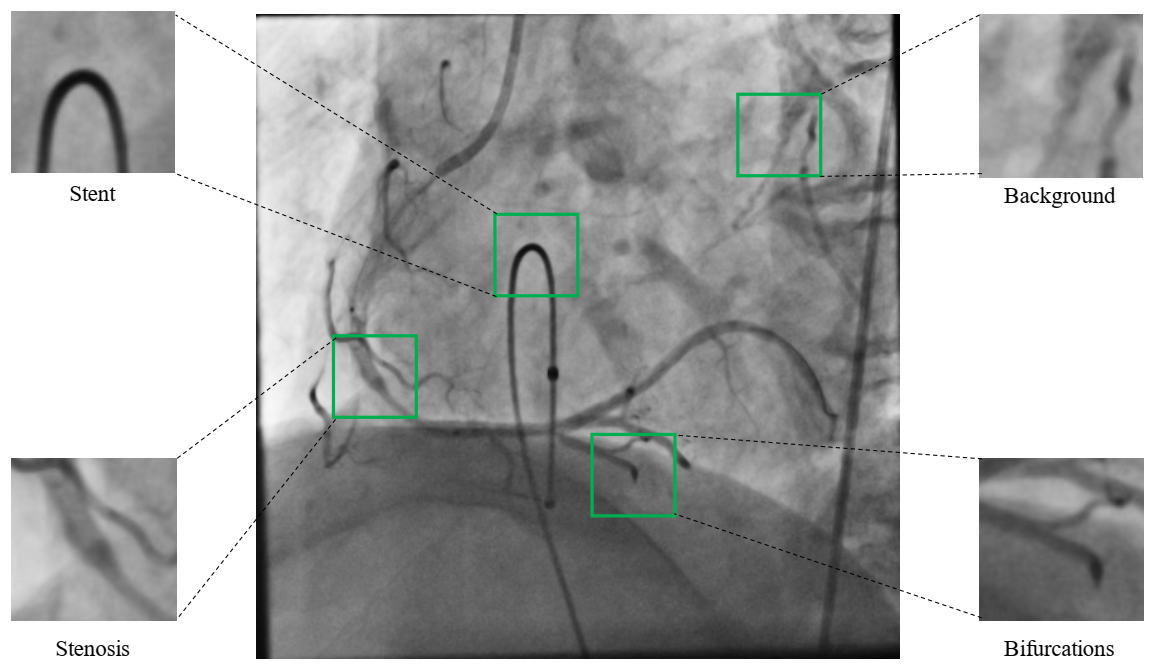
Moreover, the XCA screening test obtains high-resolution images of the main coronary arteries and their branches [6]. However, automatic stenosis detection is not easy due to the specific characteristics of XCA images, mainly background noise, the presence of a coronary stent, non-coronary vascular structures (i.e., ribs), and multiple superposed branching points [7,8,9], as shown in Figure 1.

Figure 1. XCA image with specific characteristics regions highlighted, such as a stent, background artifacts, coronary blood vessels with bifurcations, and stenosis cases.

In the last decade, CNNs have achieved outstanding performance gains in classification and segmentation tasks in the medical image domain compared with the traditional machine learning (ML)-based methods [10,11]. The core of CNN is its capability to extract, select, and classify features during the optimization step, while in ML methods, each of these steps is conducted independently. Different methods have been introduced to improve CNNs capabilities, such as attention mechanisms that adaptively recalibrate the intermediate feature maps by weighting their inter-channel and inter-spatial relationships; however, this increases the number of parameters of the network.

This paper proposes a Lightweight Residual Squeeze-and-Excitation Network (LRSE-Net) for stenosis detection. The proposed LRSE-Net model relies on Depthwise Separable Convolutions (DSC) [12] that have been shown to learn rich features with a reduced parameter set efficiently. Moreover, individuals improve the baseline architecture further.

2. Related Work

Machine learning techniques have been proposed to detect automatic stenosis in XCA images [13,14,15]. These studies first extract discriminative features based on texture and shape information. Then, a feature selection process is performed to choose the most suitable features to feed a classifier. Finally, different classifiers, such as Naive Bayes and Support Vector Machine, accomplish stenosis detection. However, features extracted in a hand-crafted manner limit the effectiveness of feature selection, and consequently, the classification performance.

Recently, deep learning methods have been able to tackle feature extraction, selection, and classification within the optimization procedure in an end-to-end manner, showing outstanding performance compared to the hand-extracted feature-based methods. Wu et al. [16] proposed a deep learning framework consisting of two stages. First, from the full raw XCA, candidate frames are selected based on the segmentation results that produce a UNet [17]. Subsequently, an object-based detection network employing a VGG (Visual Geometry Group) [18] as a backbone network provides the classification of stenosis regions. Following the same idea, Pang et al. [19] detected stenotic regions, including prior coronary artery displacement information. They used a Residual Network (ResNet) [20] that acts as a backbone model of the object detector network. Later, Danilov et al. [21] evaluated different object detection network configurations, including a Single Shot multi-box Detector (SSD) [22], Faster Region-Based Convolutional Neural Networks (Faster-RCNN) [23], and Region-based Fully Convolutional Networks (R-FCN) [24]. In their networks, distinct backbones networks have been employed, such as MobileNet-v2 [25], ResNet (50, 101) [20], and Inception-v4 [26].

However, the previous methods require the whole angiographic test and assume that a single stenosis region is present in the image. Another approach to solving this task is using a patch-based classification network. In this way, the full-size XCA image generates n-patches to be classified as positive or negative stenosis cases. In this context, Antczak and Liberadzki [27] employed a VGG-based model of only five convolutional layers to classify XCA image patches into the stenosis and no stenosis categories. A pre-training strategy was performed by synthetic data, consisting of a Bezier-based generative model to improve the results. Further, Ovalle-Magallanes et al. [28] proposed a novel hierarchical Bezier-based generative model to generate more realistic synthetic XCA patches. The dataset was evaluated on different ResNet configurations (18, 34, 50), including the Convolutional Block Attention Module (CBAM) [29]. Later, Ovalle-Magallanes et al. [30] performed an exhaustive evaluation of the impact of three attention mechanisms (Squeeze-and-Excitation [31], Convolutional Block Attention Module [29], and Efficient Channel Attention [32]). They demonstrated that a Trimmed ResNet18 with a Squeeze-and-Excitation attention module achieved the best trade-off between classification performance and computational cost. The methods mentioned above only employed a subset of the negative samples of the dataset released by Antczak and Liberadzki [33] to create a balanced training and test dataset; thus, only 125 negative and 125 positive cases were selected. This can lead to a biased classification when a large dataset is tested.

As discussed in previous paragraphs, different deep learning approaches have been used to develop strategies to detect stenosis in XCA images, through either object-based or patch-based models. These methods have shown notable performance; nevertheless, object-based approaches are limited to detecting a single stenosis case in the whole image. Meanwhile, patch-based methodologies are restricted to detecting small stenotic regions (i.e., based on the size of the patch). Moreover, both approaches take as their backbone network architectures designed for the ImageNet dataset, changing only the top of the model. Hence, redundant kernels may exist, limiting the classification performance.

This study presents a Lightweight Residual Squeeze-and-Excitation Network (LRSE-Net) for a patch-based stenosis classification based on two compression methods to reduce the model size: (1) redundant kernels deletion and (2) tensor decomposition by Depthwise Separable Convolutions. Additionally, they include independent ratios for each attention module to improve the feature extraction and generalization. The proposed LRSE-Net is up to $48\times$ smaller (in number of parameters) than previous models employed for this task. The network’s performance is evaluated employing two public datasets: (1) The full dataset from Antczak and Liberadzki [33] consisting of 1519 images with 125 positive cases of stenosis and the remainder as negative. (2) A patch-based version of the dataset released by Danilov et al. [34], which includes 6769 positive patches and 26,699 negative patches. The main contributions of this research are as follows:

• An LRSE-Net model is proposed by replacing vanilla convolutions with Depthwise Separable Convolutions, drastically reducing the number of parameters;
• Independent dilation ratios for each attention module are selected to enhance the network performance;
• Redundant kernels in the convolutional layers are removed to obtain a smaller model;
• A data augmentation policy is introduced to mitigate the imbalance of the dataset;
• A new patch-based dataset is released to validate the model performance.

3. Materials and Methods

The proposed LRSE-Net model consists of two main elements: a Squeeze-and-Excitation Attention Mechanism [31] and Depthwise Separable Convolution [12]. Altogether, these two modules produce robust stenosis detection by employing fewer parameters. In this section, a full description of these fundamental components is given.

3.1. Squeeze-and-Excitation Attention Mechanism

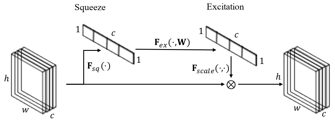
A Squeeze-and-Excitation (SE) block is a gating mechanism that models channel-wise feature relationships by integrating two operations: a squeeze operation and an excitation operation. In this manner, the network can enhance hierarchical features in a channel-wise manner. The structure of an SE block is illustrated in Figure 2.

Figure 2. Squeeze-and-Excitation block. The input features are recalibrated (${\mathbf{F}}_{scale}(·,·)$) by learnable weights (${\mathbf{F}}_{ex}(·,\mathbf{W})$) that capture the channel dependencies (${\mathbf{F}}_{sq}(·)$).

3.1.1. Squeeze Operation

In order to capture channel dependencies between the input feature maps $\mathbf{X}\in {\mathbb{R}}^{h\times w\times c}$, where $h\times w$ is the spatial size of the features and c is the number of channels, a Global Average Pooling (GAP) [35] calculates the global spatial information (squeeze) into a statistic $\mathbf{z}\in {\mathbb{R}}^c$. Each m-element of the statistic is given by:

$$z_m={\mathbf{F}}_{sq}\left({\mathbf{x}}_m\right)=\frac{1}{h\times w}\sum _{i=1}^h\sum _{j=1}^w{\mathbf{x}}_m(i,j).$$

(1)

Notice that this operation is parameter-free and applies a dimensionality reduction; thus, it reduces each feature map ${\mathbf{x}}_m\in {\mathbb{R}}^{h\times w}$ to a single scalar value $z_m$.

3.1.2. Excitation Operation

The excitation operation aims to reduce the channel-wise feature complexity and boost generalization. A simple gating mechanism $g(·,\mathbf{W})$ is applied to accomplish this task, such that:

$$\mathbf{s}={\mathbf{F}}_{ex}(\mathbf{z},\mathbf{W})=\sigma \left(g(\mathbf{z},\mathbf{W})\right)=\sigma \left({\mathbf{W}}_2\delta \left({\mathbf{W}}_1\mathbf{z}\right)\right),$$

(2)

where $\sigma$ and $\delta$ refer to the sigmoid and Rectified Linear Unit (ReLU) activation function, respectively, and noticing that ${\displaystyle \sum _{m=1}^c}{s}_m=1$. The gating mechanism acts as a bottleneck with two fully connected layers ${\mathbf{W}}_1\in {\mathbb{R}}^{c\times \frac{c}{r}}$ and ${\mathbf{W}}_2\in {\mathbb{R}}^{\frac{c}{r}\times c}$. Here, the parameter r is a reduction ratio controlling the number of parameters of the SE block. In such a way, a Squeeze–Excitation operation $\mathbf{SE}(·,\mathbf{W}):{\mathbb{R}}^{h\times w\times c}\to {\mathbb{R}}^{1\times 1\times c}$ can be defined as:

$$\mathbf{s}=\mathbf{SE}(\mathbf{X},\mathbf{W})={\mathbf{F}}_{ex}({\mathbf{F}}_{sq}\left(\mathbf{X}\right),\mathbf{W}).$$

(3)

Finally, the input feature maps $\mathbf{X}$ are weighted by the obtained values $\mathbf{s}$ to obtain a learnable recalibration that emphasizes or ignores specific channels. The rescaling procedure is performed by:

$${\widehat{\mathbf{x}}}_m={\mathbf{F}}_{scale}({\mathbf{x}}_m,s_m)=s_m{\mathbf{x}}_m,$$

(4)

where ${\mathbf{F}}_{scale}({\mathbf{x}}_m,s_m)$ is a channel-wise multiplication between the feature map ${\mathbf{x}}_m\in {\mathbb{R}}^{h\times w}$ and the scalar $s_m$.

3.2. Depthwise Separable Convolution

Let $f_{conv}(·,\mathbf{W}):{\mathbb{R}}^{h_1\times w_1\times c_1}\to {\mathbb{R}}^{h_2\times w_2\times c_2}$ be a standard convolution operation that takes as input ${\mathbf{X}}^{in}$ and produces ${\mathbf{X}}^{out}$ parameterized by the kernel $\mathbf{W}\in {\mathbb{R}}^{k\times k\times c_1\times c_2}$ computed as:

$${\mathbf{x}}_{c_2}^{out}(i,j)=f_{conv}({\mathbf{x}}_{c_1}^{in},\mathbf{W})=\sum _{u=1}^k\sum _{v=1}^k\sum _{m=1}^{c_1}{\mathbf{W}}_m(i,j)\ast {\mathbf{x}}_m^{in}(i+u,j+v),$$

(5)

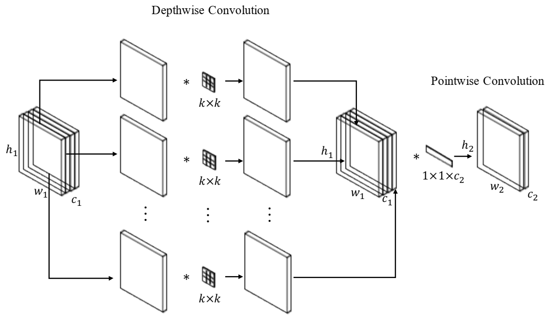
where ∗ represents the convolution operation and k—the filter size, Depthwise Separable Convolutions (DSC) factorize a standard convolution by two independent convolutions: (1) depthwise convolution and (2) point-by-point convolution (1 × 1 convolution), as shown in Figure 3. The depthwise convolution $f_{dw-conv}(·,\mathbf{W}):{\mathbb{R}}^{h_1\times w_1\times c_1}\to {\mathbb{R}}^{h_1\times w_1\times c_1}$ decoupled the input feature map from its channels, applying a single filter to each input channel, as follows:

$${\mathbf{x}}_{c_1}^{dw}(i,j)=f_{dw-conv}({\mathbf{x}}_{c_1}^{in},\mathbf{W})=\sum _{u=1}^k\sum _{v=1}^k{\mathbf{W}}_m(i,j)\ast {\mathbf{x}}_m^{in}(i+u,j+v).$$

(6)

Figure 3. Depthwise Separable Convolution. A standard convolution is factorized by a depthwise convolution and a point-by-point convolution.

Then, the pointwise $f_{pw-conv}(·,\mathbf{W}):{\mathbb{R}}^{h_1\times w_1\times c_1}\to {\mathbb{R}}^{h_2\times w_2\times c_2}$ convolution combines the features of each channel through a $1\times 1$ standard convolution, such as:

$${\mathbf{x}}_{c_2}^{out}(i,j)=f_{pw-conv}({\mathbf{x}}_{c_1}^{dw},\mathbf{W})=\sum _{m=1}^{c_1}{\mathbf{W}}_m\ast {\mathbf{x}}_m^{dw}(i,j).$$

(7)

This factorization reduces the number of parameters and computation operations.

3.3. Lightweight Residual Squeeze-and-Excitation Network

The proposed Lightweight Residual Squeeze-and-Excitation Network (LRSE-Net) consists of SE attention layers and DSC with residual connections layers. The network follows the structure of ResNet, where residual connections accelerate the training efficiency and resolve the gradient degradation problem. Formally, a residual block is defined as:

$${\mathbf{X}}^{out}=\delta \left({\mathbf{F}}_{res}({\mathbf{X}}^{in},{\mathbf{W}}_i)+{\mathbf{F}}_{down}({\mathbf{X}}^{in},{\mathbf{W}}_s)\right),$$

(8)

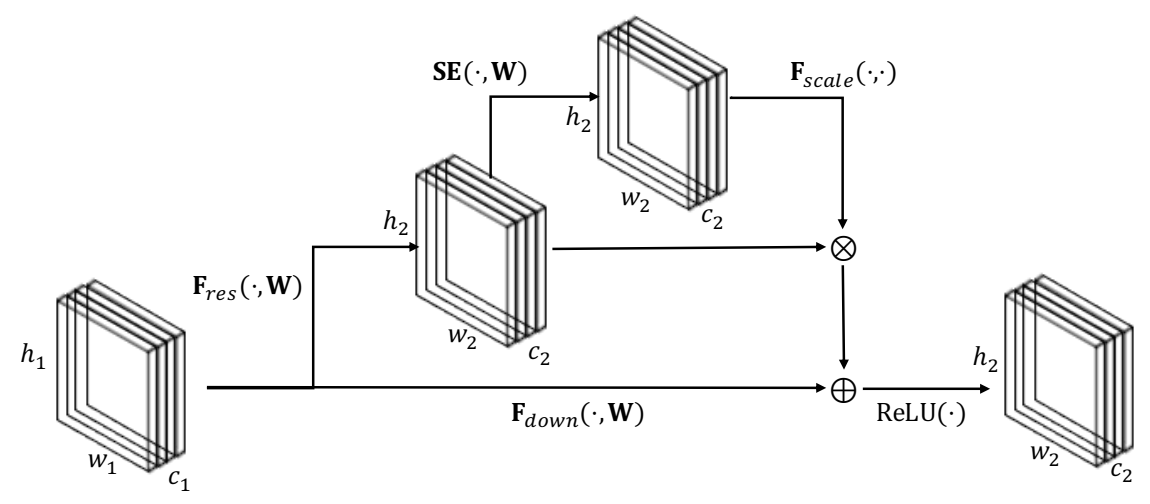
where ${\mathbf{X}}^{in}$ and ${\mathbf{X}}^{out}$ stand for the input and output feature maps, respectively, ${\mathbf{F}}_{res}(·,{\mathbf{W}}_i)$ represents the residual mapping to be learned parameterized by the kernels ${\mathbf{W}}_i$ i.e., multiple convolutional layers, ${\mathbf{F}}_{down}(·,{\mathbf{W}}_s)$ performs a linear projection with a learnable kernel ${\mathbf{W}}_s$ to match the dimensions (e.g., when the input/output channels changed), and $\delta$ is the ReLU function. The residual mapping follows the order of execution as Convolution → Batch Normalization → ReLU → Convolution → Batch Normalization. Note that the standard convolution is replaced with DSC. After the residual block, a SE attention module is placed to highlight key channel-wise information. Thus, the Residual Squeeze-and-Excitation $\mathbf{RSE}:{\mathbb{R}}^{h_1\times w_1\times c_1}\to {\mathbb{R}}^{h_2\times w_2\times c_2}$ block is defined as:

$$\mathbf{RSE}=\delta \left({\mathbf{F}}_{scale}({\mathbf{X}}^{res},\mathbf{SE}({\mathbf{X}}^{res},\mathbf{W}))+{\mathbf{F}}_{down}({\mathbf{X}}^{in},{\mathbf{W}}_s)\right),$$

(9)

where ${\mathbf{X}}^{res}={\mathbf{F}}_{res}\left({\mathbf{X}}^{in}{\mathbf{W}}_i\right)$ is the output of the residual mapping and $\delta$—the ReLU activation function. Figure 4 depicts an illustration of the Residual Squeeze-and-Excitation block.

Figure 4. Residual Squeeze-and-Excitation block. After the residual block, the SE attention module is placed to weight enhance the feature representation.

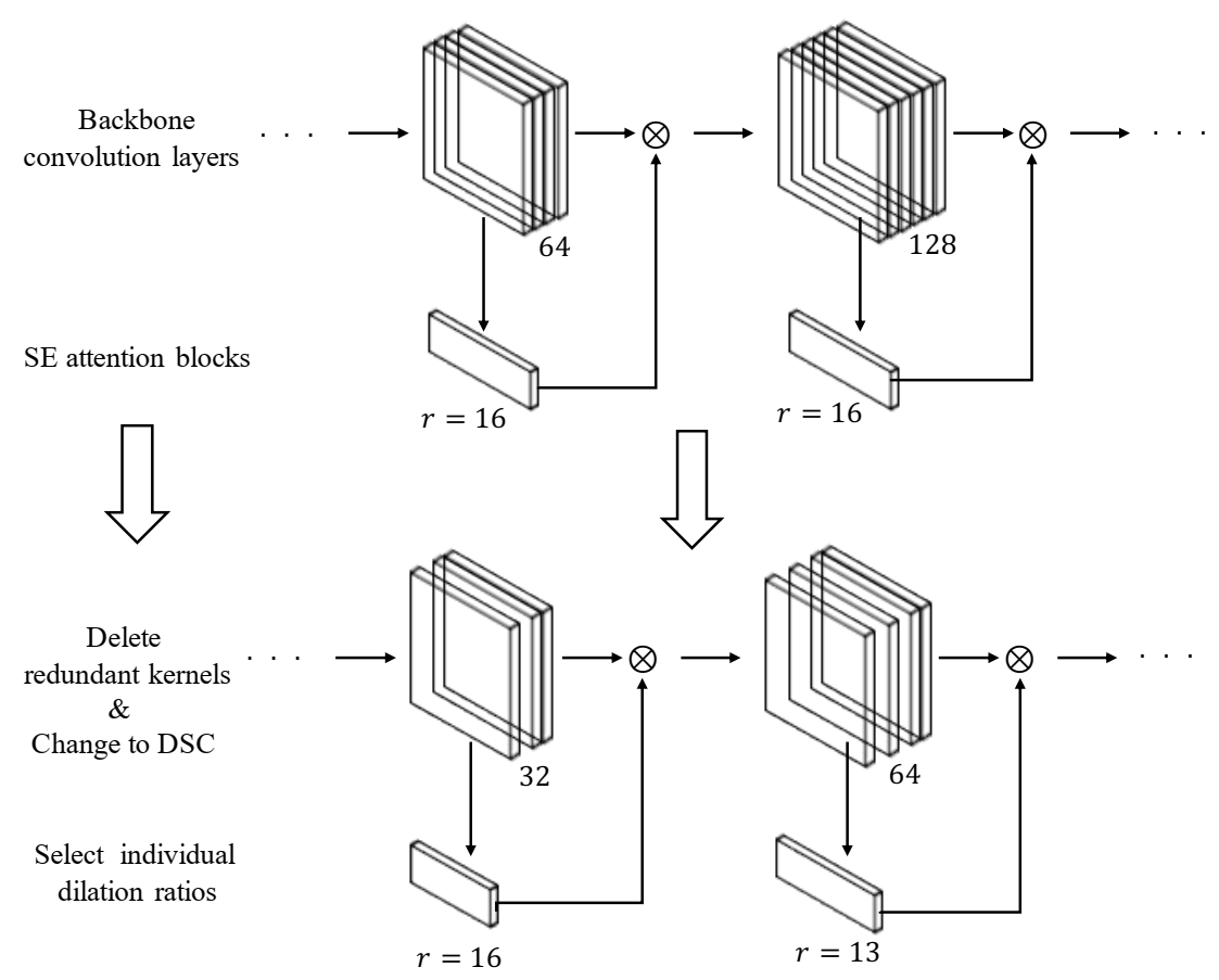
The proposed network took as a backbone network the ResNet18, which is mainly characterized by consisting of one $7\times 7$ convolutional layer, with a stride of two pixels, followed by a max-pooling of size two; four residual blocks within 64, 128, 256, and 512 kernels, respectively, come after. Then, redundant kernels were removed in the convolutional layers (half of them) to obtain a smaller model. Similarly, the top residual block and the first max-pooling are removed. A pipeline illustrating these model compression steps is shown in Figure 5.

Figure 5. Model compression pipeline. Redundant kernels are removed in the convolutional layers and DSC replaces the vanilla convolution.

Hence, the LRSE-Net structure contains 14 convolutional layers organized as one $3\times 3$ convolution with 32 kernels and stride of two pixels, three residual SE blocks, each with two residual mappings followed by a SE module with dilation ratios $r=16,13,9$, respectively, forming 12 convolutions with 32, 64, 128 kernels of size $3\times 3$, and one dense layer for final classification. Notice that a GAP layer reduces the feature maps’ dimensionality to a 1D vector that feeds the dense layer. Table 1 summarizes the LRSE-Net architecture. The optimal selection of the hyperparameters of the SE blocks and the number of kernels per residual block were obtained using the Tree-structured Parzen Estimator (TPE) algorithm [36,37], minimizing the validation Cross-Entropy Loss.

Table 1. LSRE-Net architecture. The dilation ratio r of the SE sub-module of the RSE block is specified. The input sample size is a $32\times 32$ and $64\times 64$ image patch.

Layer	Kernel Size	Stride	Output Size
Conv1	$\left[\begin{array}{c}3\times 3,32\end{array}\right]\times 1$	1	$32\times 32$/$64\times 64$
RSE 1	$\left[\begin{array}{c}3\times 3,32\\ 3\times 3,32\end{array}\right]\times 2$	1	$32\times 32$/$64\times 64$
	$r=16$	–
RSE 2	$\left[\begin{array}{c}3\times 3,64\\ 3\times 3,64\end{array}\right]\times 2$	2	$16\times 16$/$32\times 32$
	$r=13$	–
RSE 3	$\left[\begin{array}{c}3\times 3,128\\ 3\times 3,128\end{array}\right]\times 2$	2	$8\times 8$/$16\times 16$
	$r=9$	–
GAP	–	–	$1\times 128$
SoftMax	–	–	2

3.4. Datasets

Two public datasets were used to evaluate the proposed model: the Deep Stenosis Detection Dataset (DSDD) [33] and the Angiographic Dataset for Stenosis Detection (ADSD) [34].

DSSS [33] consists of small XCA image patches of size $32\times 32$ taken from different image positions and sources. It contains a total of 1519 images, where only 125 are positive cases of stenosis and 1394 negative cases, which generate an unbalanced ratio of 1:11, i.e., one positive case for eleven negative ones. This database does not specify a partition for training and testing sets.

ADSD [34] presented a set of XCA images with a total of 8325 grayscale images (100 patients) of $512\times 512$ to $1000\times 1000$ pixels. XCA images were taken using Coroscop (Siemens) and Innova (GE Healthcare) image-guided surgery systems at the Research Institute for Complex Problems of Cardiovascular Diseases (Kemerovo, Russia). A bounding box around stenotic segments was set with different areas: small (<322 pixels), medium ($322\le area\le 962$ pixels), and large (>962 pixels). The training and test subsets are specified with 7493 and 832 images, respectively.

A patch-based dataset was generated to evaluate the proposed patch-based approach from ADSD [34], taking square patches centered on the stenosis bounding box for the positive cases and the 4-connected neighbors around the bounding box as negative cases. During the patch selection, patches smaller than $32\times 32$ pixels were omitted. In this way, the new dataset (P-ADSD) consisted of 6769 positive patches, and 26,699 negative patches were obtained (1:4 unbalanced ratio). Thus, the training subset contained 6080 positive and 23,986 negative cases, while the test subset had 689 positive and 2713 negative cases. Patches were re-sized to $64\times 64$ to homogenize the image dimensions.

On the other hand, to deal with the small size of data with the unbalanced ratio of the DSSS [33], a data augmentation policy was applied, generating four additional images by input image. The policy includes random rotation around $90,180$, and 270 degrees, random horizontal flip, random horizontal and vertical shift of $-10\%$ to $10\%$, random zoom-in of $0\%$ to $10\%$, and random brightness change. Additionally, a partition of 80:20 was set to split the dataset into training and testing. The data augmentation policy was applicable only in the training and positive subsets. In this manner, the augmented dataset (A-DSSS), including 430 positive and 1394 negative stenosis cases, was obtained, reducing the unbalanced ratio to 1:3.

4. Results

The proposed LRSE-Net model was evaluated through multiple comparisons with different architectures employed for stenosis detection. The performance analysis was conducted using the datasets P-ADSD and A-ASSS described above. First, the evaluation metrics are defined. Secondly, the implementation details for training the model are explained. Finally, numerical results are shown.

4.1. Evaluation Metrics

For the evaluation of the proposed approach, five metrics are considered: Accuracy, Sensitivity, Specificity, Precision, and F${}_1$-score, which are defined as follows:

$$\mathrm{Accuracy}=\frac{\mathrm{TP}+\mathrm{TN}}{\mathrm{TP}+\mathrm{TN}+\mathrm{FP}+\mathrm{FN}},$$

(10)

$$\mathrm{Sensitivity}=\frac{\mathrm{TP}}{\mathrm{TP}+\mathrm{FN}},$$

(11)

$$\mathrm{Specificity}=\frac{\mathrm{TN}}{\mathrm{TN}+\mathrm{FP}},$$

(12)

$$\mathrm{Precision}=\frac{\mathrm{TP}}{\mathrm{TP}+\mathrm{FP}},$$

(13)

$$\mathrm{F}{}_1\text{-}\mathrm{score}=\frac{\mathrm{TP}}{\mathrm{TP}+0.5·(\mathrm{FP}+\mathrm{FN})},$$

(14)

where TP refers to the number of true positives, TN is the number of true negatives, FP denotes the false positives cases, and FN represents the number of false positives.

4.2. Implementation Details

The training process employs the Stochastic Gradient Descent with Momentum (SGDM) optimizer [38] with a learning rate of $1\times {10}^{-3}$ and a momentum of $0.9$. The model was trained with a batch size of 32 for 100 epochs minimizing the Cross-Entropy Loss. The model was implemented using the Pytorch framework, and the experiments ran on Google’s cloud servers, including a Tesla P4 GPU with 2560 CUDA cores and 8 GB of RAM.

To fairly compare the proposed method with other models, all the experiments followed the same hyperparameters and were initialized using the same seed. Moreover, a k-fold cross-validation (5-fold) was set following an 80:20 ratio from the validation subset. The validation step allows for saving the best weight during the training process. Table 2 summarizes the dataset partition distribution. Both dataset and their train–validation–test partition are freely available at: https://github.com/eovallemagallanes/LRSE-Net (accessed: 30 October 2022).

Table 2. Datasets partitions.

Dataset	Train		Validation		Test		Size
	Positive	Negative	Positive	Negative	Positive	Negative
P-ADSD	4864	19,188	1216	4798	689	2713	$64\times 64$
A-DSSS	385	892	20	223	25	279	$32\times 32$

4.3. Ablation Study

An ablation study over the A-DSSS dataset is presented to demonstrate the impact of the DSC, and the SE module is reported in Table 3. All configurations were trained from scratch employing the hyperparameters presented in the previous subsection. The comparative analysis evaluates four main groups of configurations: (1) without DSC and SE, (2) without DSC but with SE, (3) with DSC but without SE, and (4) with DSC and SE. For configurations using the SE module, two variants were tested: (1) with default reduction ratios ($r=16$) and (2) with independent ratios $r=16,13,9$. As mentioned before, the TPE algorithm was employed to find the model configuration minimizing the validation loss of the first fold.

Table 3. Ablation study on the A-DSSS dataset. The default SE ratio is 16 for each attention block.

DSC	SE	SE Ratios	Accuracy	Sensitivity	Specificity	Precision	F${}_1$-Score	# Params
✗	✗	N/A	0.9605	0.7600	0.9785	0.7600	0.7600	823,752
✗	✓	16, 13, 9	0.9605	0.7200	0.9821	0.7826	0.7500	829,128
		Default	0.9507	0.7600	0.9677	0.6786	0.7170	832,200
✓	✗	N/A	0.9540	0.7600	0.9713	0.7037	0.7308	224,744
✓	✓	16, 13, 9	0.9638	0.8800	0.9713	0.7333	0.8000	230,120
		Default	0.9638	0.7200	0.9857	0.8182	0.7660	233,192

Numerical results indicate that incorporating SE attention modules with individual reduction ratios increased Specificity and Precision compared with no attention model and default SE ratios and with a lower parameter addition. The exclusive use of DSC showed very competitive results in Accuracy, Sensitivity, and Specificity concerning the baseline model (with vanilla convolution operations). Still, it drastically reduced the number of parameters by around $3.6\times$. The DSC with SE, including default dilation ratios, achieved the best Specificity and Precision. In particular, including DSC and SE with individual reduction ratios presented the highest Accuracy, Sensitivity, and F${}_1$-score and the second-best required parameters, reducing the number of parameters by around $3.5\times$ compared to the baseline model. Therefore, this last model configuration was selected as the default model for subsequent comparison.

4.4. Stenosis Classification Performance Comparison

The performance of the LRSE-Net was evaluated on two public datasets (see Table 2). The methods trained all models from scratch and employed the same hyperparameters to ensure a fair comparison.

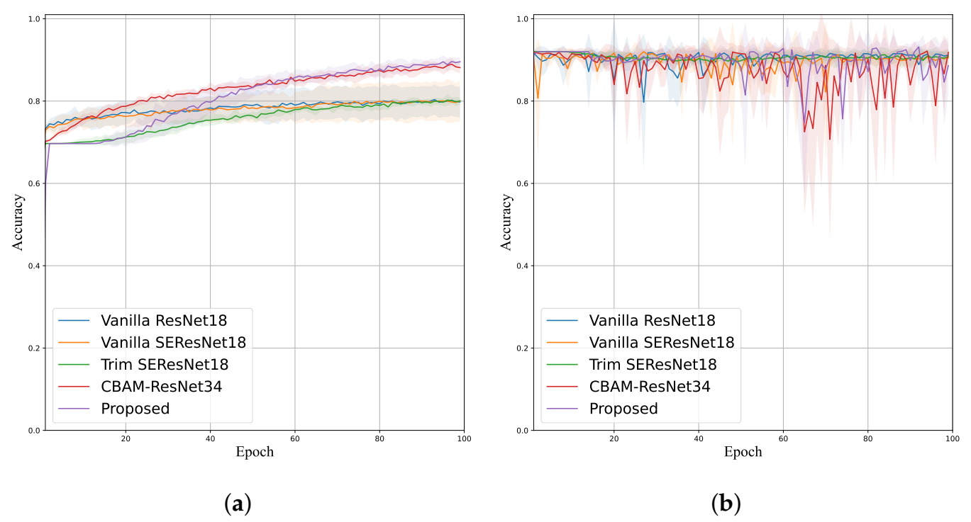
For the A-DSSS dataset, the results are shown in Table 4. It can be seen that the proposed LRSE-Net achieved the best mean Accuracy ($0.9349$), Sensitivity ($0.6320$), Precision ($0.5991$), and F${}_1$-score ($0.6103$). On the other hand, Vanilla ResNet18 achieved the best Specificity ($0.9850$). Even though LRSE-Net achieved $2.3\%$ less in Specificity concerning Vanilla ResNet18, it attained a gain of $2\%$, $50\%$, $13\%$ and $41\%$ in Accuracy, Sensitivity, Precision and F${}_1$-score. Compared with other attention models, Vanilla SE-ResNet18 obtained higher Specificity than the LRSE-Net, around $2\%$; however, Sensitivity, Precision, and F${}_1$-score were widely overcome by LRSE-Net. The training and validation curves are shown in Figure 6 and Figure 7, where it can be seen that the proposed model got the highest accuracy curves and the lowest loss. The second-best accuracy and validation curves are the ones of the CBAM-ResNet34. After 50 epochs, all validation losses started overfitting, showing up and down values due to the fold class imbalance. Notice that the validation subset is not augmented. The Trim ResNet18 achieved the most stable validation accuracy curve over the epochs.

Table 4. Performance comparison on the A-DSSS dataset.

Method	Accuracy	Sensitivity	Specificity	Precision	F${}_1$-Score	# Params
Vanilla ResNet18 [20]	0.9152 (±0.0071)	0.1360 (±0.0358)	0.9850 (±0.0069)	0.4661 (±0.1255)	0.2081 (±0.0492)	11,177,538
Vanilla SE-ResNet18 [31]	0.9172 (±0.0066)	0.1840 (±0.0607)	0.9828 (±0.0047)	0.4874 (±0.1082)	0.2652 (±0.0758)	11,267,650
Trim SE-ResNet18 [30]	0.8914 (±0.0040)	0.2000 (±0.0632)	0.9534 (±0.0057)	0.2729 (±0.0508)	0.2585 (±0.0474)	2,819,634
CBAM-ResNet34 [28]	0.9145 (±0.0062)	0.1920 (±0.0769)	0.9792 (±0.0069)	0.4529 (±0.0922)	0.2647 (±0.0817)	8,209,870
LRSE-Net (Proposed)	0.9349 (±0.0233)	0.6320 (±0.1820)	0.9620 (±0.0151)	0.5991 (±0.1161)	0.6103 (±0.1405)	230,120

Figure 6. (a) Training and (b) Validation accuracy curves of the A-DSSS evaluation.

Figure 7. (a) Training and (b) Validation loss curves of the A-DSSS evaluation.

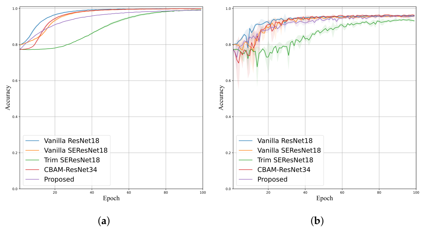
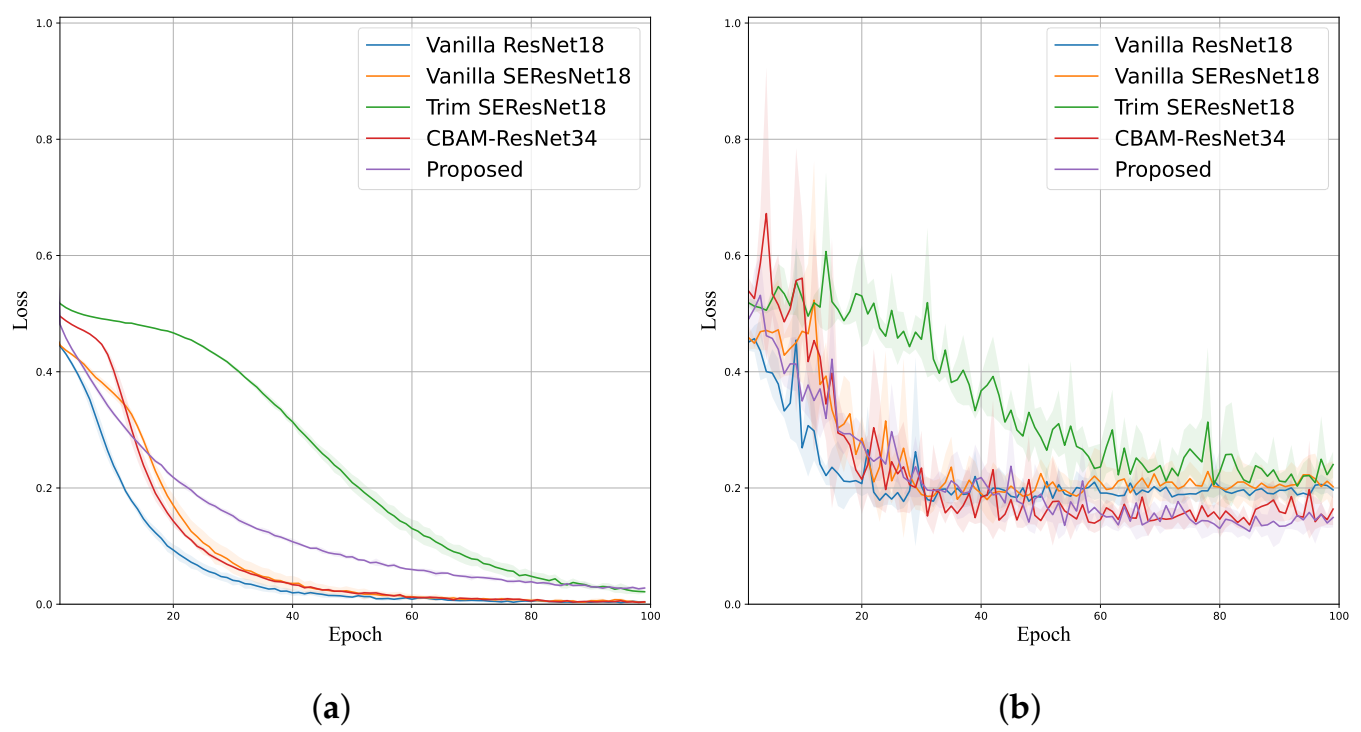
The performance employing the P-ADSD dataset is shown in Table 5. In this case, the proposed model achieved the best mean Accuracy, Sensitivity, Precision, and F${}_1$-score with $0.9543$, $0.8792$, $0.8944$, and $0.8863$, respectively; and the second-best Specificity with $0.9620$ (only $0.05\%$ below). Comparing the models within an attention mechanism, the proposed model had a gain in four evaluation metrics; CBAM-ResNet34 obtained the best Specificity, while Trim SE-ResNet performed poorly in Sensitivity ($0.7931$) and F${}_1$-score ($0.8134$). Their corresponding training and validation curves are shown in Figure 8 and Figure 9, confirming that the proposed model attained the lowest validation loss and higher validation accuracy than Trim-ResNet18 and Vanilla SE-ResNet18. The training curves exhibited a smoother behavior than the validation curves, where the LRSE-Net displayed lower accuracy and greater loss. Nevertheless, this leads to a better generalization performance.

Table 5. Performance comparison on the P-ADSD dataset.

Method	Accuracy	Sensitivity	Specificity	Precision	F${}_1$-Score	# Params
Vanilla ResNet18 [20]	0.9357 (±0.0054)	0.8139 (±0.0187)	0.9666 (±0.0056)	0.8614 (±0.0201)	0.8368 (±0.0135)	11,177,538
Vanilla SE-ResNet18 [31]	0.9403 (±0.0115)	0.8316 (±0.0278)	0.9679 (±0.0082)	0.8682 (±0.0323)	0.8494 (±0.0287)	11,267,650
Trim SE-ResNet18 [30]	0.9267 (±0.0065)	0.7913 (±0.0371)	0.9611 (±0.0046)	0.8380 (±0.0137)	0.8134 (±0.0204)	2,819,634
CBAM-ResNet34 [28]	0.9517 (±0.0046)	0.8647 (±0.0110)	0.9738 (±0.0035)	0.8936 (±0.0133)	0.8789 (±0.0113)	8,209,870
LRSE-Net (Proposed)	0.9543 (±0.0074)	0.8792 (±0.0246)	0.9733 (±0.0086)	0.8944 (±0.0301)	0.8863 (±0.0177)	230,120

Figure 8. (a) Training and (b) Validation accuracy curves of the P-ADSD evaluation.

Figure 9. (a) Training and (b) Validation loss curves of the P-ADSD evaluation.

Numerical results in both datasets demonstrate the efficacy of the proposed approach and indicate that SE modules with independent dilation ratios can enhance the feature representation, thus learning more discriminative features. Further, LRSE-Net accomplished better than the CBAM mechanism, which uses channel and spatial attention.

4.5. Class Activation Maps Compassion

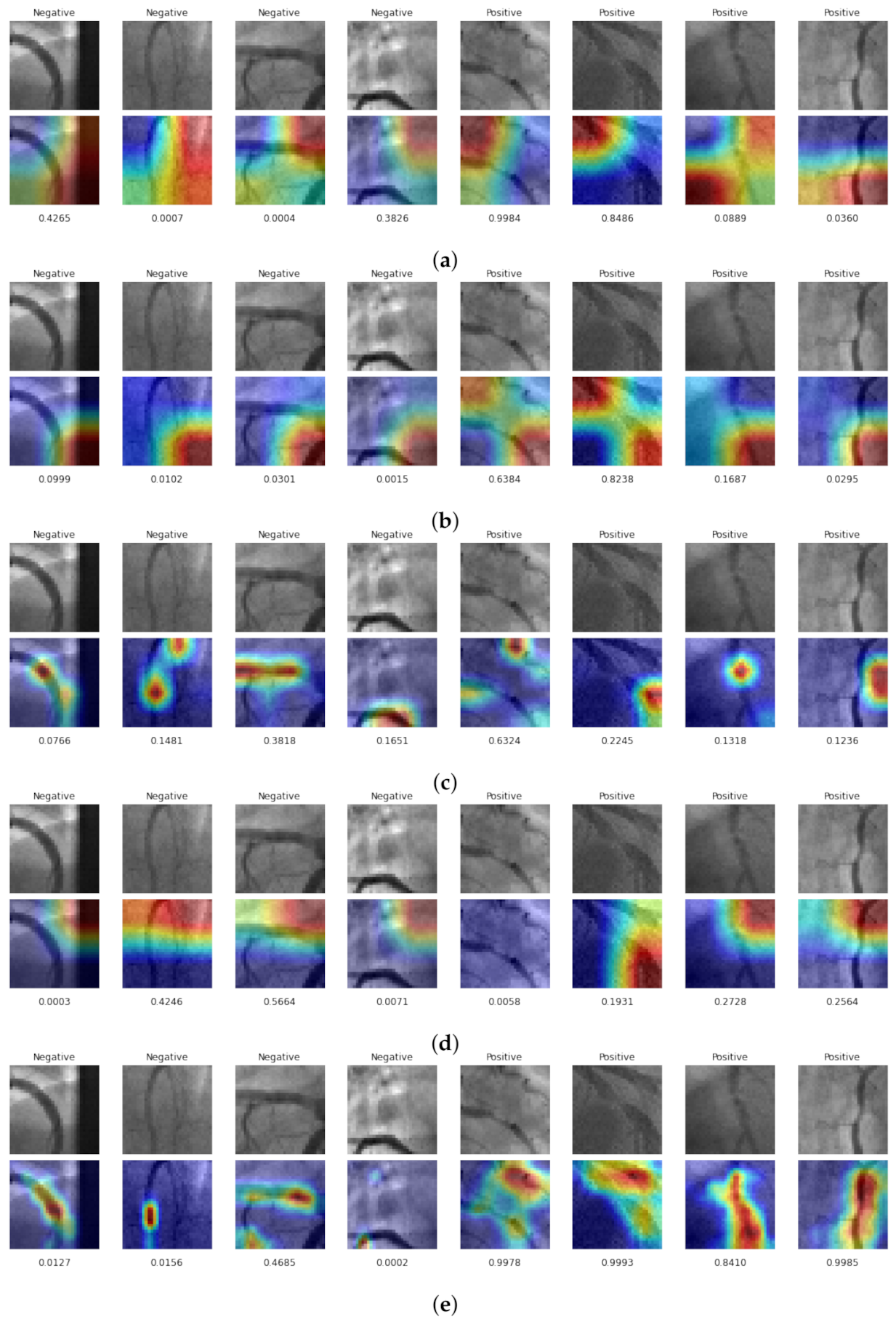
The Gradient-weighted Class Activation Map (GradCAM) [39] retrieves a visual explanation of the most important regions in the image for the model’s decision. Figure 10 illustrates the Grad-CAM for the test set of the A-DSSS dataset. High discriminative regions for stenosis detection are colored in hot tones (red colors) and cold tones (purple colors) for less informative regions (i.e., the gradient contributes in a minor way). In the model without attention (a) and including CBAM module (d), the GadCAM focused on corner regions more than blood vessel zones. For instance, the Vanilla ResNet18 showed two false negative cases in the last two test images; the CBAM-ResNet34 has one false positive (third row) and four false negative cases. In the case when the model includes the SE block (b), (c), and (e), the GradCAM started to set greater attention to blood vessel regions. The Vanilla SE-ResNet18 (b) arose a false positive case (first test image), the Trim SE-ResNet18 (c) an extra false negative (sixth column). In particular, the LRSE-Net presented greater attention over the blood vessel with non-false positive or negative cases.

Figure 10. The GradCAM responses for the test subset of the A-DSSS dataset. Four negative and four positive stenosis cases are shown. (a) Vanilla ResNet18, (b) Vanilla SE-ResNet18, (c) Trim SE-ResNet18, (d) CBAM-ResNet34, and (e) Proposed LRSE-Net. Red tones stand for high-attention regions, and purple for low-attention ones. Bellow each image, the probability of stenosis is set. For values higher than $0.5$, the models classify as stenosis cases.

As can be seen in Figure 11 for the P-ADSD dataset, the GradCAM featured more isolated high-attention regions in all the cases. These regions are located over blood vessel pixels for the Vanilla ResNet18 and the ResNet’s including SE block. In addition, the CBAM-ResNet34 (d) showed high attention to the positive stenosis cases in the background zones of the image.

Figure 11. The GradCAM responses for the test subset of the P-ADSD dataset. Four negative and four positive stenosis cases are shown. (a) Vanilla ResNet18, (b) Vanilla SE-ResNet18, (c) Trim SE-ResNet18, (d) CBAM-ResNet34, and (e) Proposed LRSE-Net. Red tones stand for high attention regions, and purple for low attention. Bellow each image, the probability of stenosis is set. For values greater than $0.5$, the models classify as stenosis cases.

The test images can include different blood vessel widths, background artifacts, and blood vessel bifurcations that affect the gradient activation regions. However, the GradCAM produced proper attention over the blood vessel for test cases with visible major blood vessels.

5. Discussion

The performance results validate the capability of the proposed method to classify stenosis cases in XCA image patches in different size datasets with major negative stenosis cases. Moreover, it was demonstrated that individual selection of dilation ratios for SE modules boosts the network performance. As the model goes deeper, the dilation ratios are smaller; this suggests that deeper features require an SE module with additional parameters to recalibrate the features. Similarly, the inclusion of DSC and the redundant kernel removal drastically reduced the network’s complexity (in terms of the number of parameters) up to $48.6\times$ compared with a vanilla ResNet18, $48.9\times$ concerning a vanilla SE-ResNet18, and $35.7\times$ smaller than the CBAM-ResNet34.

By visualizing training and validation curves, it can be seen that the network performance is directly affected by the quality and quantity of the training data. For example, the first dataset (A-DSSS) showed poor performance and rapid overfitting, even when data augmentation was performed. This scenario is not depicted employing the P-ADSD dataset, where around 33K images are available.

The GradCAM recovered a reasonable visual explanation over blood vessel regions, highlighting discriminative regions in hot tones and those with lower contributions in cold tones. Moreover, it supported the importance of incorporating an attention mechanism to improve the model numerical and explainable capabilities.

6. Conclusions

This paper proposed an LRSE-Net to classify stenosis cases from XCA images. The model consists of two main elements, a DSC and an SE module, which reflect high classification rates with lower computational requirements in terms of the required parameters. The proposed model is $48.9\times$ smaller than Vanilla SE-ResNet18 and $35\times$ smaller than CBAM-ResNet34. The experimental results demonstrate that LSRE-Net consistently outperformed Residual models with or without attention mechanisms. Additionally, the individual selection of dilation ratios for the SE blocks improved the classification performance, including a smaller dilation ratio as the network goes deeper. In particular, greater boosts were achieved when the dataset was small, with a gain of $2\%$, $50\%$, $13\%$, and $41\%$ in Accuracy, Sensitivity, Precision, and F${}_1$-score, respectively. Moreover, the LRSE-Net GradCAM maps retrieved a refined region proposal of the stenosis location, which could support the physician’s decision-making process.

Although the recognition rates are high, there is still a need for further improvements, such as evaluating the proposed model as the backbone for an object-based recognition system and detecting stenosis cases from the full XCA test. A future direction of this work concerning model compression may be to analyze other approaches, such as quantization, different low-rank-tensor decomposition, and knowledge distillation. Another research direction to address the limited training data could be generating artificial data by deep generative models.

References

1. World Health Organization. Cardiovascular Diseases (CVDs). 2022. Available online: https://www.who.int/health-topics/cardiovascular-diseases (accessed on 30 October 2022).
2. Britannica, The Editors of Encyclopaedia. Coronary Heart Disease. 2022. Available online: https://www.britannica.com/science/coronary-heart-disease (accessed on 30 October 2022).
3. National Heart, Lung, and Blood Institute. Atherosclerosis. 2022. Available online: https://www.nhlbi.nih.gov (accessed on 30 October 2022).
4. Nandalur, K.R.; Dwamena, B.A.; Choudhri, A.F.; Nandalur, M.R.; Carlos, R.C. Diagnostic Performance of Stress Cardiac Magnetic Resonance Imaging in the Detection of Coronary Artery Disease: A Meta-Analysis. J. Am. Coll. Cardiol. 2007, 50, 1343–1353. [Google Scholar] [CrossRef] [PubMed]
5. Athanasiou, L.S.; Fotiadis, D.I.; Michalis, L.K. Atherosclerotic Plaque Characterization Methods Based on Coronary Imaging; Academic Press: New York, NY, USA, 2017. [Google Scholar]
6. Johal, G.S.; Goel, S.; Kini, A. Coronary Anatomy and Angiography. In Practical Manual of Interventional Cardiology; Springer: Berlin/Heidelberg, Germany, 2021; pp. 35–49. [Google Scholar] [CrossRef]
7. Chiastra, C.; Iannaccone, F.; Grundeken, M.J.; Gijsen, F.J.; Segers, P.; De Beule, M.; Serruys, P.W.; Wykrzykowska, J.J.; van der Steen, A.F.; Wentzel, J.J. Coronary fractional flow reserve measurements of a stenosed side branch: A computational study investigating the influence of the bifurcation angle. Biomed. Eng. Online 2016, 15, 1–16. [Google Scholar] [CrossRef] [PubMed][Green Version]
8. Manson, E.; Ampoh, V.A.; Fiagbedzi, E.; Amuasi, J.; Flether, J.; Schandorf, C. Image noise in radiography and tomography: Causes, effects and reduction techniques. Curr. Trends Clin. Med. Imaging 2019, 2, 555620. [Google Scholar] [CrossRef]
9. Chang, C.F.; Chang, K.H.; Lai, C.H.; Lin, T.H.; Liu, T.J.; Lee, W.L.; Su, C.S. Clinical outcomes of coronary artery bifurcation disease patients underwent Culotte two-stent technique: A single center experience. BMC Cardiovasc. Disord. 2019, 19, 1–8. [Google Scholar] [CrossRef] [PubMed]
10. Sarvamangala, D.; Kulkarni, R.V. Convolutional neural networks in medical image understanding: A survey. Evol. Intell. 2021, 15, 1–22. [Google Scholar] [CrossRef] [PubMed]
11. Mohapatra, S.; Swarnkar, T.; Das, J. Deep convolutional neural network in medical image processing. In Handbook of Deep Learning in Biomedical Engineering; Elsevier: Berlin/Heidelberg, Germany, 2021; pp. 25–60. [Google Scholar] [CrossRef]
12. Chollet, F. Xception: Deep Learning with Depthwise Separable Convolutions. In Proceedings of the IEEE Conference on Computer Vision and Pattern Recognition (CVPR), Honolulu, HI, USA, 21–26 July 2017; pp. 1251–1258. [Google Scholar] [CrossRef]
13. Sameh, S.; Azim, M.A.; AbdelRaouf, A. Narrowed coronary artery detection and classification using angiographic scans. In Proceedings of the 2017 12th International Conference on Computer Engineering and Systems (ICCES), Cairo, Egypt, 19–20 December 2017; pp. 73–79. [Google Scholar] [CrossRef]
14. Wan, T.; Feng, H.; Tong, C.; Li, D.; Qin, Z. Automated Identification and Grading of Coronary Artery Stenoses with X-ray Angiography. Comput. Methods Programs Biomed. 2018, 167, 13–22. [Google Scholar] [CrossRef] [PubMed]
15. Kishore, A.N.; Jayanthi, V. Automatic stenosis grading system for diagnosing coronary artery disease using coronary angiogram. Int. J. Biomed. Eng. Technol. 2019, 31, 260–277. [Google Scholar] [CrossRef]
16. Wu, W.; Zhang, J.; Xie, H.; Zhao, Y.; Zhang, S.; Gu, L. Automatic detection of coronary artery stenosis by convolutional neural network with temporal constraint. Comput. Biol. Med. 2020, 118, 103657. [Google Scholar] [CrossRef] [PubMed]
17. Ronneberger, O.; Fischer, P.; Brox, T. U-Net: Convolutional Networks for Biomedical Image Segmentation. In Proceedings of the International Conference on Medical Image Computing and Computer-Assisted Intervention, Munich, Germany, 5–9 October 2015; Springer: Berlin/Heidelberg, Germany, 2015; pp. 234–241. [Google Scholar] [CrossRef]
18. Simonyan, K.; Zisserman, A. Very Deep Convolutional Networks for Large-Scale Image Recognition. In Proceedings of the 3rd International Conference on Learning Representations, ICLR 2015, San Diego, CA, USA, 7–9 May 2015; Conference Track Proceedings. Bengio, Y., LeCun, Y., Eds.; Cornell University: New York, NY, USA, 2015; pp. 1–14. [Google Scholar]
19. Pang, K.; Ai, D.; Fang, H.; Fan, J.; Song, H.; Yang, J. Stenosis-DetNet: Sequence consistency-based stenosis detection for X-ray coronary angiography. Comput. Med. Imaging Graph. 2021, 89, 101900. [Google Scholar] [CrossRef] [PubMed]
20. He, K.; Zhang, X.; Ren, S.; Sun, J. Deep Residual Learning for Image Recognition. In Proceedings of the 2016 IEEE Conference on Computer Vision and Pattern Recognition, CVPR 2016, Las Vegas, NV, USA, 27–30 June 2016; IEEE Computer Society: Los Alamitos, CA, USA, 2016; pp. 770–778. [Google Scholar] [CrossRef]
21. Danilov, V.V.; Klyshnikov, K.Y.; Gerget, O.M.; Kutikhin, A.G.; Ganyukov, V.I.; Frangi, A.F.; Ovcharenko, E.A. Real-time coronary artery stenosis detection based on modern neural networks. Sci. Rep. 2021, 11, 1–13. [Google Scholar] [CrossRef]
22. Liu, W.; Anguelov, D.; Erhan, D.; Szegedy, C.; Reed, S.; Fu, C.Y.; Berg, A.C. SSD: Single Shot MultiBox Detector. In Proceedings of the European Conference on Computer Vision, Amsterdam, The Netherlands, 11–14 October 2016; Springer: Berlin/Heidelberg, Germany, 2016; pp. 21–37. [Google Scholar] [CrossRef]
23. Ren, S.; He, K.; Girshick, R.; Sun, J. Faster R-CNN: Towards Real-Time Object Detection with Region Proposal Networks. In Proceedings of the Advances in Neural Information Processing Systems, Montreal, QC, Canada, 7–12 December 2015; MIT Press: Cambridge, MA, USA, 2015; Volume 28, pp. 91–99. [Google Scholar]
24. Dai, J.; Li, Y.; He, K.; Sun, J. R-FCN: Object detection via region-based fully convolutional networks. In Proceedings of the Advances in Neural Information Processing Systems, Barcelona, Spain, 5–10 December 2016; Curran Associates Inc.: Red Hook, NY, USA, 2016; pp. 379–387. [Google Scholar]
25. Sandler, M.; Howard, A.; Zhu, M.; Zhmoginov, A.; Chen, L.C. Mobilenetv2: Inverted Residuals and Linear Bottlenecks. In Proceedings of the IEEE Conference on Computer Vision and Pattern Recognition, Salt Lake City, UT, USA, 18–22 June 2018; pp. 4510–4520. [Google Scholar]
26. Szegedy, C.; Ioffe, S.; Vanhoucke, V.; Alemi, A.A. Inception-v4, Inception-ResNet and the Impact of Residual Connections on Learning. In Proceedings of the Thirty-first AAAI Conference on Artificial Intelligence, San Francisco, CA, USA, 4–9 February 2017. [Google Scholar]
27. Antczak, K.; Liberadzki, Ł. Stenosis Detection with Deep Convolutional Neural Networks. In Proceedings of the MATEC Web of Conferences; EDP Sciences: Les Ulis, France, 2018; Volume 210, p. 04001. [Google Scholar] [CrossRef]
28. Ovalle-Magallanes, E.; Avina-Cervantes, J.G.; Cruz-Aceves, I.; Ruiz-Pinales, J. Improving convolutional neural network learning based on a hierarchical bezier generative model for stenosis detection in X-ray images. Comput. Methods Programs Biomed. 2022, 219, 106767. [Google Scholar] [CrossRef] [PubMed]
29. Woo, S.; Park, J.; Lee, J.; Kweon, I.S. CBAM: Convolutional Block Attention Module. In Proceedings of the European Conference on Computer Vision, Munich, Germany, 8–14 September 2018; pp. 3–19. [Google Scholar] [CrossRef]
30. Ovalle-Magallanes, E.; Alvarado-Carrillo, D.E.; Avina-Cervantes, J.G.; Cruz-Aceves, I.; Ruiz-Pinales, J.; Contreras-Hernandez, J.L. Attention Mechanisms Evaluated on Stenosis Detection using X-ray Angiography Images. J. Adv. Appl. Comput. Math. 2022, 9, 62–75. [Google Scholar] [CrossRef]
31. Hu, J.; Shen, L.; Sun, G. Squeeze-and-Excitation Networks. In Proceedings of the IEEE Conference on Computer Vision and Pattern Recognition, Salt Lake City, UT, USA, 18–22 June 2018; pp. 7132–7141. [Google Scholar] [CrossRef]
32. Wang, Q.; Wu, B.; Zhu, P.; Li, P.; Zuo, W.; Hu, Q. ECA-Net: Efficient Channel Attention for Deep Convolutional Neural Networks. In Proceedings of the IEEE Conference on Computer Vision and Pattern Recognition, Seattle, WA, USA, 13–19 June 2020; pp. 11531–11539. [Google Scholar] [CrossRef]
33. Antczak, K.; Liberadzki, Ł. Deep Stenosis Detection Dataset. 2022. Available online: https://github.com/KarolAntczak/DeepStenosisDetection (accessed on 30 October 2022).
34. Danilov, V.; Klyshnikov, K.; Kutikhin, A.; Gerget, O.; Frangi, A.; Ovcharenko, E. Angiographic Dataset for Stenosis Detection; Mendeley Data, V2; Data Archiving and Networked Services (DANS): The Hague, The Netherlands, 2021. [Google Scholar] [CrossRef]
35. Lin, M.; Chen, Q.; Yan, S. Network in Network. arXiv 2013, arXiv:1312.4400. [Google Scholar]
36. Bergstra, J.; Bardenet, R.; Bengio, Y.; Kégl, B. Algorithms for Hyper-Parameter Optimization. In Proceedings of the Advances in Neural Information Processing Systems, Granada, Spain, 12–14 December 2011; Curran Associates Inc.: Red Hook, NY, USA, 2011; Volume 24. [Google Scholar]
37. Bergstra, J.; Yamins, D.; Cox, D. Making a Science of Model Search: Hyperparameter Optimization in Hundreds of Dimensions for Vision Architectures. In Proceedings of the International Conference on Machine Learning, Atlanta, GA, USA, 16–21 June 2013; Volume 28, pp. 115–123. [Google Scholar]
38. Qian, N. On the momentum term in gradient descent learning algorithms. Neural Netw. 1999, 12, 145–151. [Google Scholar] [CrossRef]
39. Selvaraju, R.R.; Cogswell, M.; Das, A.; Vedantam, R.; Parikh, D.; Batra, D. Grad-CAM: Visual Explanations from Deep Networks via Gradient-Based Localization. In Proceedings of the IEEE International Conference on Computer Vision (ICCV), Venice, Italy, 22–29 October 2017; IEEE Computer Society: Venecia, Italy, 2017; pp. 618–626. [Google Scholar] [CrossRef]
Publisher’s Note: MDPI stays neutral with regard to jurisdictional claims in published maps and institutional affiliations.
Article Metrics
Citations
Article Access Statistics
Multiple requests from the same IP address are counted as one view.