Abstract
Medical imaging is a complex process that capitulates images created by X-rays, ultrasound imaging, angiography, etc. During the imaging process, it also captures image noise during image acquisition, some of which are extremely corrosive, creating a disturbance that results in image degradation. The proposed work addresses the challenge to eliminate the corrosive Gaussian additive white noise from computed tomography (CT) images while preserving the fine details. The proposed approach is synthesized by amalgamating the concept of method noise with a deep learning-based framework of a convolutional neural network (CNN). The corrupted images are obtained by explicit addition of Gaussian additive white noise at multiple noise variance levels (σ = 10, 15, 20, 25). The denoised images obtained are then evaluated according to their visual quality and quantitative metrics, such as peak signal-to-noise ratio (PSNR) and structural similarity index (SSIM). These metrics for denoised CT images are then compared with their respective values for the reference CT image. The average PSNR value of the proposed method is 25.82, the average SSIM value is 0.85, and the average computational time is 2.8760. To better understand the proposed approach’s effectiveness, an intensity profile of denoised and original medical images is plotted and compared. To further test the performance of the proposed methodology, the results obtained are also compared with that of other non-traditional methods. The critical analysis of the results shows the commendable efficiency of the proposed methodology in denoising the medical CT images corrupted by Gaussian noise. This approach can be utilized in multiple pragmatic areas of application in the field of medical image processing.
1. Introduction
Medical imaging uses various processes and modalities to obtain images of different human body organs for diagnostic and therapeutic purposes. During this process, these images also capture unwanted artifacts, which require pre-processing, i.e., image denoising. The field of medical image denoising has seen rapid development over the past few decades to become a significant part of critical disease diagnosis [1]. Medical image processing and denoising observe a wide scale of applications which include: (i) brain tumor diagnosis and classification (from “benign” to “malignant”) using computed tomography (CT) and magnetic resonance imaging (MRI) scans, [2] (ii) treatment of craniofacial fractures with the help of ultrasound and CT scans, which includes 3D-imaging technology to produce high-quality images for orthopedic diagnoses, (iii) quick and accurate breast cancer detection followed by its classification from benign to malignant, (iv) diagnosis of congenital heart defects, (v) early detection of heart valve disorders, applying distinct techniques, such as electrocardiograms, chest X-rays, ultrasound imaging, Doppler techniques, and angiography, etc., (vi) accurate examination of tuberculosis and treatment for delimitating the spread of infection, (vii) detection of pathological brains by MRI scanning, and (viii) diagnosis of birth defects in babies. Medical image analysis includes multiple types of images, which vary based on how they are generated and appear. Each of them is corrupted by different types of noise, which degrade their image quality.
Ultrasonography is a well-established medical imaging technology, that applies high-frequency sound waves to analyze the structure of the different organs inside the human body [1]. Due to the back-scattering, a phenomenon that occurs when the ultrasound waves propagate through a biological medium, the images are contaminated with speckle noise, obfuscating the pertinent details and reducing the contrast of the soft tissues, thereby degrading their overall visual quality. Various filtering techniques and despeckling algorithms are applied, which include spatial domain filters during pre-processing and post-processing of images, such as a median filter, bilateral filter, Lee’s filter, Frost’s filter, squeezebox filter, Rayleigh maximum likelihood filter, and speckle-reducing anisotropic diffusion filter, and transform domain filters, consisting of wavelet thresholding-based, coefficients correlation-based, and Bayesian estimation-based techniques [3]. The computation complexity must be as low as possible since the despeckling of these images is done at run time. The medical diagnosis involving radiology testing, which uses magnetic fields and radio waves to produce 3D images, is widely known as magnetic resonance imaging (MRI), progressively becoming vital in clinical routine. Although relatively expensive, this technique produces detailed images of the structures of internal parts of the body, including the brain, spinal cord, bones and joints, heart, blood vessels, breast tissues, and other internal organs, with the help of MRI scanners and computers. The image quality is generally degraded by Rician noise [4]. The image denoising techniques should cover the aspects, such as edge-preservation and robustness to any artifacts, and some of the basic techniques include filtering methods, approaches of transform domain, statistical techniques, low-rank approximation, etc. Some of the notable ones that have been proven to be very effective in denoising Gaussian noise are the non-local means approach, wavelet sub-band coefficient mixing, unbiased kernel regression, block matching 3D, and so on. X-rays penetrate the body to create images of the different parts inside the body in variant shades of black and white, based on their distinct absorbance capacity. They are usually applied in computed tomography or CT scans [5].
The images produced are commonly corrupted by Poisson–Gaussian noise, which can be denoised using many different approaches, such as sinogram filtering techniques—including stationary wavelet transform, simple local average filtering, wiener filtering, and utilization of residual network during construction of CT images—iterative reconstruction techniques comprising of the total variation, non-local means approach, compressed sensing, 3D feature constrained reconstruction, and lastly, post-processing techniques involving artifact suppressing dictionary learning, discriminative feature representation, and low-rank recovery. Positron emission tomography (PET) is a procedure that involves nuclear imaging to provide information about the operation of different tissues and organs. These images are usually degraded by a low signal-to-noise ratio and blurred edges caused by Poisson–Gaussian noise, and for effective denoising, post-processing techniques are mandatory [5]. Some of them include local adaptive filtering, non-local means filtering, bilateral filtering, and the use of curvelets to achieve denoising. The research suggested treating the image and noise components equally and naturally transforming the image-denoising work into an image decomposition problem. To represent the noise and the medical image concurrently, they introduced a two-stage deep CNN-based image denoising [6]. This proposed method designed for edge preservation is different in terms of image decomposition. The study performs decomposition on the image and reduces the noise while in the proposed methodology; noisy components are classified separately and eliminated.
The main emphasis of this research has been set on the concept of method noise, which might seem to be a niche and not a well-exploited technique in the area of image processing but is a decade-old technique that focuses on edge preservations and specific image feature preservation while working with residual noise. It is usually used as a post-processing step to improve the resultant denoised image both in terms of qualitative, as well as quantitative, analysis [7]. The restoration of an image has shown exceptional results, and hence, the technique has the potential to be utilized in a wide range of applications, for example, medical image denoising, SAR image despeckling, digital image denoising, and so on. This paper presents a hybrid framework using the concept of method noise on a single-level basis with DnCNN for the denoising of medical CT images, which is a collection of deep neural networks and has shown cardinal efficacy in the field of image denoising due to the presence of well-trained neural preceptors via multiple layers [8].
1.1. Important Aspects That Contribute to the Degradation of the Overall Quality of CT Scan Images
CT picture quality depends on numerous things. Major image quality factors include:
- Blurring: Patient mobility might cloud CT reconstructions. Uncooperative patients, breathing, heartbeats, etc., might cause patient movement. The patient’s z-direction mobility complicates reconstruction techniques. Image reconstruction techniques use variable locations and spacing to simplify CT image reconstruction. However, patient z-direction movement should be regulated, since picture blurring relies on speed [9].
- (i)
- Equipment operation causes blurring.
- (ii)
- Correct procedure factors.
- (iii)
- Patient movement blurring.
- (iv)
- CT number variation between pixels for homogenous material scans.
- (v)
- Some noise-reduction filter techniques or incorrect settings blur the picture.
- Field of vision (FOV): A CT image reconstruction area. If a reconstructed CT picture is too tiny or large, it may be difficult to spot anomalies and reduce CT image quality [9].
- Artifacts: Unrelated picture distortion or inaccuracy. Artifacts are CT number discrepancies. Beam hardening, partial volume effect, metal artifacts, patient motion, etc.
- (i)
- Beam hardening: An X-ray beam traveling through the patient raises its average energy. Cupping describes this item. To prevent it, one can increase kvp, decrease slice thickness, pre-filter X-rays, avoid high-absorbing locations, and use appropriate algorithms.
- (ii)
- Metal artifact: Dental fillings, prosthetic devices, surgical clips, etc., may obstruct projection data and generate streaking artifacts. Any metal can be removed to lessen this artifact [10].
- (iii)
- Patient motion: Voluntary and involuntary movements may induce streaking in the reconstructed picture. Motion reduction, scan time reduction, immobilization, and placement assistance may help.
- (iv)
- Software and hardware-based artifacts: Poor software inputs and equipment may cause CT image artifacts. Mechanical failure, low gantry rigidity, mechanical assignment, aliasing, detector sampling, staircase, tube arcing, etc., might cause artifacts. Bad reconstruction parameterizations impair CT picture quality. The detector setup, tube current, tube potential, reconstruction method, patient placement, scan range, reconstructed slice thickness, and pitch may be optimized to enhance CT picture quality.
- Visual noise: Noise decreases picture quality. Acquisition, transmission, mathematical calculation, and voxel attenuation coefficient fluctuation may cause CT image noise. Visual noise degrades low-contrast items [10].
1.2. Major Contribution
The present study tried to improvise the result obtained in the study by Zhang et al., 2017 [11] by incorporating the concept of method noise as a post-processing operation. The study [11] presented an efficient CNN-based image denoising method on optical images. In the present study, an improvised methodology is adapted by adding method noise. This provides an improved result, and it majorly contributes to the following aspects:
- A CT image denoising technique is proposed using a hybrid combination of CNN and method noise. Here, method noise is applied as a post-processing operation.
- This hybrid denoising approach is specifically designed for better edge and fine details preservation.
2. Literature Review
Different types of medical images can be differentiated on the grounds of their appearance, the results they produce, and their applications. For instance, X-ray, computed tomography (CT), magnetic resource imaging (MRI), ultrasound, and positron emission tomography (PET) are some mundane examples of known and commonly used medical imaging techniques [12]. Deliberating the variegated types of medical images and their disparate characteristics in terms of resolution, speed, cost, and fundamental nature, different types of sound exist and thus require different types of image-denoising techniques. Although X-ray testing imageries are tinted by Poisson noise inheriting corruption characteristics from photon shot noise [12]; speckle noise is responsible for hampering the quality of ultrasound noise [13]. The detection of brain tumors of various categories has been done based on the analysis of magnetic resonance imageries by implementing a genetic bases algorithm amalgamated with an SVM machine [14]. The work shows promising results with accurate values when considering a particular type of brain tumor but is not tenable when working on different types of tumors by the application of the same methodology. WB filters have also been in the spotlight for achieving the same results from a different perspective [15]. Moreover, many authors chose to use concepts of wavelet decomposition for segmentation in MRI images [16] or implement SVM amalgamated with probabilistic neural network classifiers (PNNCs) in brain tumor tomography [17]. In contrast, the considered methodologies show tenable results in a particular niche category of brain tumor but fail to build robust mythologies that show equally promising results on other types of tumors. Additionally, some acumen for the field has been shown by authors, such as Elalfi et al. [18], on medical echocardiography imageries by utilizing attributes features from intensity histogram and gray level co-occurrence matrix (GLCM) utilized by the combined implementation of the backpropagation artificial network (BP ANN) and processing techniques, namely Gaussian filter and Gabor filter, to detect cardio muscular valve maladies. Though the work presents pristine results due to the complexity can be challenging to implement within limited computational power, storage, and time complexity.
Other hybrid approaches include work done by Somnath et al. [19], who propose a robust medical image denoising technique by optimizing the genetic algorithm via stochastic and randomizing the same, thereby segregating the image in fixed-sized blocks for wavelet transformation, showing the limited scope and appearing very insular or limited in nature. Handling speckle noise or denoising speckle noise in medical imageries has also shown esteem growth. Viswanath et al. [20] implement a combination of Gabor filter and artificial neural network (ANN) on ultrasound imageries to comprehend kidney abnormalities. Although the work presented is acute and precise for the considered data set, the scope of further application of the methodologies appears limited. Some groundbreaking work is done by combining the median filter and bilateral filter and comparing the results to median, wiener, and bilateral filters, thereby each pixel in an image is substituted to the weighted average of intensity values from proximity pixels, and a second filter is used to minimize the mean square error between the estimated values [21]. Thus, it has successfully developed and implemented a novel approach known as WB filters. Other methods that aim to improve the quality of medical images use a medley of speckle reduction methods and coherence enhancement techniques with total variation methods via wavelet shrinkage on ultrasound [22].
The literature on denoising speckle noise in medical images also includes hybrid approaches amalgamating bilateral filtering, wavelet thresholding, and transform domain [23]. The methodologies are effective and have multiple applications, but the presented work fails to display the various applications on the grounds of results and empirical implementation. Various techniques in medical image denoising that enhance the traditional approaches include work performed by author Gabriella [24], which alters the wavelet coefficient schema in the soft-threshold method, and this approach shows promising results and scope for future work with tenable empirical analysis. Moreover, sister denoising techniques in medical images that estimate noise variance and restore the images include pristine work done by proposing a robust and novel blind imagery [25], a deconvolutional technique inherited from noise variance estimation; this model primarily performs noise variance estimation and eventually restores images by least-square filter method using the previously estimated parameters at each gradation. Advanced denoising and image smoothing approaches include techniques proposed by author Chong [26], which address the issue of super-resolution imageries in medical images by the implementation of a hybrid approach, combining the use of a thin plate reproducing kernel Hilbert space (RKHS) and Heaviside functions. This method function of image smoothing, i.e., the edge smoothing, is performed by Heaviside functions, while RKHS performs others. Recently, CNN or convolutional neural network is being implemented amalgamated with various techniques, such as fuzzy c-means, k-mean, vector machine support, bilateral filters, FCM algorithms, and genetic algorithms, for exploring various uncharted grounds of the same [27,28,29]. The upcoming methods implementing convolutional neural networks include novel work done by residual noise learning as a learning methodology, along with batch normalization to obtain astute results on the ground of denoising and processing time, as analyzed by various matrices, such as PSNR, among others [30]. Heterogeneous medical image denoising poses a problem for various parochial denoising techniques that can be handled by implementing the combined approach of auto decoders and CNN to give robust, not precise results [31]. Another sister approach that leverages a supervised deep learning model [30], CycleWGANs, to improve low-dose PET image quality via the implementation of recently published deep learning methods (RED-CNN and 3D-cGAN) also provides efficient results, but its application is limited to PET scans.
Moreover, some latest state-of-the-art medical image denoising techniques include the use of a bio-inspired optimization-based filtering system implemented by CNN [32], where Gaussian and spatial weights influence the deliberation of medical images. The issue of robustness in medical image denoising and classification is addressed by [33,34], which successfully performs the task of image classification and denoising by amalgamating various CNN frameworks, naturally implanted auto-encoder, and high-level feature invariance at two sets of medical image tasks. The authors in [35,36,37,38,39,40,41] discussed image denoising-related techniques in multi-domains but related to the image. They have discussed reducing speckle noise from synthetic aperture radar images. They have discussed multi-focus and multi-modal image fusion keeping image deblurring in mind. A new image processing-based technique, C19D-Net, has been presented in work [42] to aid radiologists in improving their accuracy in identifying COVID-19 from chest X-ray (XR) pictures. Applying the InceptionV4 architecture and Multiclass SVM classifier, the proposed method extracts deep learning (DL) features to detect and categorize COVID-19 infections into four groups. In this study, we explore how to retrieve photos of plant leaves based on various attributes that have potential applications in the plant business [43]. Leaf types and diseases can be determined using a variety of picture attributes. A well-structured computer-assisted plant image retrieval strategy that can use a hybrid combination of the color and shape properties of leaf pictures for plant disease identification and botanical gardening in the agriculture sector is necessary for this aim [44].
3. Proposed Methodology
With the assumption that noisy CT images are corrupted by Gaussian probability distribution, a hybrid denoising method is proposed using method noise-based CNN. Here, a deep learning-based convolutional neural network (CNN) framework was implemented to address the corruption of medical images due to Gaussian noise. A pre-trained CNN that leverages deep learning architectures and image regularization methods were merged and custom fitted for this study [45]. This framework has been trained to denoise images contaminated with Gaussian noise, but unlike existing discriminatory models, this model is designed to handle unknown values of noise in the input image, making it markedly superior and more robust than its competitors. In this study, a hybrid technique implementing the “method noise-based CNN denoising approach” has been proposed. The state-of-the-art methodologies, in comparison with the proposed method, shows major decimation. The difference between the noisy image and the denoised image is the method noise (residual component). This often contains structural details and other minute artifacts that have been omitted due to imperfections or limitations of the denoising technique. By recovery followed by filtering of these fine details from the method noise and then adding them to the previous denoised image, the quality of the final denoised image could be further improved.
In this study, the cardinal usage of method denoising was applied to enhance the quality of medical images, specifically CT scan images. By successfully passing the image through ReLU and normalization filters, the neural network excludes important features, such as the sharpness of edges and proximity of pixels, that might be mundane to the algorithm but are palpable to the denoised image. By applying the method of noise-based CT image denoising, the denoised image was subtracted from the noisy image to generate the matrix representing the noise. On subsequent subtraction of the noise matrix from the noisy image, the loss of finer detail in the network is circumvented [46]. The Gaussian additive white noise (AWGN) is affixed to the original image at 1% to 2%. The noise is evenly distributed through the imagery plane with density values, following the normal distribution “bell curve”. Mathematically, the addition of Gaussian white noise can be shown as:
where i(x,y) is the original signal, n(x,y) is the added noise, and w(x,y) is the final image, with (x,y) determining the pixel location in the worldview plane. The bell curve follows a probabilistic distribution represented as:
where g represents the gray level, m is the mean or average of the function, and σ is the standard deviation of the noise. Its nature is such that even at the minuscule percentage of 0.1, the image quality is excessively corrupted. A brief overview of the proposed method using a flowchart is shown in Figure 1.
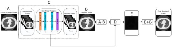
Figure 1.
Flowchart of proposed denoising method.
A brief description of the proposed methodology is summarized in below steps:
Step 1 (Input image): Read the input noisy CT image (A).
Step 2 (Perform CNN): Generally, given a CNN, denoted by A, having n architecture-related parameters λ1,…, λn whose decision spaces are Λ1,…, Λn, respectively, the CNN architecture design is to optimize the problem formulated as follows:
Here, λλ = {λ1,…, λn}, ΛΛ = Λ1 ×… × Λn, Aλλ denotes the CNN A adopting the architecture parameter setting λλ, and L(·) measures the performance of Aλλ on the validation data Dvalid after Aλλ has been trained on the training data Dtrain. In the case of classification tasks, L(·) measures the classification error of the tasks to which A is applied. Typically, gradient-based algorithms, such as stochastic gradient descent (SGD), are employed to train the weights of Aλλ, as L(·) is differentiable (or approximately differentiable), with respect to the weights. To optimize the CNN model, the following loss function is utilized for minimizing the error:
For the presented deep CNN architecture, the CNN network implemented has three layers, each different layer corresponding to a different function.
- Layer 1—Convolutional layers with ReLu, 64 filters each of dimensions 3 × 3 × [no. of channels] to produce 64 feature maps and rectified linear units.
- Channels for gray image = 1; Channels for color image = 3(RGB)
- Layer 2—Convolutional layers, ReLu with batch normalization by adding 64 filters to each of dimensions 3 × 3 × 64, such that batch normalization is added between each convolutional and ReLu layer.
- Layer 3—Final convolutional layer used for image reconstruction via 64 each filter of size 3 × 3 × 64.
In this model, two main features are used: the residual learning formulation is adopted to learn R(y), and batch normalization is incorporated to speed up training, as well as boost the denoising performance. By incorporating convolution with ReLU, CNN can gradually separate image structure from the noisy observation through the hidden layers. Such a mechanism is similar to the iterative noise removal strategy adopted in methods, such as EPLL and WNNM, but the CNN is trained to accommodate the entire process from start to end. The CNN is a deep-learning model trained to recreate the image while simultaneously removing the noise. In this model, not unlike other models, the layers perform three variants of complex computation as expounded. For a network of D depth, the first layer applies Conv + ReLU leveraging a sliding window, charting the features of the image into 64 convolution feature maps of lower dimensions, referencing ReLU as the activation function for non-linearity. The succeeding 2–(D-1) layers use an amalgamation of Conv + BN + ReLU to inflate the feature maps to the size of the image by inserting padding elements, following which feature mapping can be repeated. This process continues with convolution vector generation and pooling occurring in alternation whilst the last layer uses a filter of size 3 × 3 × 64 to reconstruct the denoised imagery. The input of each layer is the output of the preceding layer, hence, the prospect arises to implement residual learning, allowing for the exclusive removal of the remnants of the underlying clean image, thereby making the system generate consistent results impartial to the content of the image.
Step 3 (Method noise-based CNN): This is the most crucial section of this study. In this step, the method noise is extracted from the denoised image. Next, it is re-iterated into the DnCNN for refinement and recovery of any minuscule structural information that has been missed in the original denoising cycle. The output after this cycle gives the denoised counterpart of the method noise, which is superimposed on the previous denoised result to synthesize the outcome (Equation (3)).
Method noise implementation:
where a = original noisy image, and e = final denoised image
Step 4: D is the subtracted image that contains the residual component. Now apply CNN over a subtracted image (D) and obtain a filtered subtracted image (E).
Step 5: To get the final denoised image, perform addition between intermediate results as below:
F = E + B
F is the final denoised image.
4. Experimental Result and Analysis
4.1. Training Dataset
To train the model, 2500 images were extracted from the ELCAP Public Lung Image Database and utilized to simulate white Gaussian noise. The training images were divided into 603 individual 512 × 512 patches and saved as *.bmp files. The size of the patch was determined to be 65 × 65. The patch size was decided to be 65 × 65 for the following reasons: the designed network is comprised of two sub-networks, each of which has a depth of 17, the depth of BRDNet is 18, and the receptive field of one network is 2 times 17 plus one, which equals 35, while the receptive field of the other network is 61. If the patch size is going to be bigger than the size of the receptive field, the planned network is going to need extra computational cost. Nevertheless, the patch size is bigger than the receptive field size of the first network, which means that it can give supplementary information for the second network. Therefore, a patch size of 65 is appropriate to strike a balance between effectiveness and performance [47].
4.2. Testing Dataset
White Gaussian noise is used for the training of the denoising model in the process of gray-noise picture denoising. The authors of this study have selected the ELCAP Public Lung Image Database as their test dataset in accordance with the DnCNN and FFDNet methodologies. The dataset that was employed contains more than 2000 CT pictures, each of which is 512 pixels wide and 512 pixels high. Table 1 shows a qualitative result analysis of the proposed methodology using different performance metrics, i.e., PSNR and SSIM with different numbers of Epochs. The result analysis is tested over 2500 CT images with different numbers of epochs. The average result of PSNR and SSIM with the different number of epochs is shown in Table 1. Here, the authors observed that the best result of PSNR and SSIM is obtained with 30 epochs. Hence, for the proposed methodology, we tested all results with 30 epochs [48].

Table 1.
Performance metrics with different epochs.
In this section, the experimental results of the proposed method over noisy CT images with their performance aspects are presented. All the experiments are performed on the standardized and simulated CT image data set with artificially introduced white Gaussian noise. Additionally, qualitative, quantitative, and graphical analysis is done to provide evidence for the efficacy of the proposed method. The reference CT image dataset is shown in Figure 2. The CT images are of [512 × 512] resolution size, which is used for consistency. This framework can work with dynamic image size, and performance commensurate to the available hardware. The image shown in Figure 2d refers to grayscale using built-in MATLAB functions before use.
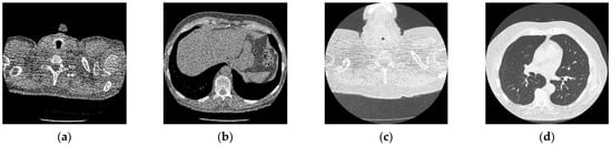
Figure 2.
Online access database of original CT images [49]; (a) Reference CT1 image; (b) Reference CT2 image; (c) Reference CT3 image; (d) Reference CT4 image.
4.3. Qualitative Analysis
Figure 3 shows the corruption of a CT image after the addition of 20% Gaussian noise. The degradation in image quality is visible to the naked eye without aid when compared to the original CT image. Figure 4, Figure 5, Figure 6, Figure 7, Figure 8, Figure 9, Figure 10 and Figure 11 show the denoised CT images, corresponding to CT images in Figure 3 and generated from various denoising models. The results show a discernible reduction in both the gaussian noise introduced, as well as the noise present in the original CT image whilst safeguarding the finer details present in it.
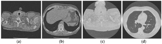
Figure 3.
Noisy CT image data set after inserting 20% noise); (a) Noisy CT1 image; (b) Noisy CT2 image; (c) Noisy CT3 image; (d) Noisy CT4 image.

Figure 4.
Result of CNN for X-ray low-dose CT image denoising method [21]; (a) Denoised CT1 image; (b) Denoised CT2 image; (c) Denoised CT3 image; (d) Denoised CT4 image.
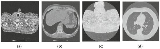
Figure 5.
Result of block matching CNN-based image denoising method [22]; (a) Denoised CT1 image; (b) Denoised CT2 image; (c) Denoised CT3 image; (d) Denoised CT4 image.
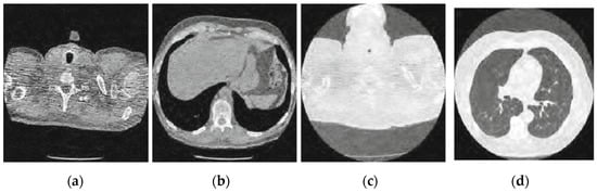
Figure 6.
Result of enhanced CNN-based image denoising method [23]; (a) Denoised CT1 image; (b) Denoised CT2 image; (c) Denoised CT3 image; (d) Denoised CT4 image.
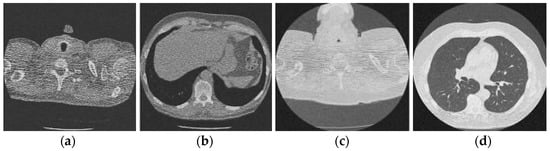
Figure 7.
Result of image denoising method using CNN with batch renormalization [35]; (a) Denoised CT1 image; (b) Denoised CT2 image; (c) Denoised CT3 image; (d) Denoised CT4 image.
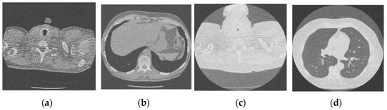
Figure 8.
Result of image denoising method using enhanced Hilbert space technique [45]; (a) Denoised CT1 image; (b) Denoised CT2 image; (c) Denoised CT3 image; (d) Denoised CT4 image.
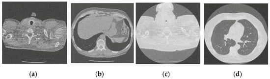
Figure 9.
Result of image denoising method using CNN based on residual learning approach [46]; (a) Denoised CT1 image; (b) Denoised CT2 image; (c) Denoised CT3 image; (d) Denoised CT4 image.
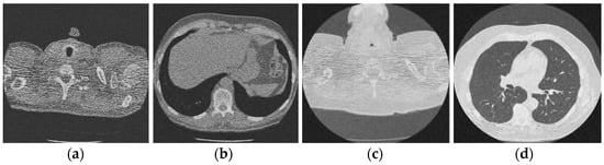
Figure 10.
Result of image denoising method using CNN autoencoders [47]; (a) Denoised CT1 image; (b) Denoised CT2 image; (c) Denoised CT3 image; (d) Denoised CT4 image.
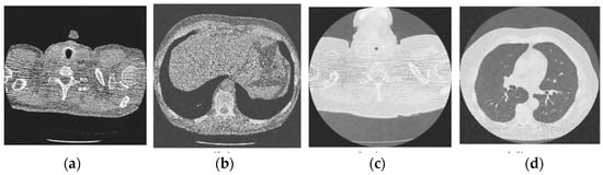
Figure 11.
Results of the proposed CT image denoising method; (a) Denoised CT1 image; (b) Denoised CT2 image; (c) Denoised CT3 image; (d) Denoised CT4 image.
For effective comparison to other systems available out there, this system has been pitted against seven of the most robust and widely used denoising techniques out there, i.e., Figure 4, Figure 5, Figure 6, Figure 7, Figure 8, Figure 9, Figure 10 and Figure 11. All the denoising frameworks performed reasonably well, with similar levels of denoising in their outputs, within a certain margin of error and variations. The result from these techniques for four CT images is displayed in Figure 4, Figure 5, Figure 6, Figure 7, Figure 8, Figure 9, Figure 10 and Figure 11. The CT image manipulation gave rise to redundant overcorrection, cumulating in distortion of the black borders and the introduction of fuzziness. Only two CT images from the rivaling systems have managed to preserve the blackness of the outer borders in the CT images. The result from [45] in Figure 9c is the least clear, with distortion visible to the unaided observer. A similar problem is observed in Figure 4a,c, where the system overcorrects, introducing more distortion instead of improving clarity. Figure 10d comes closest to the original, though the proposed framework is superior, as illustrated in the next section. From Figure 11a–d, it is very clear that the proposed algorithm gives better outcomes in comparison to existing methods in terms of clinical features, such as edges, textures, contrasts, and brightness.
Figure 12 and Figure 13 analyze the region of 45 × 45 that has been considered to be the upper right area of the center in a region containing all types of details, including edges, shade gradient, and extremities, in contrast values. This region was mapped in the same area for all the noisy and denoised CT images using built-in MATLAB functions. Post this, magnification shows the edge reconstruction and contrast restorative properties of this framework in grandiose detail in Figure 14. The white regions of details are visible with a high level of clarity in the denoised CT images in Figure 14. The Gaussian noise is also clearly visible in the magnified view, as seen in Figure 14a–c. The recovery from Figure 14c is beyond the capability of any human expert, which is done flawlessly by the system.
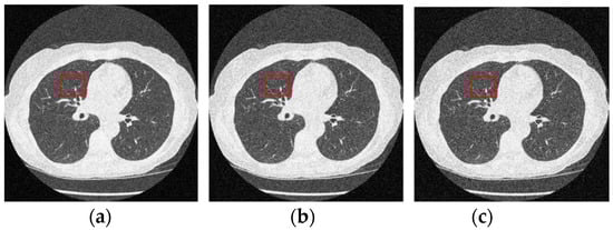
Figure 12.
Noisy CT images with various noise variance levels (a) 1% Gaussian noise, (b) 1.5% Gaussian noise, and (c) 2% Gaussian noise.
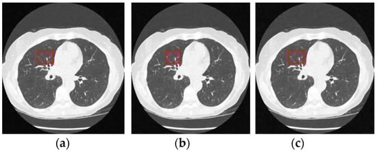
Figure 13.
Denoised CT images generated via proposed technique: Marked region used for zooming analysis; (a) denoised on 1% Gaussian noise, (b) denoised on 1.5% Gaussian noise, and (c) denoised on 2% Gaussian noise.
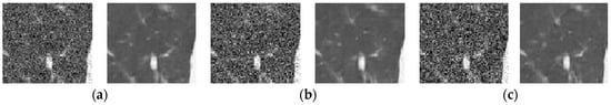
Figure 14.
Comparison of the marked region from noisy and denoised CT images: Zooming analysis of the marked region. (a) 1% Gaussian noise, (b) 1.5% Gaussian noise, and (c) 2% Gaussian noise.
4.4. Quantitative Analysis
To validate the proposed algorithm via empirical means, comparisons have also been made based on CT image metrics. Two of the most widely used reference-based matrix, namely PSNR and SSIM, formed the groundwork for valuational criteria. These PSNR and SSIM values for the four CT scan images are compiled in Table 2 and Table 3, respectively. Each system has worked on 16 cases, corresponding to four progressively greater noises. On comparing the different values, it is clear beyond a shred of doubt that the proposed framework outperforms its competitors in 100% of the cases considered. In engineering, PSNR refers to how well a signal is preserved, relative to how much its representation has been tainted by noise. The higher the PSNR value, the better the denoised image is considered. SSIM is a perceptual metric that measures how much impact operations, such as data compression or transmission losses, have on an image’s perceived quality. The range of SSIM lies between 0 and 1. The nearer value to 1 is considered as better denoising.
Table 2.
PSNR values of the proposed method with other compared methods.
Table 3.
SSIM values of the proposed method with other compared methods.
For PSNR, increase in noise by 0.5% proliferated a decrease of 2–3 points in PSNR. This result is consistent among all results for all four CT images. Considering the case of SSIM, only [45] was close to the proposed framework with a 0.0020, while lower noise levels subsequently lagged further behind at a gap of 0.0400 at higher noise levels. The maximum difference of 0.24 gives it an amazing score increase of around 24%. Overall [35] had lower PSNR scores than the rest, with a minimum of 1 point lower than the others. [35] had the lowest value of 20.97 for CT image no.4 at 25 noise variances; this is considered substandard and might arise due to unknown factors. [21,45] have PSNR values closer to the proposed technique at a noise of 5, but the difference increased for higher noise values.
SSIM was calculated for cases with . Although the difference is not prominent at first glance due to the range limit from 0 to 1, a trend similar to the case of PSNR is seen. However, the difference between the proposed framework and the outcome of [21,45] has widened: SSIM [45] as quite a bit inferior to the proposed technique [35] performs least favorably, it has a 19.19% difference in CT image no.2 at when compared to the method denoising. The CT images with values greater than 0.70 can be considered fully understandable, which has been achieved on the majority of occasions. From Table 2 and Table 3, it is very clear that the proposed algorithm gives better outcomes in comparison to existing methods in terms of PSNR and SSIM.
To check the execution time, the existing methods and proposed method are evaluated over 187 noisy CT images. The average execution time is measured and shown in Table 4. From Table 4, it is clearly shown that the proposed method gives fast execution from other methods.
Table 4.
Average execution time (over 187 CT images) for different denoising methods (in seconds).
4.5. Graphical Analysis
The intensity profile is a quintessential tool for understanding the quality of CT images. They aid in analyzing the overall quality and document the number of pixels corresponding to a grayscale value, providing an easy-to-understand representation of CT image data at a glance. Furthermore, the similarity of two CT images can be visualized as a function of the overlapping on their intensity profile plots. Such an approach has been used in this case to verify the closeness of the denoised CT image to the original, regarding the number of pixels possessing the same grayscale value. Figure 15 shows the intensity profile of four CT images for noise values of = 5, 10, 15, respectively. The intensity profile, one for the denoised CT image and one for the original CT image, are plotted together in every graph. In Figure 15, the line for original and denoised CT images almost overlap throughout with little shift in some regions giving evidence of the integrity of the restored CT image. Similar results are shown in all other graphs, with no discernible change in the mean distance between the two lines at different noise values. This proves that the system works remarkably well throughout the entire range.
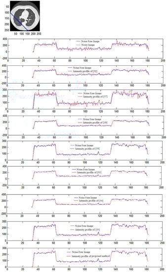
Figure 15.
Intensity profile of noise-free and denoised CT image of different methods: plotting the intensity [17,18,19,32,33,34,35].
In CT scan image 1, a large portion of the picture is white; hence, the number of pixels in the region near the start of the graph is more in Figure 15. A similar case has been observed in CT images no.2 and 3 accounting for the almost flat lines. However, although original values have not been restored, an attempt was made by the framework, as evident from the secondary peak near the lower (white) pixel values.
The intensity profile is a visual representation of the image in terms of the number of pixels between 0 to 255. The pixel with a darker gray shade has a lower value closer to 0 than a brighter pixel closer to the right end of the scale. The number density of pixels of any image is entirely dependent on the type of image; images shot in low light will have darker pixels in a larger number, while pictures shot outdoors under the sun will have the majority of values along a line segment of the CT image depicted on top of these image pixels of a higher value. This conglomeration of pixels in a particular range is represented as spikes in the intensity profile, which bear no influence on the performance of the denoising technique. The denoising algorithm corrects the noisy pixels based on the values of surrounding pixels and hence will be equally unperturbed by the type of image or the type of spikes in the intensity profile. The unnaturally large spike at the left side of the intensity profile is due to the presence of many pixels that are nearly black from the background of the CT or X-ray images. The presence or absence of noise will have a negligible impact on this factor and hence does not impact the performance or evaluation of the denoising systems.
5. Conclusions
It has been observed that noise removal from CT images has always been a critical step in medical image processing, and rapid improvements have been made in CT image denoising over time. This paper has presented a novel framework in CT image denoising, consisting of the state-of-the-art Single-Level Method of Denoising with the implementation of CNN, which can be efficiently applied to medical images. The process comprises adding additive white Gaussian noise to the medical image, and the noisy CT image generated as a result is then denoised using the CNN model. The remaining method noise is extracted from the denoised CT image and re-iterated in the CNN model for refinement. The resultant denoised counterpart is superimposed on the previous denoised result to obtain the final refined CT image. A detailed qualitative analysis was conducted in which two CT image quality metrics, the PSNR and SSIM, were applied for a comparison of the proposed technique with the other standard denoising techniques. The results generated exhibited that the proposed framework had scores superior to other state-of-the-art techniques, thus, validating its enhanced performance and reliability. Furthermore, an intensity profile is plotted between the original and the denoised CT image, in which the extremely marginal divergence between the plotted lines was truly indicative of its excellent efficacy. The proposed method is highly efficient in preserving the edges and other fine details. Additionally, artifacts are not generated during the complete denoising process. Hence, it is concluded that the novel CT image denoising model has a more significant potential to be useful in various pragmatic applications of medical image processing.
Author Contributions
Conceptualization, P.S., M.D. and D.K.S.; methodology, S.K., A.C. and E.B.; software, M.J., D.K.S., J.S. and H.D.; investigation, P.S. and M.D.; resources, D.K.S., N.N. and R.P.; data curation, P.S., M.D., R.G. and S.K.; writing—original draft preparation, S.K., R.G., A.C., M.J. and E.B.; writing—review and editing, N.N., R.G., R.P. and D.K.S. visualization, R.P. and N.N.; project administration, P.S., N.N. and M.D. All authors have read and agreed to the published version of the manuscript.
Funding
This research received no external funding.
Data Availability Statement
Not applicable.
Conflicts of Interest
The authors declare no conflict of interest.
References
- Goel, N.; Yadav, A.; Singh, B.M. Medical image processing: A review. In Proceedings of the 2016 Second International Innovative Applications of Computational Intelligence on Power, Energy and Controls with Their Impact on Humanity (CIPECH), Ghaziabad, India, 18–19 November 2016; pp. 57–62. [Google Scholar]
- Kharrat, A.; Benamrane, N.; Messaoud, M.B.; Abid, M. Detection of brain tumor in medical images. In Proceedings of the 2009 3rd International Conference on Signals, Circuits and Systems (SCS), Medenine, Tunisia, 6–8 November 2009; pp. 1–6. [Google Scholar]
- Rai, H.M.; Chatterjee, K. Hybrid adaptive algorithm based on wavelet transform and independent component analysis for denoising of MRI images. Measurement 2019, 144, 72–82. [Google Scholar] [CrossRef]
- Thanh, D.; Surya, P. A review on CT and X-ray images denoising methods. Informatica 2019, 43, 151–159. [Google Scholar] [CrossRef]
- Uplaonkar, D.S.; Patil, N. An efficient discrete wavelet transform based partial hadamard feature extraction and hybrid neural network based monarch butterfly optimization for liver tumor classification. Eng. Sci. 2021, 16, 354–365. [Google Scholar] [CrossRef]
- Chang, Y.; Yan, L.; Chen, M.; Fang, H.; Zhong, S. Two-Stage Convolutional Neural Network for Medical Noise Removal via Image Decomposition. IEEE Trans. Instrum. Meas. 2020, 69, 2707–2721. [Google Scholar] [CrossRef]
- Diwakar, M.; Singh, P. CT image denoising using multivariate model and its method noise thresholding in non-subsampled shearlet domain. Biomed. Signal Process. Control 2020, 57, 101754. [Google Scholar] [CrossRef]
- Tian, C.; Xu, Y.; Li, Z.; Zuo, W.; Fei, L.; Liu, H. Attention-guided CNN for image denoising. Neural Netw. 2020, 124, 117–129. [Google Scholar] [CrossRef]
- Diwakar, M.; Tripathi, A.; Joshi, K.; Memoria, M.; Singh, P. Latest trends on heart disease prediction using machine learning and image fusion. Mater. Today Proc. 2021, 37, 3213–3218. [Google Scholar] [CrossRef]
- Diwakar, M.; Kumar, M. A review on CT image noise and its denoising. Biomed. Signal Process. Control 2018, 42, 73–88. [Google Scholar] [CrossRef]
- Zhang, K.; Zuo, W.; Chen, Y.; Meng, D.; Zhang, L. Beyond a Gaussian Denoiser: Residual Learning of Deep CNN for Image Denoising. IEEE Trans. Image Process. 2017, 26, 3142–3155. [Google Scholar] [CrossRef]
- Nanthagopal, A.P.; Sukanesh, R. Wavelet statistical texture features-based segmentation and classification of brain computed tomography images. IET Image Process. 2013, 7, 25–32. [Google Scholar] [CrossRef]
- Elalfi, A.; Eisa, M.; Ahmed, H. Artificial Neural Networks in Medical Images for Diagnosis Heart Valve Diseases. Int. J. Comput. Sci. Issues (IJCSI) 2013, 10, 83. [Google Scholar]
- Mukhopadhyay, S.; Mandal, J.K. Wavelet based denoising of medical images using sub-band adaptive thresholding through genetic algorithm. Procedia Technol. 2013, 10, 680–689. [Google Scholar] [CrossRef]
- Guo, S.; Wang, G.; Han, L.; Song, X.; Yang, W. COVID-19 CT image denoising algorithm based on adaptive threshold and optimized weighted median filter. Biomed. Signal Process. Control. 2022, 75, 103552. [Google Scholar] [CrossRef] [PubMed]
- Senthilraja, S.; Suresh, P.; Suganthi, M. Noise Reduction in Computed Tomography Image Using WB–Filter. Int. J. Sci. Eng. Res. 2014, 5, 243–247. [Google Scholar]
- Abrahim, B.A.; Kadah, Y. Speckle noise reduction method combining total variation and wavelet shrinkage for clinical ultrasound imaging. In Proceedings of the 2011 1st Middle East Conference on Biomedical Engineering, Sharjah, United Arab Emirates, 21–24 February 2011; pp. 80–83. [Google Scholar]
- Vanithamani, R.; Umamaheswari, G. Wavelet based despeckling of medical ultrasound images with bilateral filter. In Proceedings of the TENCON 2011-2011 IEEE Region 10 Conference, Bali, Indonesia, 21–24 November 2011; pp. 389–393. [Google Scholar]
- Diwakar, M.; Singh, P.; Karetla, G.R.; Narooka, P.; Yadav, A.; Maurya, R.K.; Gupta, R.; Arias-Gonzáles, J.L.; Singh, M.P.; Naik, N.; et al. Low-Dose COVID-19 CT Image Denoising Using Batch Normalization and Convolution Neural Network. Electronics 2022, 11, 3375. [Google Scholar] [CrossRef]
- Trung, N.T.; Trinh, D.H.; Trung, N.L.; Luong, M. Low-dose CT image denoising using deep convolutional neural networks with extended receptive fields. Signal Image Video Process. 2022, 16, 1963–1971. [Google Scholar] [CrossRef]
- Viswanath, K.; Gunasundari, R.; Hussan, S.A. VLSI implementation and analysis of kidney stone detection by level set segmentation and ANN classification. Procedia Comput. Sci. 2015, 48, 612–622. [Google Scholar] [CrossRef]
- Wu, D.; Kim, K.; Fakhri, G.E.; Li, Q. A cascaded convolutional neural network for x-ray low-dose CT image denoising. arXiv 2017, arXiv:1705.04267. [Google Scholar]
- Ahn, B.; Cho, N.I. Block-matching convolutional neural network for image denoising. arXiv 2017, arXiv:1704.00524. [Google Scholar]
- Tian, C.; Xu, Y.; Fei, L.; Wang, J.; Wen, J.; Luo, N. Enhanced CNN for image denoising. CAAI Trans. Intell. Technol. 2019, 4, 17–23. [Google Scholar] [CrossRef]
- Gabralla, L.; Mahersia, H.; Zaroug, M. Denoising CT Images using wavelet transform. Int. J. Adv. Comput. Sci. Appl. (IJACSA) 2015, 6, 125–129. [Google Scholar] [CrossRef]
- Yi, C.; Shimamura, T. A blind image deconvolution method based on noise variance estimation and blur type reorganization. In Proceedings of the 2011 International Symposium on Intelligent Signal Processing and Communications Systems (ISPACS), Chiang Mai, Thailand, 7–9 December 2011; pp. 1–6. [Google Scholar]
- Deng, L.J.; Guo, W.; Huang, T.Z. Single-image super-resolution via an iterative reproducing kernel Hilbert space method. IEEE Trans. Circuits Syst. Video Technol. 2015, 26, 2001–2014. [Google Scholar] [CrossRef] [PubMed]
- Elhoseny, M.; Shankar, K. Optimal bilateral filter and convolutional neural network based denoising method of medical image measurements. Measurement 2019, 143, 125–135. [Google Scholar] [CrossRef]
- Wang, X.Y.; Huang, T.Z.; Deng, L.J. Single image super-resolution based on approximated Heaviside functions and iterative refinement. PLoS ONE 2018, 13, e0182240. [Google Scholar] [CrossRef] [PubMed]
- Zuo, W.; Zhang, K.; Zhang, L. Convolutional Neural Networks for Image Denoising and Restoration. In Denoising of Photographic Images and Video; Springer: Cham, Switzerland, 2018; pp. 93–123. [Google Scholar]
- Shahdoosti, H.R.; Rahemi, Z. Edge-preserving image denoising using a deep convolutional neural network. Signal Process. 2019, 159, 20–32. [Google Scholar] [CrossRef]
- Haque, K.N.; Yousuf, M.A.; Rana, R. Image denoising and restoration with CNN-LSTM Encoder Decoder with Direct Attention. arXiv 2018, arXiv:1801.05141. [Google Scholar]
- Valsesia, D.; Fracastoro, G.; Magli, E. Image denoising with graph-convolutional neural networks. In Proceedings of the 2019 IEEE International Conference on Image Processing (ICIP), Taipei, Taiwan, 22–25 September 2019; pp. 2399–2403. [Google Scholar]
- Islam, M.T.; Rahman, S.M.; Ahmad, M.O.; Swamy, M.N.S. Mixed Gaussian-impulse noise reduction from images using convolutional neural network. Signal Process. Image Commun. 2018, 68, 26–41. [Google Scholar] [CrossRef]
- Gong, K.; Guan, J.; Liu, C.C.; Qi, J. PET image denoising using a deep neural network through fine tuning. IEEE Trans. Radiat. Plasma Med. Sci. 2018, 3, 153–161. [Google Scholar] [CrossRef]
- Tian, C.; Xu, Y.; Zuo, W. Image denoising using deep CNN with batch renormalization. Neural Netw. 2020, 121, 461–473. [Google Scholar] [CrossRef]
- Singh, P.; Diwakar, M.; Shankar, A.; Shree, R.; Kumar, M. A review on SAR image and its despeckling. Arch. Comput. Methods Eng. 2021, 28, 4633–4653. [Google Scholar] [CrossRef]
- Singh, P.; Diwakar, M.; Cheng, X.; Shankar, A. A new wavelet-based multi-focus image fusion technique using method noise and anisotropic diffusion for real-time surveillance application. J. Real-Time Image Process. 2021, 18, 1051–1068. [Google Scholar] [CrossRef]
- Diwakar, M.; Tripathi, A.; Joshi, K.; Sharma, A.; Singh, P.; Memoria, M.; Kumar, N. A comparative review: Medical image fusion using SWT and DWT. Mater. Today Proc. 2020, 37, 3411–3416. [Google Scholar] [CrossRef]
- Anushka Arya, C.; Tripathi, A.; Singh, P.; Diwakar, M.; Sharma, K.; Pandey, H. Object detection using deep learning: A review. Pap. Presented J. Phys. Conf. Ser. 2021, 1854, 012012. [Google Scholar] [CrossRef]
- Chakraborty, A.; Jindal, M.; Khosravi, M.R.; Singh, P.; Shankar, A.; Diwakar, M. A secure IoT-based cloud platform selection using entropy distance approach and fuzzy set theory. Wirel. Commun. Mob. Comput. 2021, 6697467. [Google Scholar] [CrossRef]
- Dhaundiyal, R.; Tripathi, A.; Joshi, K.; Diwakar, M.; Singh, P. Clustering based multi-modality medical image fusion. Pap. Presented J. Phys. Conf. Ser. 2020, 1478, 012024. [Google Scholar] [CrossRef]
- Kaur, P.; Harnal, S.; Tiwari, R.; Alharithi, F.S.; Almulihi, A.H.; Noya, I.D.; Goyal, N. A hybrid convolutional neural network model for diagnosis of COVID-19 using chest X-ray images. Int. J. Environ. Res. Public Health 2021, 18, 12191. [Google Scholar] [CrossRef]
- Chugh, H.; Gupta, S.; Garg, M.; Gupta, D.; Mohamed, H.G.; Noya, I.D.; Singh, A.; Goyal, N. An Image Retrieval Framework Design Analysis Using Saliency Structure and Color Difference Histogram. Sustainability 2022, 14, 10357. [Google Scholar] [CrossRef]
- Wadhwa, P.; Aishwarya Tripathi, A.; Singh, P.; Diwakar, M.; Kumar, N. Predicting the time period of extension of lockdown due to increase in rate of COVID-19 cases in India using machine learning. Mater. Today Proc. 2020, 37, 2617–2622. [Google Scholar] [CrossRef]
- Wang, X.; Wang, J.; Li, B. Low dose CT image denoising method based on improved generative adversarial network. In Proceedings of the 2022 7th International Conference on Automation, Control and Robotics Engineering (CACRE), Xi’an, China, 14–16 July 2022; pp. 199–203. [Google Scholar]
- Jifara, W.; Jiang, F.; Rho, S.; Cheng, M.; Liu, S. Medical image denoising using convolutional neural network: A residual learning approach. J. Supercomput. 2019, 75, 704–718. [Google Scholar] [CrossRef]
- Gondara, L. Medical image denoising using convolutional denoising autoencoders. In Proceedings of the 2016 IEEE 16th International Conference on Data Mining Workshops (ICDMW), Barcelona, Spain, 12–15 December 2016; pp. 241–246. [Google Scholar]
- CT Image Online Open Access Database. Available online: http://www.via.cornell.edu/databases (accessed on 10 October 2020).


Publisher’s Note: MDPI stays neutral with regard to jurisdictional claims in published maps and institutional affiliations. |
© 2022 by the authors. Licensee MDPI, Basel, Switzerland. This article is an open access article distributed under the terms and conditions of the Creative Commons Attribution (CC BY) license (https://creativecommons.org/licenses/by/4.0/).