Article

Super-Resolution of Remote Sensing Images for ×4 Resolution without Reference Images

1
School of Electronic and Electrical Engineering, Zhaoqing University, Zhaoqing 526061, China
2
School of Economics and Management, Zhaoqing University, Zhaoqing 526061, China
3
Harbin Institute of Technology (Shenzhen), Shenzhen 518055, China
*
Author to whom correspondence should be addressed.
Electronics 2022, 11(21), 3474; https://doi.org/10.3390/electronics11213474
Submission received: 30 September 2022 / Revised: 21 October 2022 / Accepted: 24 October 2022 / Published: 26 October 2022
(This article belongs to the Section Computer Science & Engineering)

Abstract

:
Sentinel-2 satellites can provide free optical remote-sensing images with a spatial resolution of up to 10 M, but the spatial details provided are not enough for many applications, so it is worth considering improving the spatial resolution of Sentinel-2 satellites images through super-resolution (SR). Currently, the most effective SR models are mainly based on deep learning, especially the generative adversarial network (GAN). Models based on GAN need to be trained on LR–HR image pairs. In this paper, a two-step super-resolution generative adversarial network (TS-SRGAN) model is proposed. The first step is having the GAN train the degraded models. Without supervised HR images, only the 10 m resolution images provided by Sentinel-2 satellites are used to generate the degraded images, which are in the same domain as the real LR images, and then to construct the near-natural LR–HR image pairs. The second step is to design a super-resolution generative adversarial network with strengthened perceptual features, to enhance the perceptual effects of the generated images. Through experiments, the proposed method obtained an average NIQE as low as 2.54, and outperformed state-of-the-art models according to other two NR-IQA metrics, such as BRISQUE and PIQE. At the same time, the comparison of the intuitive visual effects of the generated images also proved the effectiveness of TS-SRGAN.

1. Introduction

The applications of satellite remote-sensing images are broad, involving agriculture, environmental protection, land use, urban planning, natural disasters, hydrology, climate, etc. [1]. With the continuous updating of optical instruments and other equipment, the spatial resolution of satellite images is constantly improving. For example, Worldview-3/4 satellites can collect eight bands of multi-spectral data with a ground resolution of 1.2 M [2]. However, Worldview-3/4 satellites data cost to acquire, and when covering a large area or performing a multi-temporal analysis, the data cost can be restrictive. Therefore, open-access data with acceptable spatial quality can be considered, such as Landsat [3] or Sentinel [4] data. Sentinel-2 updates remote-sensing images of every location in the world for free approximately every five days, and these remote-sensing images are becoming a more and more important resource for applications. Sentinel-2 uses two satellites to achieve remote-sensing coverage at the equator on a global scale, and provides a multi-resolution layer composed of 13 spectral bands, among which, 10 M resolution images are provided in four RGBN bands, 20 M resolution images are provided in six bands, and 60 M resolution images are provided in the other three bands [4]. The bands with 10 and 20 M resolution are usually used for land cover or water mapping, agriculture or forestry, whereas the band with 60 M resolution is mainly used for water-vapor monitoring [5]. Due to the open data distribution strategy, the 10 M resolution remote-sensing images provided by Sentinel-2 are becoming important resources for some applications. However, such spatial resolution is still slightly insufficient for many applications. In order to make the most of freely available Sentinel-2 images, and to achieve spatial resolution of about 2 m, it is worth considering some post-processing methods to obtain the spatial enhancement of LR images and to recover the high-frequency details to generate HR images. In order to improve the spatial resolution of Sentinel-2 images, some researchers [6,7,8,9,10,11,12] fused the data of the several bands of Sentinel-2 with 60, 20 and 10 M spatial resolutions to obtain higher spatial-resolution images; however, this paper focuses on SR directly using 10 M resolution images.
Yang et al. [13] and Gou et al. [14] studied a supervised SR model based on dictionary learning, and provided an effective solution by using sparse coding technology. Pan et al. [15] applied structural self-similarity and compressed sensing to SR tasks. Zhang et al. [16] and Li et al. [17] adopted several different image representation spaces in SR to achieve higher performance.
Deep learning has been attracting more and more attention in the field of SR [18]. Deep learning does not need to directly map the relationship between HR and LR domains. As long as there are enough training data, a deep learning network in principle can learn very complex non-linear relationships [19]. Among these techniques, the convolutional neural network (CNN) can make better use of the high-order features of the images to create HR images, and can significantly improve the performance of SR imaging [18]. Dong et al. [19] proposed the SRCNN, which has a strong learning ability. It is based on the CNN, and adopts pixel loss to optimize the network. The result was too smooth without consideration of the perceptual quality. Additionally, on this basis, Kim et al. [20] and Zhang et al. [21] introduced residual learning models, Tai et al. [22] introduced recursive learning models, and Hu et al. [23] introduced an attention mechanism to optimize the deep-learning architecture to improve performance, but these models also had the problem of over-smoothing, because they all relied solely on pixel loss to optimize the network.
Goodfellow et al. [24] proposed the GAN training of two models at the same time, one of which was called the generator (G), and the other was called the discriminator (D). SRGAN [25], proposed by Leding et al., was a pioneering way to implement SR based on GAN theory, and because of its ability to generate images with rich texture and high quality, GAN has been widely used in SR. Wang et al. [26] further improved the SRGAN model, proposed ESRGAN, used a more complex and denser residual-layer combination in the generator, and deleted the batch normalization layer. As an SR model based on GAN was gradually applied to the field of satellite remote sensing, Ma et al. [27] proposed transfer GAN (TGAN) to solve the shortcomings of poor quantity and quality of remote-sensing data. Haut et al. [28,29] and Lei et al. [30] designed the network to form LR–HR image pairs by downsampling the public remote-sensing images, and tested different network architectures. Targeting the remote-sensing images provided by Sentinel-2, Gong et al. [31] proposed the Enlighten-GAN SR model, which adopts an internal inconsistency loss and cropping strategy, and achieved good results in gradient similarity measurement (GSM) for the medium resolution remote-sensing images of Sentinel-2. Sentinel-2 can provide images with a spatial resolution of up to 10 m. In the task of upgrading the resolution from 10 to 2 m, the SR model based on GAN has encountered a great challenge that mainly comes from the lack of real HR images at 2 M resolution. Some papers [32,33] used the 10 M resolution images of Sentinel-2 and 2 M HR images of worldview satellites to form LR–HR image pairs to construct training datasets. Galar et al. [32] proposed an SR model based on the enhanced depth residual network (EDSR), and Salgueiro et al. [33] proposed an RS-ESRGAN model based on the ESRGAN. All the proposed models could enhance the 10 M channel of Sentinel-2 to 2 m. However, by using the unnatural low–high image pairs consisting of Sentinel-2 and Worldview images, and other models using BiCubic downsampling to construct LR–HR image pairs [21,25,26,34,35,36,37], the track details related to frequency will be lost [38]. In order to solve this problem, inspired by the blind SR model KernelGAN [39] and the blind image denoising model [40], we explicitly estimated the degradation kernel of LR–HR image pairs of natural images through GAN, estimated the distribution of the degraded noises at the same time, and degraded the 10 M resolution images of Sentinel-2, to construct near-natural LR–HR image datasets. On the basis of these datasets, with reference to the structures of SRGAN, PatchGAN, and VGG-128, TS-SRGAN was designed to implement an SR of Sentinel-2 images from 10 M to 2.5 M.

2. Dataset

For the convenience of the following analysis, we initially present the datasets used in training and testing. The model proposed in this paper is aimed at Sentinel-2 images, so we used the SEN12MS [41] dataset to train and test the models. SEN12MS contains complete multi-spectral information in geocoded images; it also includes SAR and multi-spectral images provided by Sentinel-1 and Sentinel-2, and land cover information obtained by MODIS system. This paper mainly focuses on 10 M resolution images of red (B4), green (B3) and blue (B2) bands in multi-spectral images, namely, RGB color images with 10 m resolution. SEN12MS gives Sentinel-2 cloudless images of the region of interest (ROI) at specified time intervals. SEN12MS divides the images into patches with 256 × 256 pixels, which span 128 pixels so that the overlap rate between the adjacent patches is 50%. SEN12MS takes 50% overlap as an ideal compromise between the independence of patches and the maximum number of samples. The SEN12MS dataset obtained a randomly sampled ROI based on four seeds (1158, 1868, 1970 and 2017), and the distribution of ROI is shown in Figure 1.
In this paper, TS-SRGAN used a part of SEN12MS named ROIs1158, which is composed of 56 regions of interest across the globe generated from 1158 seeds from 1 June 2017, to 31 August 2017. ROIs1158 is divided into 56 subsets by region, totaling 40,883 pieces of 256 × 256 pixel images. We randomly selected the subset “ROIs1158_spring_106” as the test dataset (ROI_Te), which contains 784 test images; the remaining 55 subsets, including 40,099 images, were used as the source images dataset (ROI_Src), and ROI_Src was degraded, to generate the LR image dataset (ROI_LR). The source images I src in ROI_Src were directly used as HR images I HR in the training, which formed the LR-HR image-pairs dataset (ROI_Tr) with the images I LR in ROI_LR dataset one by one. This paper compares the performances of the newly proposed models, including EDSR8-RGB [32], RCAN [21], and RS-ESRGAN [33], with the traditional model of BiCubic [42]. BiCubic directly uses ROI_Te for interpolation testing without training; RCAN takes the images in ROI_Src as LR images, and generates HR images by BiCubic-interpolating every image to form an LR–HR image pair dataset; the models of EDSR8-RGB and RS-ESRGAN refer to the models proposed in [32] and [33], respectively, to construct a dataset based on ROI_Src.

3. Methods

3.1. Structure of TS-SRGAN

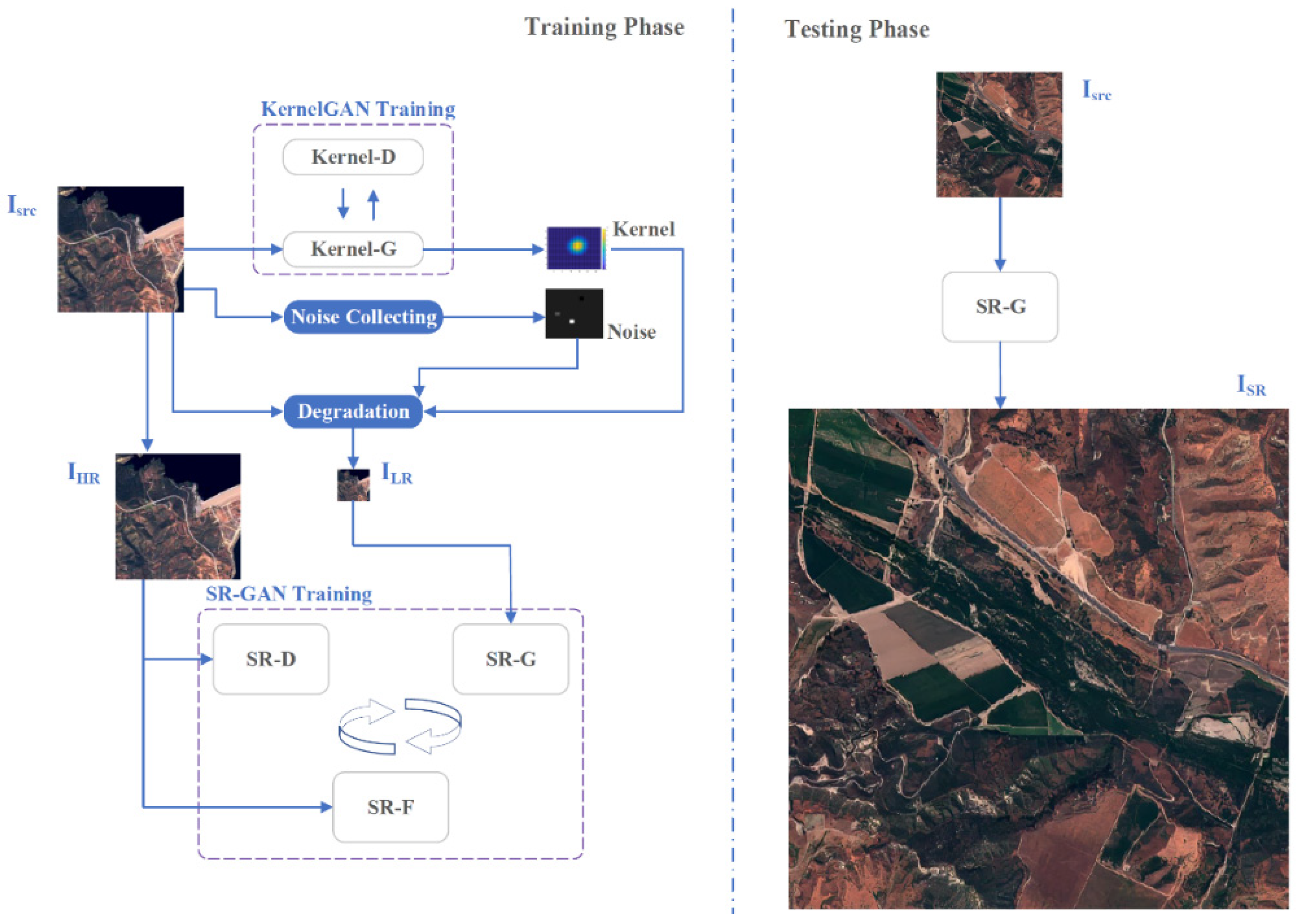
We used TS-SRGAN to generate 2.5 M resolution images I SR from 10 M resolution source images I src of Sentinel-2, in two stages. In the first stage, KernelGAN was used to implement the estimation of the explicit degradation kernel of I src images, and then, along with injecting the degraded noise, the source images I src were degraded to LR images I LR , which we combined with HR images I HR (equivalent to I src ) to construct LR-HR image pairs ( I LR , I HR ). In the second stage, the dataset ( I LR , I HR ) was used to train the super-resolution generative adversarial network (SR-GAN), which consisted of a super-resolution generator (SR-G), a super-resolution discriminator (SR-D), and a super-resolution perceptual-feature extractor (SR-F). TS-SRGAN represents the Sentinel-2 image SR model proposed in this paper, and the structure of TS-SRGAN is shown in Figure 2.

3.2. Degraded Model

Here, we introduce an image degradation model based on the GAN. The natural pairing mapping between HR and LR images can be approximately understood as the degradation relationship between them, and the degradation process can be expressed as follows:
I L R = I S R C * k s s + n
where k s   and n represent the degradation kernel and degraded noise, respectively, and s represents the scaling factor. The quality of the degradation kernel and degraded noise determine the relevance between LR–HR image pairs and natural image pairs, and the accuracy of the extracted mapping features from LR and HR resolution images determines the quality of images generated by SR.

3.2.1. Degradation Kernel Estimation

Here, we first consider the noise-free degradation process, assuming that the noise-free LR image I L R _ c l is the result of the downsampled HR image I S R C , by using the degradation kernel through the scaling factor s :
I L R _ c l = I S R C * k s S
In this paper, KernelGAN is used to estimate the image degradation kernel k s , which is a blind SR degradation kernel estimation model based on Internal-GAN [43] and a completely unsupervised GAN, requiring no extra training data except the image I S R C itself [39]. KernelGAN uses only the images I S R C for training, to learn the distribution of internal pixel patches, with the goal of finding the image-specific degradation kernel and the best degradation kernel to retain the distribution of pixel patches for each scale of the image I S R C . More specifically, the goals are to “generate” downsampled images, and to make the pixel patch distribution of the downsampled images as close to that of the images I S R C as possible. The essence of the model is the extraction of the cross-scale recursive characteristics between LR and HR images through deep learning, and GAN in KernelGAN can be understood as the matching tool for pixel patch distribution. The implementation process of KernelGAN is shown in Figure 3, which illustrates training, using a single input image to learn the distribution of internal pixel patches of the cropped patch. There is a kernel generator (kernel-G) and a kernel discriminator (kernel-D). Both the kernel-G and the kernel-D are fully convolutional, which means that the network is applied to the pixel patch rather than to the whole image. With the given input of images I S R C , the kernel generator will learn to downsample to I L R _ c l , whose goal is to make the discriminator indistinguishable from the input images I S R C at the pixel-patch level.
The objective function of KernelGAN is defined as follows:
G * ( I S R C ) = argmin G m a x D { E x ~ patches ( I S R C ) [ | D ( I S R C ) 1 | + | D ( G ( I S R C ) ) | ] + R }
where G represents the generator and D represents the discriminator. Additionally, R is the regularization term optimized by the degradation kernel k s :
R = α s _ 1 L s _ 1 + α b L b + α sp L sp + α c L c
where L s _ 1 , L b , L sp , L c represent losses, and α s _ 1 , α b , α sp , α c represent constant coefficients. In this study, the constant coefficients were set according to experience as α s _ 1 = 0.5 , α b = 0.5 , α sp = 5 , α c = 1 . The losses are defined as the following equations, respectively:
L s _ 1 = 1 i , j k i , j
where k i , j represents the parameter value of each point of the degradation kernel, and the goal of L s _ 1 is that the sum of k i , j is 1.
L b = i , j k i , j m i , j
The goal of L b is to punish the non-zero value near the boundary, and m i , j is the constant mask of weight, which increases exponentially with the distance from the center of k i , j .
L sp = i , j k i , j 1 / 2
The goal of L sp is the sparsity of k i , j to avoid excess smoothness of the interior kernel.
L c = x 0 , y 0 i , j k i , j ( i , j ) i , j k i , j 2
The goal of L c is to have the center of k i , j in the center of the interior kernel, and x 0 , y 0 represents the indices of the center.
Kernel-G can be regarded as an image downsampling model, which implements linear downsampling mainly through the convolution layer, and the network contains no nonlinear activation unit. A nonlinear generator is not used here because it is possible for the nonlinear generator to generate physically unnecessary solutions for the optimization targets, for example, to generate an image that is not downsampled but contains effective pixel patches. In addition, because the single-layer convolution layer cannot converge accurately, we use the multi-layer structure of linear convolution layers, as in Figure 4.
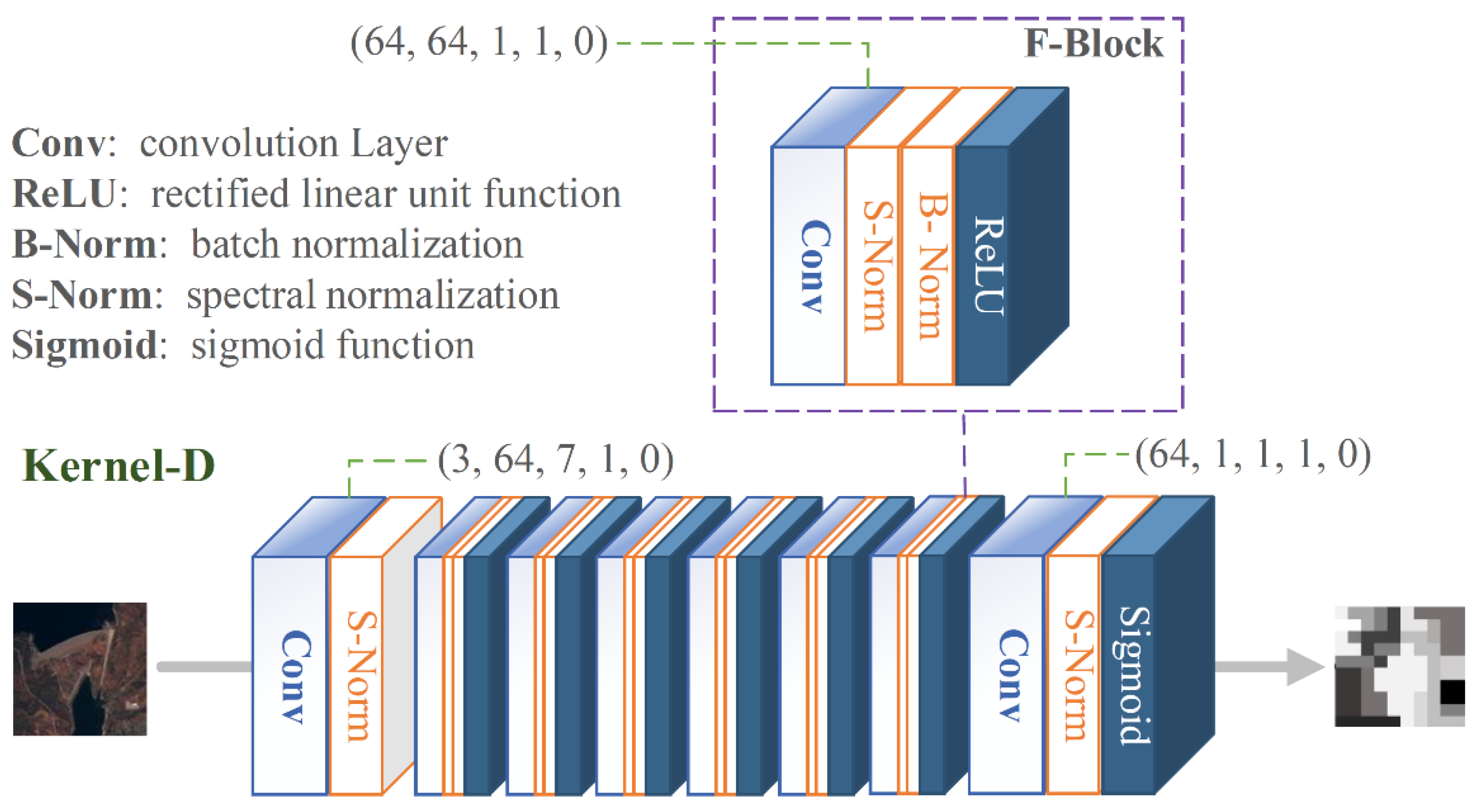
The goal of kernel-D is to learn the distribution of pixel patches in input images I S R C and to distinguish between the real patches and fake patches in the distribution. The real patches are cropped from input images I S R C , and the fake patches are cropped from I L R _ c l generated by kernel-G. We use the fully convolutional pixel-patch discriminator introduced in [44] to learn the pixel patch distribution of every single image, as shown in Figure 5.
The convolution layer used in kernel-D does not perform pooling operations, instead it implicitly acts on each pixel block and finally generates a hot map (D-map), on which each position corresponds to one cropped patch input. The hot map output by kernel-D represents the possibility of each pixel extracting the surrounding pixel patches from the original pixel patch distribution, and it is used to distinguish the real patches from the fake patches. The loss is defined as the pixel-wise mean-square error between the hot map and the label map. The label map refers to all 1 labels of the real patches and all 0 labels of the fake patches.
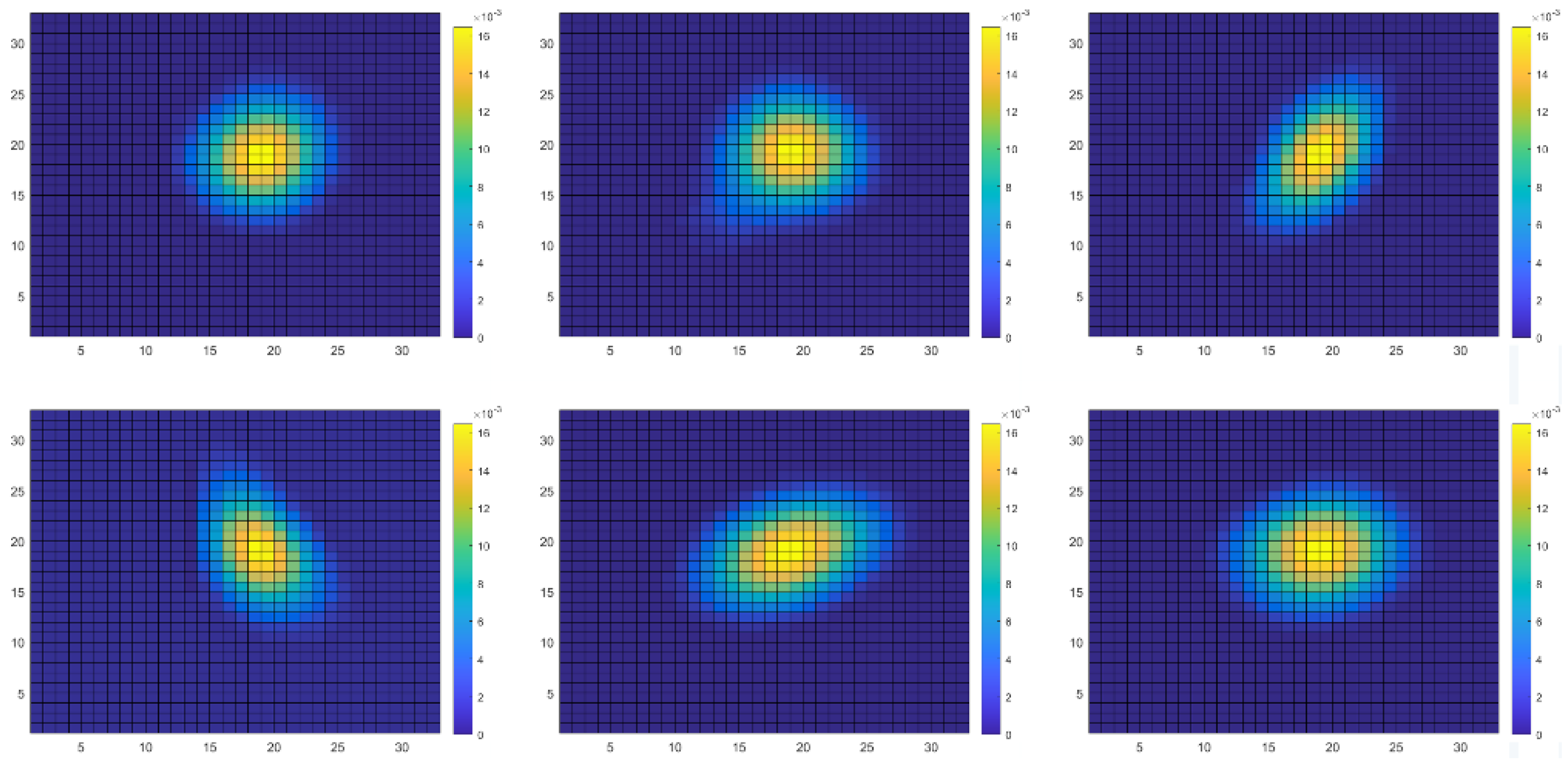
After the training of KernelGAN, we do not focus on the generator network, but convolute the convolution layers of kernel-G with the stride of 1, successively, to extract the explicit degradation kernel. Meanwhile, the training of KernelGAN is based on one single input image, I S R C , which means that each input image trains one degradation kernel, and many degradation kernels generated by the training image set will be randomly selected and used in the subsequent steps. The graphical examples of some degradation kernels are shown in Figure 6.

3.2.2. Generation and Injection of Noise

As opposed to the direct downscaling methods, such as BiCubic, we explicitly inject additional noise into I L R _ c l , so as to keep the noise distributions of I L R and I S R C images as consistent as possible. Due to the large variance of the patches with rocky content [38], and inspired by [40,45], when extracting noise-mapping patches we control the variance within a specific range under the condition:
D n i < σ m a x
where D · represents the variance function, and σ m a x represents the maximum value of the variance. The noise-mapping patches are extracted from images selected from the images of ROI_Src randomly, and a certain number of noise patches are extracted to construct the dataset (ROI_Noi). The noise-mapping patches used for the noise-injection process are randomly selected from ROI_Noi.
To sum up, the process of generating LR images in ROI_LR from the source images in ROI_Src can be expressed as Equation (10), where I and j are randomly selected:
I L R = I S R C * k i s s + n j

3.3. SR-GAN

SR-GAN consists of a super-resolution generator (SR-G), super-resolution discriminator (SR-D) and perceptual-feature extractor (SR-F). SR-G generates a ×4 high-resolution image through learning the characteristics of the training set data. SR-D and SR-F compare the generated image with the ground truth image, respectively. SR-D feeds back pixel-wise loss and adaptive loss to SR-G, and SR-F feeds back perceptual loss to SR-G, realizing SR-D and SR-F’s supervision of SR-G. SR-G was designed on the basis of the ESRGAN [26]. As an ESRGAN discriminator may introduce more artifacts [38], SR-D was designed on the basis of PatchGAN [44]. The perceptual-feature extractor was designed on the basis of VGG-19 [46], so as to introduce the perceptual loss [47], which can strengthen the extraction of low-frequency features and improve the effect of visual perception.
The loss L SR of SR-GAN consists of three parts, including pixel-wise loss L x [26], perceptual loss L p and adversarial loss L a .
L SR = α x L x + α p L p + α a L a
where α x , α p   and   α a are constant coefficients, and the constant coefficients were set according to experience as α x = 0.01 , α p = 1 , α a = 0.005 . The losses L x ,   L p   and   L a are defined as Equations (12), (13) and (16).
L x = E I L R G ( I L R ) I H R 1
Pixel-wise loss L x uses L1 distance to evaluate the pixel-wise content loss between G I L R and I H R .
L p = λ f L f + λ t L t
Perceptual loss L p evaluates the perceived differences in content and style among different images, and consists of feature reconstructing loss L f related to content and style reconstructing loss L t , where λ f   and   λ t denote constant coefficients, and L f and L t   can be expressed as follows:
L f = 1 C j H j W j ϕ j G I L R ϕ j I H R 2 2
L t = 1 C j H j W j h = 1 H j w = 1 W j ϕ j ( G I L R ) h , w , c ϕ j ( G I L R ) h , w , c ϕ j ( I H R ) h , w , c ϕ j ( I H R ) h , w , c F 2
where ϕ j I represents the characteristic diagram obtained at level j of the convolution layer after the image I inputs SR-F, and the shape of the obtained characteristic diagram is C j × H j × W j ( Channel × Height × Width ). · F 2 represents the square Frobenius norm.
L a = n = 1 N D G I L R
Adversarial loss, L a , can enhance the texture details of the image, making the visual effect of the generated image more realistic.
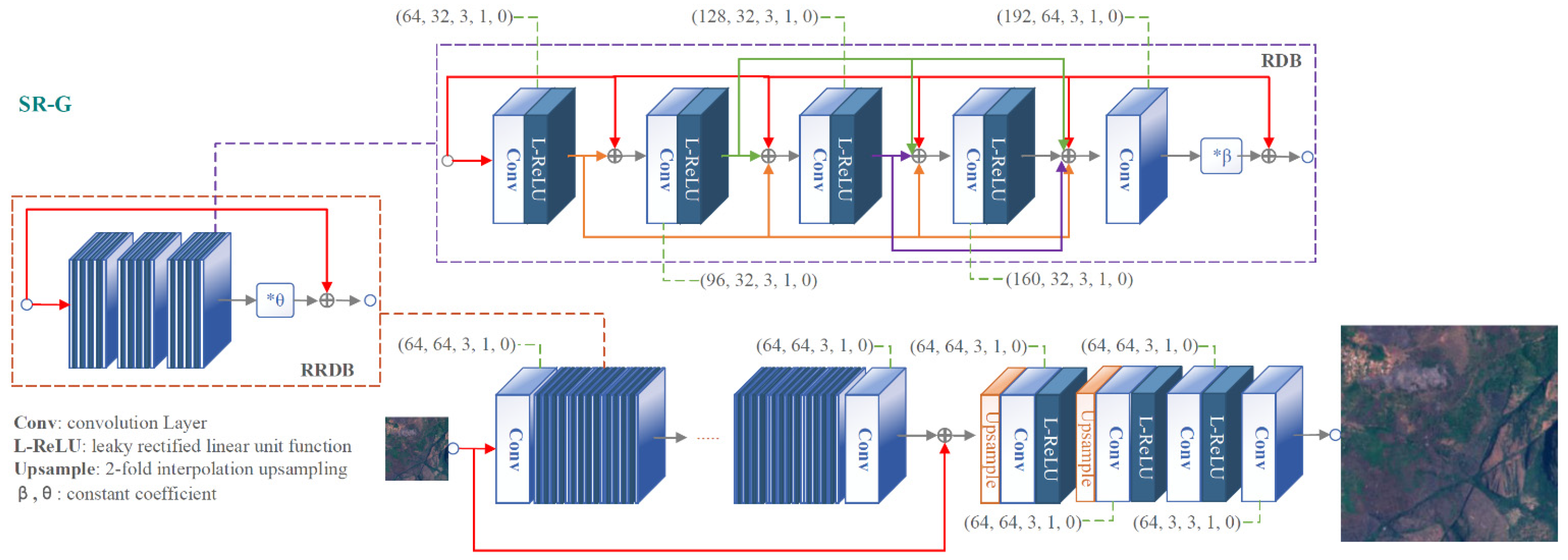
The structure of SR-G is shown in Figure 7. Based on the ESRGAN model, and with the RRDB [39] structure, it was trained in the constructed LR-HR image pairs I L R , I H R , and the resolution of the generated images was magnified ×4.
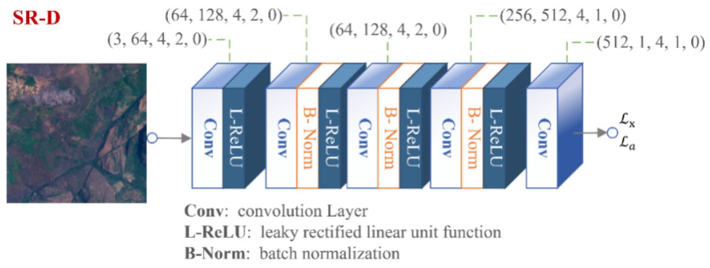
Due to the discriminator in ESRGAN possibly introducing more artifacts, we used the patch discriminator instead of the VGG-128 discriminator in the ESRGAN model, and SR-D was designed based on PatchGAN [44]. In addition, the patch discriminator was used instead of the VGG-128 discriminator, out of consideration for the following aspects: VGG-128 is applied to images with a size of 128 pixels, which makes training on large scales less powerful; VGG-128, when using a fixed fully connected layer, is better at handling global features rather than local features. [34]. For this reason, we use the patch discriminator, which has a fully convolutional structure, and with the receptive field fixed. Each output value of SR-D depends only on the local fixed patches, so that we can optimize the local details. The average value of all local errors is used as the final error, to guarantee global consistency. The structure of SR-D is shown in Figure 8.
Based on the VGG-19 [46] model, this paper introduces the perceptual-feature extractor to extract the perceptual loss L p , that is, to extract the inactive features in VGG-19. The perceptual loss can enhance the low-frequency features of the images and make the images generated by the generator look more realistic. The structure of the perceptual-feature extractor is shown in Figure 9.

4. Experiments and Results

Training Details

The proposed model, TS-SRGAN, and other models, such as EDSR8-RGB, RCAN, RS-ESRGAN and RealSR, were run in a Pytorch environment, using the modules provided by the “sefibk/KernelGAN” project [39], “xinntao/BasicSR” project [48] and “Tencent/Real-SR” project [38] in the Github library. BiCubic can be obtained directly, using Matlab functions to perform interpolation operations.
TS-SRGAN first generates an LR–HR image pair dataset (ROI_Tr) based on a training dataset (ROI_Src) for training and testing. We randomly selected 2134 images from 40,099 images of ROI_Src to generate a degraded kernel dataset (ROI_Ker) through KernelGAN training, one by one, namely, k i s ROI _ Ker , i 1 , 2 2134 ; and then randomly selected 4972 images from 40,099 images of ROI_Src to extract noise patches, one by one, to form a noise patch dataset (ROI_Noi), namely, n j ROI _ Noi , j 1 , 2 4972 ; finally, we used the degradation kernel and injected noise to perform degrading operations on the images in ROI_Src, one by one. In the processing of each image, the degradation kernel and injected noise were randomly selected from ROI_Ker and ROI_Noi.
The network structural parameters of kernel-G and the kernel-D and the constant coefficients of losses of KernelGAN have been mentioned above, so we will not repeat them here. In the training phase, both the generator and the discriminator used an ADAM optimizer with the parameters β 1 = 0.5 ,     β 2 = 0.999 ; the learning rates of kernel-G and kernel-D were both set to 0.0002, decrementing by ×0.1 every 750 iterations, and the network was iteratively trained for 3000 epochs.
SR-G used the “RRDBNet” model in the “BasicSR” project, and SR-D used the “NlayerDiscriminator” model in the “Real-SR” project. The networks’ structural parameters and the constant coefficients of losses have been mentioned above; therefore, we will not repeat them here. The image was magnified by 4 times, and during the training phase both the generator and the discriminator used the ADAM optimizer with the parameters β 1 = 0.9 ,   β 2 = 0.999 ; the learning rates of SR-G and SR-D were both set to 0.0001, and the network was iteratively trained for 60,000 epochs.
Some convolutional layers were used in TS-SRGAN, and these convolutional layers play a vital role. After many tests, it became known that the parameters of the convolutional layer in the network needed to be set as in Table 1, to achieve the ×4 resolution images TS-SRGAN and obtain the image quality we wanted.
The EDSR8-RGB, RCAN, RS-ESRGAN and RealSR models implemented training and testing under the frameworks of BasicSR [48] and Real-SR [38], with the parameter-setting schemes which have been proven to achieve the best results in references [21,32,33]. The parameters used in the implementations are detailed in Table 2.
As the source images used are already the highest resolution (10 m) images of Sentinel-2, there are no real ground truth images (2.5 M resolution) that can be compared with the generated images in reality, and some image-quality assessment metrics commonly used, such as, PSNR and SSIM, are not applicable in this scenario. Therefore, we adopted non-reference image quality assessment (NR-IQA) metrics, including NIQE [49], BRISQUE [50] and PIQE [51]. The evaluation values of NIQE, BRISQUE and PIQE can be calculated by the corresponding functions NIQE, BRISQE and PIQE in Matlab; the output results of the three functions are all within the range of [0, 100], where the lower the score, the higher the perceived effect.
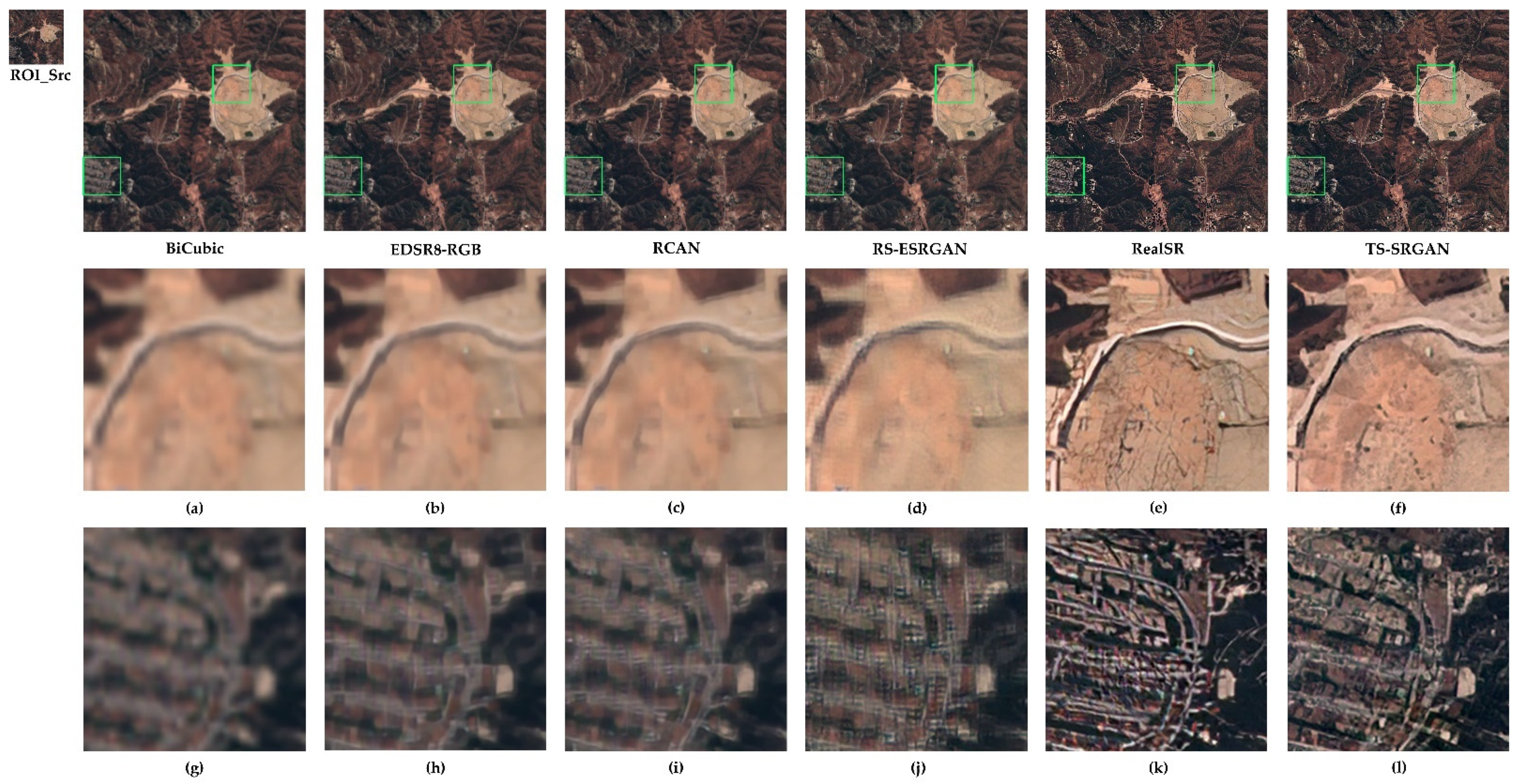
We randomly selected one sub-dataset, “ROIs1158_spring_106,” in ROIs1158, as the testing dataset (ROI_Te) containing 784 images. The remote-sensing images in ROI_Te were collected from the ground areas, as shown in Figure 10. In the figure we marked eight regions with strong geographic features, and the ×4 generated images of these regions are shown subsequently, to visually compare the differences among those models.
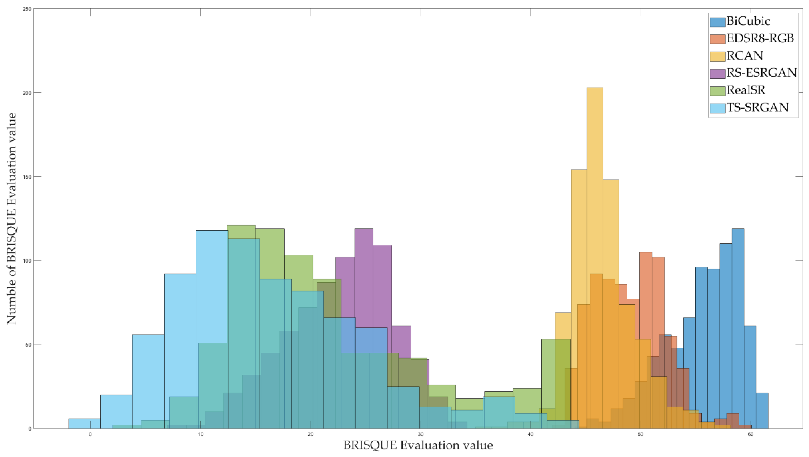
We used the BiCubic, EDSR8-RGB, RCAN, RS-ESRGAN and TS-SRGAN models to process 784 images in ROI_Te to generate ×4 HR images, and used Matlab to calculate the evaluation values of NIQE, BRISQUE and PIQE, one by one, for the images. The histograms were drawn according to the distributions of evaluation metric values, as shown in Figure 11, Figure 12 and Figure 13, and the mean and extreme values based on the evaluation values are provided in Table 3. The histograms and table show that the TS-SRGAN model is superior to the other models in a variety of NR-IQA metrics.
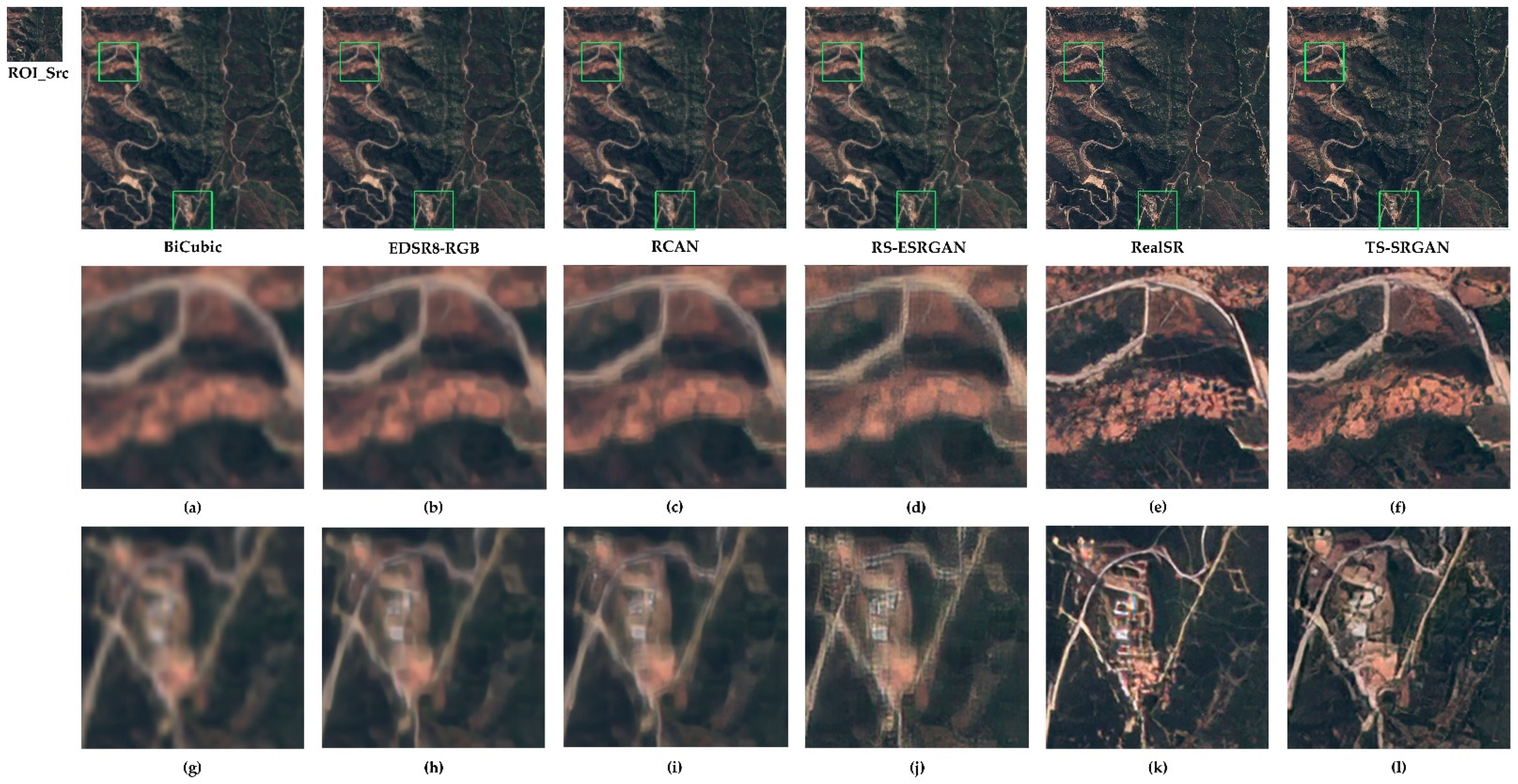
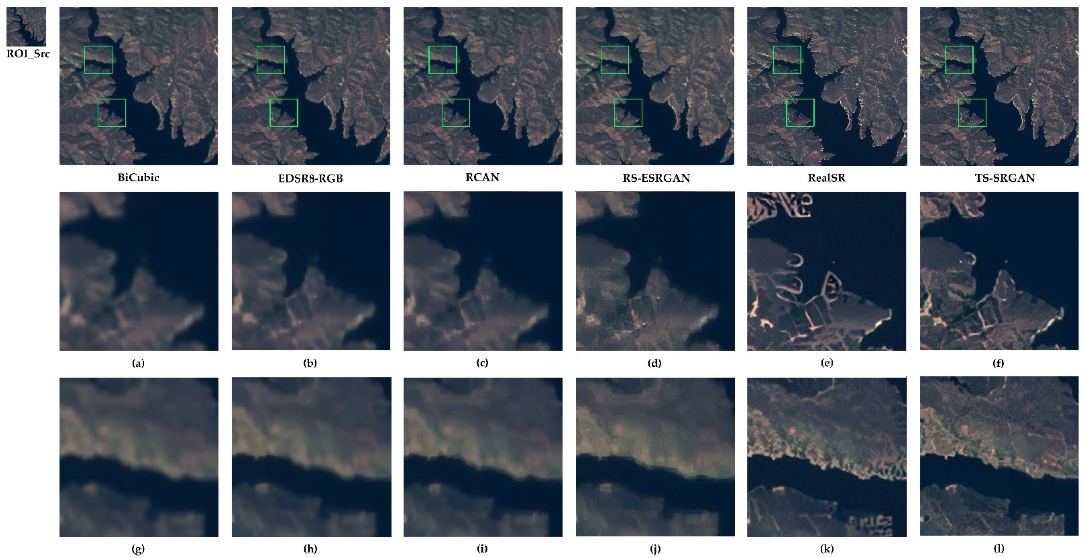
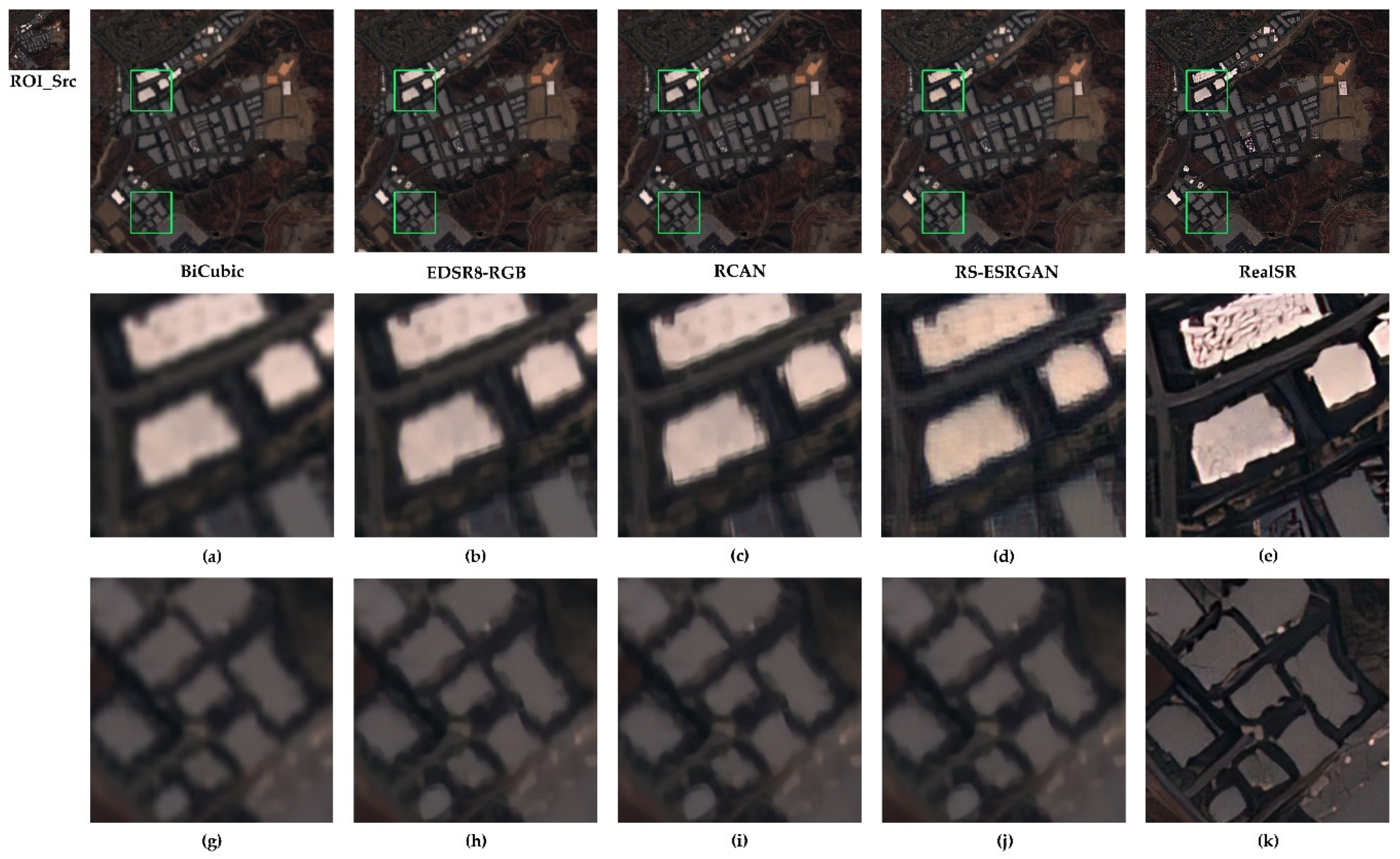
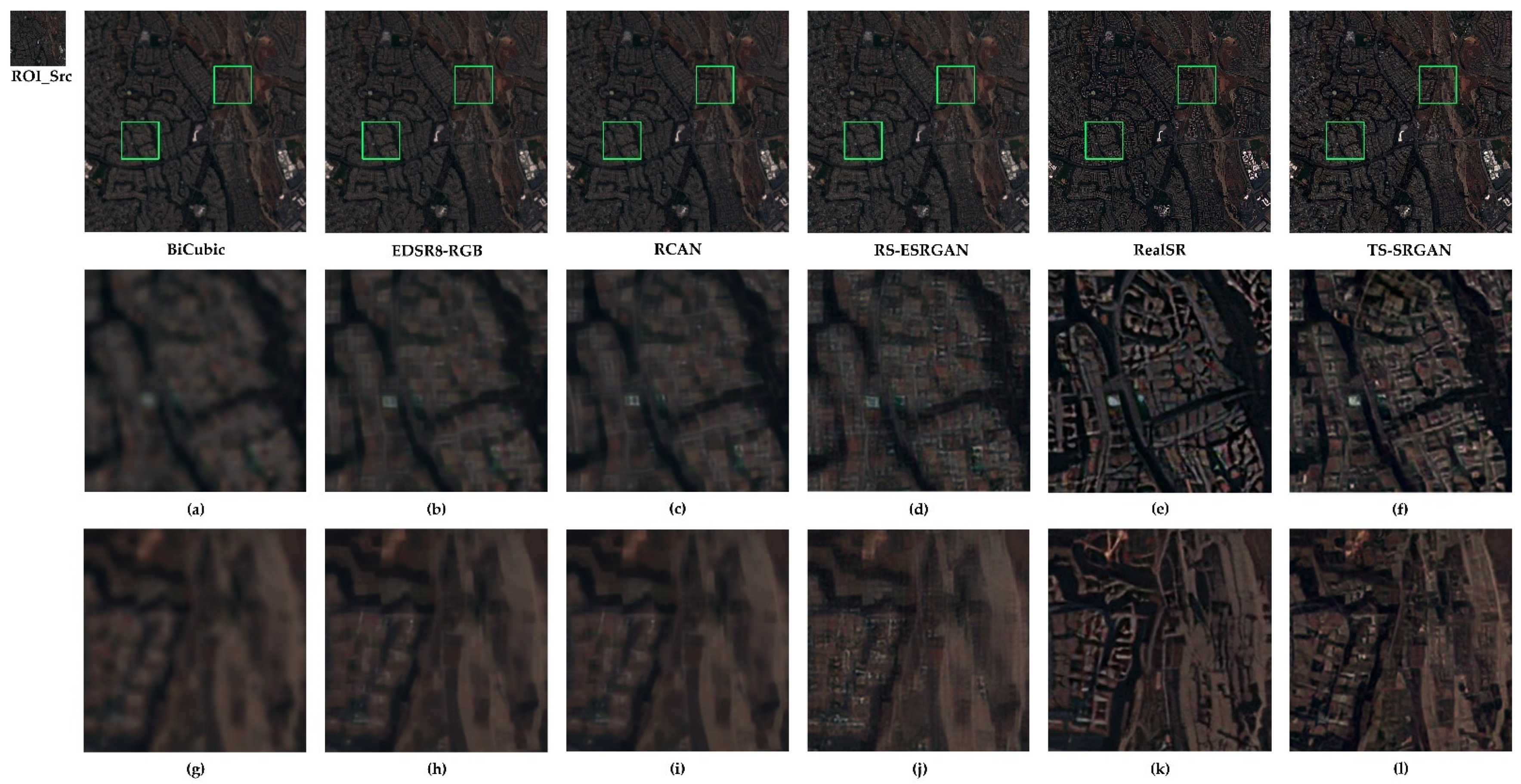
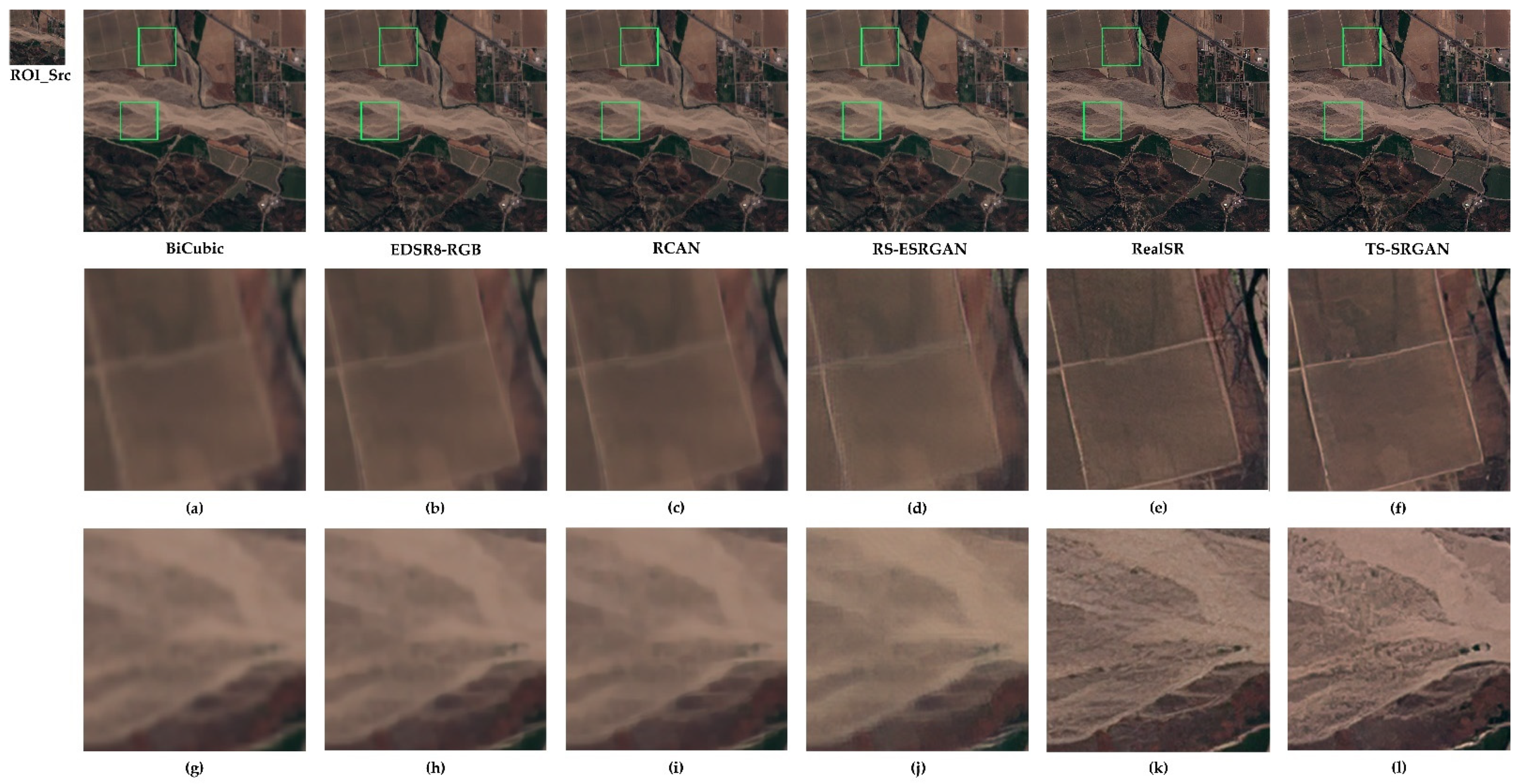
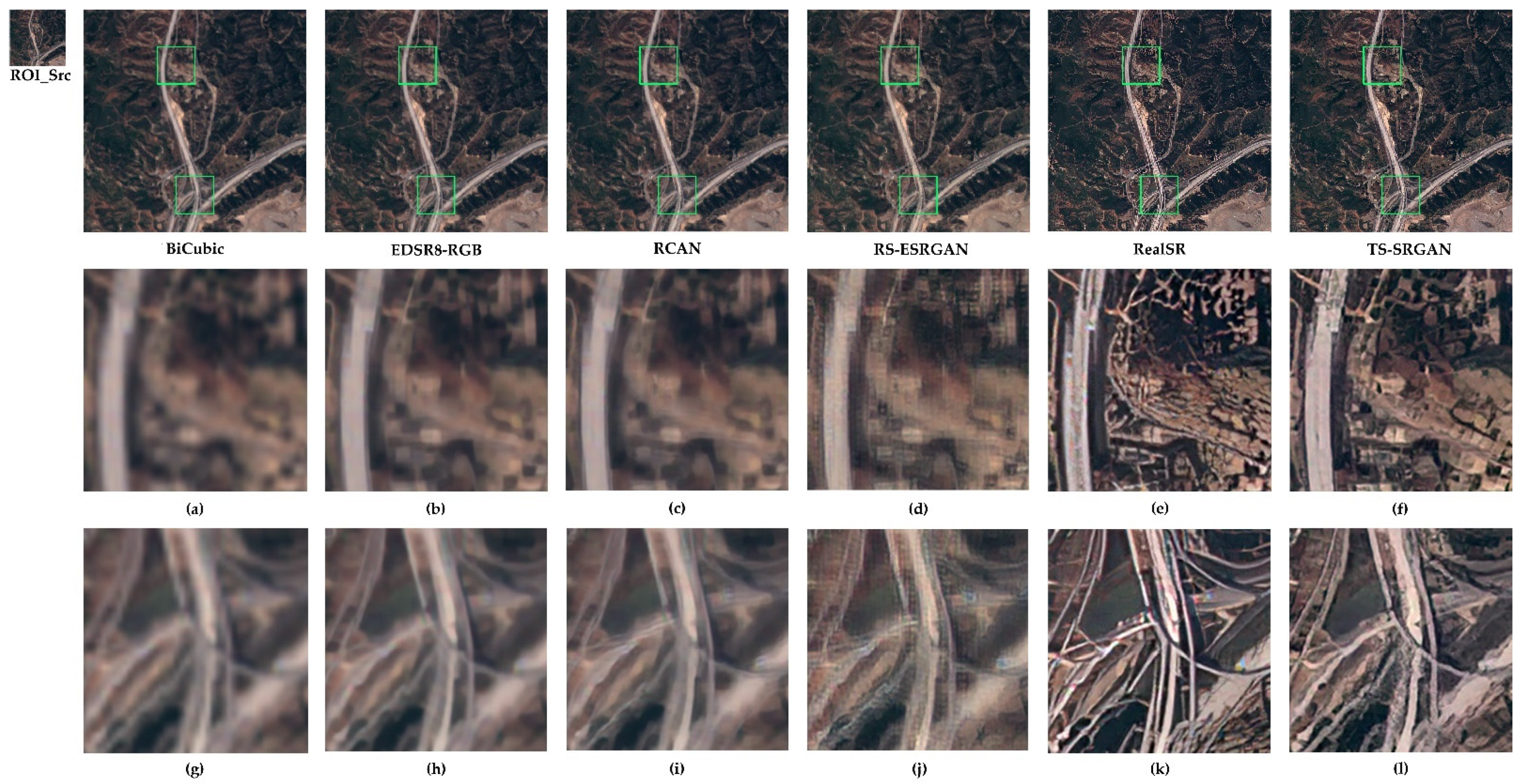
Figure 14, Figure 15, Figure 16, Figure 17, Figure 18, Figure 19, Figure 20 and Figure 21 show the generated images of eight regions with strong geographic features selected in “ROIs1158_spring_106” to visually compare the differences among the models. Through the comparison of the images of various terrains in Figure 14, Figure 15, Figure 16, Figure 17, Figure 18, Figure 19, Figure 20 and Figure 21, it can be clearly seen that the images processed by the traditional BiCubic method are the most bleary and smooth, due to the inherent deficiencies of the interpolation algorithm. The EDSR8-RGB, RCAN and RS-ESRGAN models cannot correctly distinguish the noise with sharp edges, resulting in blurred results, and even indistinguishable houses and roads. As shown in the TS-SRGAN results, the dividing lines among the objects and backgrounds, such as roads, bridges and houses, are much clearer, which indicates that the noise we estimated was closer to the real noise. By using different combinations of degradation (e.g., blur and noise), TS-SRGAN has obtained LR images sharing the same domain with real images, which can avoid the generated LR images being too smooth and fuzzy. Using the super-resolution network trained by the domain-consistent data, TS-SRGAN generates HR images with clearer boundaries and better perception. Compared with the EDSR8-RGB, RCAN and RS-ESRGAN models, the TS-SRGAN’s results are clearer, and have no ambiguity.

5. Conclusions

In this paper, based on the latest and most widely recognized GAN technologies, including KernelGAN, ESRGAN, PatchGAN, etc., we introduced the degradation kernel estimation and noise injection to perform SR for Sentinel-2 satellites’ remote-sensing images, and improved the highest-resolution images from 10 M to 2.5 M resolution. Through the combination of the degradation kernel and injected noise, we obtained LR images in the same domain with real images, and obtained the near-natural LR–HR image pairs. On the basis of near-natural LR–HR image pairs, we used a GAN, combined with an ESRGAN-type generator, a PatchGAN-type discriminator and a VGG-19-type feature extractor, used the perceptual loss, and focused on the visual characteristics of the images, so that our results have clearer details and better perceptual effects. Compared with the SR models of Sentinel-2, such as EDSR8-RGB, RCAN, RS-ESRGAN and RealSR, the main difference in our model lies in the construction of LR–HR image pairs for the training datasets. In the scene of training with natural LR–HR image pairs, there was no significant difference in the effect for SR images obtained with those models; however, in the scene with only LR images and no HR prior information, compared with RCAN, which constructs the image pairs through BiCubic and EDSR8-RGB and RS-ESRGAN, which use WorldView satellite HR images to construct the image pairs, TS-SRGAN has obvious advantages in the quantitative comparison of the non-reference image quality assessment and the intuitive visual effects.

Author Contributions

Conceptualization, Y.L. and S.W.; methodology, Y.L.; software, Y.L. and Y.W.; validation, Y.L. and, Y.W.; formal analysis, Y.L.; resources, Y.L., S.W. and B.L.; writing—original draft preparation, Y.L., Y.W. and B.L.; writing—review and editing, B.L.; project administration, Y.L.; funding acquisition, Y.L. and S.W. All authors have read and agreed to the published version of the manuscript.

Funding

This research was funded by the National Natural Science Foundation of China (Grant No. 61871147); Natural Science Foundation of Guangdong Province, China (Grant No. 2018A030313346); the General University Key Field Special Project of Guangdong Province, China (Grant No. 2020ZDZX3078); the General University Key Field Special Project of Guangdong Province, China (Grant No. 2022ZDZX1035); the Research Fund Program of Guangdong Key Laboratory of Aerospace Communication and Networking Technology (Grant No. 2018B030322004).

Data Availability Statement

The ×4 images by models TS-SRGAN, BiCubic, EDSR8-RGB, RCAN, RS-ESRGAN and RealSR are available online at Baidu Wangpan (code: mbah). The trained models of TS-SRGAN, EDSR8-RGB, RCAN, RS-ESRGAN and RealSR are available online at Baidu Wangpan (code: 5xj6). Additionally, all the codes generated or used during the study are available online at github/TS-RSGAN.

Acknowledgments

This work has a preprint version [52]. This version has not been peer-reviewed.

Conflicts of Interest

The authors declare no conflict of interest. The funders had no role in the design of the study, in the collection, analyses, or interpretation of data, in the writing of the manuscript, or in the decision to publish the results.

References

  1. Verbyla, D.L. Satellite Remote Sensing of Natural Resources; CRC Press: Boca Raton, FL, USA, 1995. [Google Scholar]
  2. Ye, B.; Tian, S.; Ge, J.; Sun, Y. Assessment of WorldView-3 data for lithological mapping. Remote Sens. 2017, 9, 1132. [Google Scholar] [CrossRef]
  3. Williams, D.L.; Goward, S.; Arvidson, T. Landsat. Photogramm. Eng. Remote Sens. 2006, 72, 1171–1178. [Google Scholar] [CrossRef]
  4. Sentinel, E. User Handbook. ESA Standard Document. 2015, Volume 64. Available online: https://earth.esa.int/documents/247904/685211/Sentinel-2_User_Handbook (accessed on 24 July 2015).
  5. Gargiulo, M.; Mazza, A.; Gaetano, R.; Ruello, G.; Scarpa, G. Fast Super-Resolution of 20 m Sentinel-2 Bands Using Convolutional Neural Networks. Remote Sens. 2019, 11, 2635. [Google Scholar] [CrossRef] [Green Version]
  6. Lu, J.; He, T.; Song, D.-X.; Wang, C.-Q. Land surface phenology retrieval through spectral and angular harmonization of landsat-8, sentinel-2 and gaofen-1 data. Remote Sens. 2022, 14, 1296. [Google Scholar] [CrossRef]
  7. Yang, X.; Zhao, S.; Qin, X.; Zhao, N.; Liang, L. Mapping of urban surface water bodies from Sentinel-2 MSI imagery at 10 m resolution via NDWI-based image sharpening. Remote Sens. 2017, 9, 596. [Google Scholar] [CrossRef] [Green Version]
  8. Gasmi, A.; Gomez, C.; Chehbouni, A.; Dhiba, D.; Elfil, H. Satellite multi-sensor data fusion for soil clay mapping based on the spectral index and spectral bands approaches. Remote Sens. 2022, 14, 1103. [Google Scholar] [CrossRef]
  9. Li, H.; Shi, D.; Wang, W.; Liao, D.; Gadekallu, T.R.; Yu, K. Secure routing for LEO satellite network survivability. Comput. Netw. 2022, 211, 109011. [Google Scholar] [CrossRef]
  10. Li, H.; Zhao, L.; Sun, L.; Li, X.; Wang, J.; Han, Y.; Liang, S.; Chen, J. Capability of Phenology-Based Sentinel-2 Composites for Rubber Plantation Mapping in a Large Area with Complex Vegetation Landscapes. Remote Sens. 2022, 14, 5338. [Google Scholar] [CrossRef]
  11. Wang, J.; Huang, B.; Zhang, H.K.; Ma, P. Sentinel-2A image fusion using a machine learning approach. IEEE Trans. Geosci. Remote Sens. 2019, 57, 9589–9601. [Google Scholar] [CrossRef]
  12. Rumora, L.; Gašparović, M.; Miler, M.; Medak, D. Quality assessment of fusing Sentinel-2 and WorldView-4 imagery on Sentinel-2 spectral band values: A case study of Zagreb, Croatia. Int. J. Image Data Fusion 2020, 11, 77–96. [Google Scholar] [CrossRef]
  13. Yang, J.; Wright, J.; Huang, T.S.; Ma, Y. Image super-resolution via sparse representation. IEEE Trans. Image Process. 2010, 19, 2861–2873. [Google Scholar] [CrossRef] [PubMed]
  14. Gou, S.; Liu, S.; Yang, S.; Jiao, L. Remote sensing image super-resolution reconstruction based on nonlocal pairwise dictionaries and double regularization. IEEE J. Sel. Top. Appl. Earth Obs. Remote Sens. 2014, 7, 4784–4792. [Google Scholar] [CrossRef]
  15. Pan, Z.; Yu, J.; Huang, H.; Hu, S.; Zhang, A.; Ma, H.; Sun, W. Super-resolution based on compressive sensing and structural self-similarity for remote sensing images. IEEE Trans. Geosci. Remote Sens. 2013, 51, 4864–4876. [Google Scholar] [CrossRef]
  16. Zhang, Y.; Du, Y.; Ling, F.; Fang, S.; Li, X. Example-based super-resolution land cover mapping using support vector regression. IEEE J. Sel. Top. Appl. Earth Obs. Remote Sens. 2014, 7, 1271–1283. [Google Scholar] [CrossRef]
  17. Li, J.; Yuan, Q.; Shen, H.; Meng, X.; Zhang, L. Hyperspectral image super-resolution by spectral mixture analysis and spatial–spectral group sparsity. IEEE Geosci. Remote Sens. Lett. 2016, 13, 1250–1254. [Google Scholar] [CrossRef]
  18. Wang, Z.; Chen, J.; Hoi, S.C.H. Deep learning for image super-resolution: A survey. IEEE Trans. Pattern Anal. Mach. Intell. 2021, 43, 3365–3387. [Google Scholar] [CrossRef] [PubMed] [Green Version]
  19. Dong, C.; Loy, C.C.; He, K.; Tang, X. Learning a deep convolutional network for image super-resolution. In Proceedings of the Computer Vision-ECCV 2014, Zurich, Switzerland, 6–12 September 2014; Fleet, D., Pajdla, T., Schiele, B., Tuytelaars, T., Eds.; Springer: Cham, Switzerland, 2014; pp. 184–199. [Google Scholar]
  20. Kim, J.; Lee, J.K.; Lee, K.M. Accurate image super-resolution using very deep convolutional networks. In Proceedings of the IEEE Conference on Computer Vision and Pattern Recognition, Las Vegas, NV, USA, 26 June–1 July 2016; pp. 1646–1654. [Google Scholar]
  21. Zhang, Y.; Li, K.; Li, K.; Wang, L.; Zhong, B.; Fu, Y. Image super-resolution using very deep residual channel attention networks. In Proceedings of the European Conference on Computer Vision (ECCV), Munich, Germany, 8–14 September 2018; pp. 286–301. [Google Scholar]
  22. Tai, Y.; Yang, J.; Liu, X. Image super-resolution via deep recursive residual network. In Proceedings of the IEEE Conference on Computer Vision and Pattern Recognition, Honolulu, HI, USA, 21–26 July 2017; pp. 3147–3155. [Google Scholar]
  23. Hu, J.; Shen, L.; Sun, G. Squeeze-and-excitation networks. In Proceedings of the IEEE Conference on Computer Vision and Pattern Recognition, Salt Lake City, UT, USA, 18–23 June 2018; pp. 7132–7141. [Google Scholar]
  24. Goodfellow, I.; Pouget-Abadie, J.; Mirza, M.; Xu, B.; Warde-Farley, D.; Ozair, S.; Courville, A.; Bengio, Y. Generative adversarial networks. Commun. ACM 2014, 63, 139–144. [Google Scholar] [CrossRef]
  25. Ledig, C.; Theis, L.; Huszar, F.; Caballero, J.; Cunningham, A.; Acosta, A.; Aitken, A.; Tejani, A.; Totz, J.; Wang, Z.; et al. Photo-realistic single image super-resolution using a generative adversarial network. In Proceedings of the IEEE Conference on Computer Vision and Pattern Recognition, Honolulu, HI, USA, 21–26 July 2017; pp. 4681–4690. [Google Scholar]
  26. Wang, X.; Yu, K.; Wu, S.; Gu, J.; Liu, Y.; Dong, C.; Qiao, Y.; Loy, C.C. Esrgan: Enhanced super-resolution generative adversarial networks. In Proceedings of the European Conference on Computer Vision (ECCV) Workshops, Munich, Germany, 8–14 September 2018. [Google Scholar]
  27. Ma, W.; Pan, Z.; Guo, J.; Lei, B. Super-resolution of remote sensing images based on transferred generative adversarial network. In Proceedings of the IGARSS 2018—2018 IEEE International Geoscience and Remote Sensing Symposium, Valencia, Spain, 22–27 July 2018; pp. 1148–1151. [Google Scholar]
  28. Haut, J.M.; Paoletti, M.E.; Fernández-Beltran, R.; Plaza, J.; Plaza, A.; Li, J. Remote sensing single-image superresolution based on a deep compendium model. IEEE Geosci. Remote Sens. Lett. 2019, 16, 1432–1436. [Google Scholar] [CrossRef]
  29. Haut, J.M.; Fernandez-Beltran, R.; Paoletti, M.E.; Plaza, J.; Plaza, A. Remote sensing image superresolution using deep residual channel attention. IEEE Trans. Geosci. Remote Sens. 2019, 57, 9277–9289. [Google Scholar] [CrossRef]
  30. Lei, S.; Shi, Z.; Zou, Z. Super-resolution for remote sensing images via local–global combined network. IEEE Geosci. Remote Sens. Lett. 2017, 14, 1243–1247. [Google Scholar] [CrossRef]
  31. Gong, Y.; Liao, P.; Zhang, X.; Zhang, L.; Chen, G.; Zhu, K.; Tan, X.; Lv, Z. Enlighten-GAN for Super Resolution Reconstruction in Mid-Resolution Remote Sensing Images. Remote Sens. 2021, 13, 1104. [Google Scholar] [CrossRef]
  32. Galar, M.; Sesma, R.; Ayala, C.; Albizua, L.; Aranda, C. Super-Resolution of Sentinel-2 Images Using Convolutional Neural Networks and Real Ground Truth Data. Remote Sens. 2020, 12, 2941. [Google Scholar] [CrossRef]
  33. Salgueiro Romero, L.; Marcello, J.; Vilaplana, V. Super-Resolution of Sentinel-2 Imagery Using Generative Adversarial Networks. Remote Sens. 2020, 12, 2424. [Google Scholar] [CrossRef]
  34. Zhang, W.; Liu, Y.; Dong, C.; Qiao, Y. Ranksrgan: Generative adversarial networks with ranker for image super-resolution. In Proceedings of the IEEE/CVF International Conference on Computer Vision, Seoul, Korea, 27 October–2 November 2019; pp. 3096–3105. [Google Scholar]
  35. Jiang, K.; Wang, Z.; Yi, P.; Wang, G.; Lu, T.; Jiang, J. Edge-enhanced GAN for remote sensing image superresolution. IEEE Trans. Geosci. Remote Sens. 2019, 57, 5799–5812. [Google Scholar] [CrossRef]
  36. Wang, Z.; Jiang, K.; Yi, P.; Han, Z.; He, Z. Ultra-dense GAN for satellite imagery super-resolution. Neurocomputing 2020, 398, 328–337. [Google Scholar] [CrossRef]
  37. Zhu, X.; Zhang, L.; Zhang, L.; Liu, X.; Shen, Y.; Zhao, S. GAN-based image super-resolution with a novel quality loss. Math. Probl. Eng. 2020, 2020, 5217429. [Google Scholar] [CrossRef]
  38. Ji, X.; Cao, Y.; Tai, Y.; Wang, C.; Li, J.; Huang, F. Real-world super-resolution via kernel estimation and noise injection. In Proceedings of the IEEE/CVF Conference on Computer Vision and Pattern Recognition Workshops, Seattle, WA, USA, 13–19 June 2020; pp. 466–467. [Google Scholar]
  39. Bell-Kligler, S.; Shocher, A.; Irani, M. Blind super-resolution kernel estimation using an internal-gan. Adv. Neural Inf. Process. Syst. 2019, 32, 1–10. [Google Scholar]
  40. Chen, J.; Chen, J.; Chao, H.; Yang, M. Image blind denoising with generative adversarial network based noise modeling. In Proceedings of the IEEE Conference on Computer Vision and Pattern Recognition, Salt Lake City, UT, USA, 18–23 June 2018; pp. 3155–3164. [Google Scholar]
  41. Schmitt, M.; Hughes, L.H.; Qiu, C.; Zhu, X.X. SEN12MS-A curated dataset of georeferenced multi-spectral sentinel-1/2 imagery for deep learning and data fusion. arXiv 2019, arXiv:1906.07789. [Google Scholar] [CrossRef] [Green Version]
  42. Wang, H.-p.; Zhou, L.-l; Zhang, J. Region-based Bicubic image interpolation algorithm. Comput. Eng. 2010, 19, 216–218. [Google Scholar]
  43. Shocher, A.; Bagon, S.; Isola, P.; Irani, M. Ingan: Capturing and remapping the “dna” of a natural image. In Proceedings of the IEEE/CVF International Conference on Computer Vision, Seoul, Korea, 27 October–2 November 2019. [Google Scholar]
  44. Isola, P.; Zhu, J.-Y.; Zhou, T.; Efros, A.A. Image-to-image translation with conditional adversarial networks. In Proceedings of the IEEE Conference on Computer Vision and Pattern Recognition, Honolulu, HI, USA, 21–26 July 2017; pp. 1125–1134. [Google Scholar]
  45. Zhou, R.; Susstrunk, S. Kernel modeling super-resolution on real low-resolution images. In Proceedings of the IEEE/CVF International Conference on Computer Vision, Seoul, Korea, 27 October–2 November 2019; pp. 2433–2443. [Google Scholar]
  46. Simonyan, K.; Zisserman, A. Very deep convolutional networks for large-scale image recognition. arXiv 2014, arXiv:1409.1556. [Google Scholar]
  47. Johnson, J.; Alahi, A.; Fei-Fei, L. Perceptual losses for real-time style transfer and super-resolution. In Proceedings of the Computer Vision-ECCV 2014, Zurich, Switzerland, 6–12 September 2014; Leibe, B., Matas, J., Sebe, N., Welling, M., Eds.; Springer: Cham, Switzerland, 2016; pp. 694–711. [Google Scholar]
  48. Wang, X.; Yu, K.; Chan, K.C.K.; Dong, C.; Loy, C.C. BasicSR. Available online: https://github.com/xinntao/BasicSR (accessed on 19 August 2020).
  49. Mittal, A.; Soundararajan, R.; Bovik, A.C. Making a “completely blind” image quality analyzer. IEEE Signal Process. Lett. 2012, 20, 209–212. [Google Scholar] [CrossRef]
  50. Mittal, A.; Moorthy, A.K.; Bovik, A.C. No-reference image quality assessment in the spatial domain. IEEE Trans. Image Process. 2012, 21, 4695–4708. [Google Scholar] [CrossRef] [PubMed]
  51. Venkatanath, N.; Praneeth, D.; Bh, M.C.; Channappayya, S.S.; Medasani, S.S. Blind image quality evaluation using perception based features. In Proceedings of the 2015 Twenty First National Conference on Communications (NCC), Mumbai, India, 27 February–1 March 2015; pp. 1–6. [Google Scholar]
  52. Li, Y.; Li, B. Super-Resolution of Sentinel-2 Images at 10m Resolution without Reference Images. Preprints 2021, 2021040556. [Google Scholar] [CrossRef]
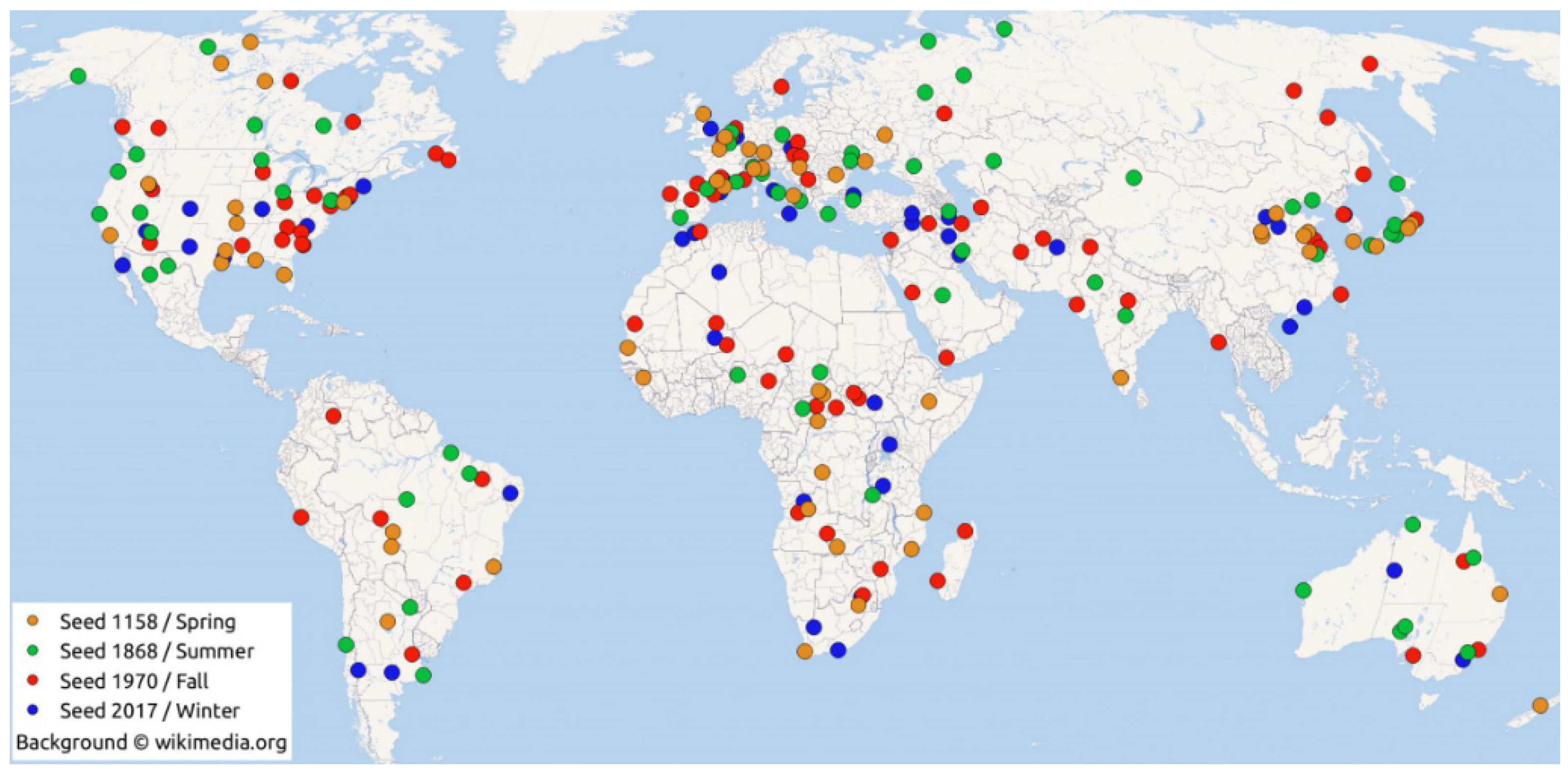
Figure 1. Distribution of regions of interest corresponding to four random seeds.
Electronics 11 03474 g001
Figure 2. Structure of TS-SRGAN on Sentinel-2 remote-sensing images.
Electronics 11 03474 g002
Figure 3. Structure of KernelGAN.
Electronics 11 03474 g003
Figure 4. Network structure of the kernel generator consisting of a multi-layer linear convolution layer.
Electronics 11 03474 g004
Figure 5. Discriminator network structure consisting of a multi-layer non-pooled convolution layer.
Electronics 11 03474 g005
Figure 6. Graphical example of a degradation kernel extracted after KernelGAN training.
Electronics 11 03474 g006
Figure 7. Structure of the super-resolution generator (SR-G).
Electronics 11 03474 g007
Figure 8. Structure of the super-resolution discriminator (SR-D).
Electronics 11 03474 g008
Figure 9. Structure of the perceptual-feature extractor (SR-F).
Electronics 11 03474 g009
Figure 10. Ground map corresponding to sub-dataset “Rois1158_spring_106.”.
Electronics 11 03474 g010
Figure 11. Distribution of evaluation values of NR-IQA metric NIQE.
Electronics 11 03474 g011
Figure 12. Distribution of evaluation values of NR-IQA metric BRISQUE.
Electronics 11 03474 g012
Figure 13. Distribution of evaluation values of NR-IQA metric PIQE.
Electronics 11 03474 g013
Figure 14. Comparison of visual effects of the generated images of the region containing mountain-road terrain. NR-IQA of images (NIQE, BRISQUE, PIQE): BiCubic (6.28, 54.73, 91.87), EDSR8-RGB (5.85, 50.25, 86.05), RCAN (4.64, 47.69, 62.20), RS-ESRGAN (3.31, 22.16, 8.42), RealSR (3.16, 15.75, 8.52), TS-SRGAN (2.43, 7.36, 7.48). The subfigures (al) in the figure represent an enlarged view of the local details in the green boxes in the generated image.
Electronics 11 03474 g014
Figure 15. Comparison of visual effects of the generated images of the region with hilly terrain. NR-IQA of images (NIQE, BRISQUE, PIQE): BiCubic (6.35, 58.38, 92.36), EDSR8-RGB (5.88, 48.02, 81.31), RCAN (4.62, 46.94, 52.83), RS-ESRGAN (3.99, 27.62, 7.61), RealSR (2.83, 13.25, 7.84), TS-SRGAN (2.74, 3.83, 15.57). The subfigures (al) in the figure represent an enlarged view of the local details in the green boxes in the generated image.
Electronics 11 03474 g015
Figure 16. Comparison of visual effects of the generated images of the region containing surface water terrain. NR-IQA of images (NIQE, BRISQUE, PIQE): BiCubic (6.54, 55.52, 100.00), EDSR8-RGB (5.29, 46.00, 76.57), RCAN (4.67, 46.28, 74.49), RS-ESRGAN (3.53, 27.75, 12.08), RealSR (2.56, 13.68, 9.84), TS-SRGAN (2.42, 13.97, 10.03). The subfigures (al) in the figure represent an enlarged view of the local details in the green boxes in the generated image.
Electronics 11 03474 g016
Figure 17. Comparison of visual effects of the generated images of the region containing dry riverbeds and residential houses. NR-IQA of images (NIQE, BRISQUE, PIQE): BiCubic (6.30, 50.23, 100.00), EDSR8-RGB (5.17, 49.48, 73.97), RCAN (4.30, 46.78, 58.43), RS-ESRGAN (3.06, 23.08, 18.75), RealSR (3.23, 12.43, 9.51), TS-SRGAN (2.70, 28.73, 11.47). The subfigures (al) in the figure represent an enlarged view of the local details in the green boxes in the generated image.
Electronics 11 03474 g017
Figure 18. Comparison of visual effects of the generated images of the region containing factories. NR-IQA of images (NIQE, BRISQUE, PIQE): BiCubic (6.28, 51.85, 100.00), EDSR8-RGB (5.45, 45.43, 82.85), RCAN (4.08, 46.86, 48.36), RS-ESRGAN (3.11, 12.89, 11.08), RealSR (3.00, 11.30, 11.11), TS-SRGAN (2.01, 10.28, 11.27). The subfigures (al) in the figure represent an enlarged view of the local details in the green boxes in the generated image.
Electronics 11 03474 g018
Figure 19. Comparison of visual effects of the generated images of the region containing residential houses. NR-IQA of images (NIQE, BRISQUE, PIQE): BiCubic (6.26, 53.22, 100.00), EDSR8-RGB (4.82, 45.85, 74.28), RCAN (3.96, 45.61, 71.41), RS-ESRGAN (3.08, 22.47, 20.85), RealSR (3.12, 27.19, 15.42), TS-SRGAN (2.32, 18.27, 13.99). The subfigures (al) in the figure represent an enlarged view of the local details in the green boxes in the generated image.
Electronics 11 03474 g019
Figure 20. Comparison of visual effects of the generated images of the region containing farmlands and sandy terrain. NR-IQA of images (NIQE, BRISQUE, PIQE): BiCubic (0.49, 55.53, 94.76), EDSR8-RGB (5.83, 49.99, 85.93), RCAN (4.37, 45.64, 46.14), RS-ESRGAN (3.35, 21.84, 8.59), RealSR (2.96, 26.74, 13.01), TS-SRGAN (2.46, 8.07, 8.84). The subfigures (al) in the figure represent an enlarged view of the local details in the green boxes in the generated image.
Electronics 11 03474 g020
Figure 21. Comparison of visual effects of the generated images of the region containing overpasses. NR-IQA of images (NIQE, BRISQUE, PIQE): BiCubic (6.39, 54.32, 94.91), EDSR8-RGB (5.68, 49.28, 81.34), RCAN (4.83, 47.54, 68.32), RS-ESRGAN (2.95, 19.71, 12.84), RealSR (3.46, 13.37, 7.75), TS-SRGAN (2.68, 18.06, 10.60). The subfigures (al) in the figure represent an enlarged view of the local details in the green boxes in the generated image.
Electronics 11 03474 g021
Table 1. Settings of specific parameters for convolutional layers of TS-SRGAN.
In_ChannelsOut_ChannelsKernel_SizeStridePaddingOher Parameters
Kernel-G364710default
6464510default
6464310default
6464110default
6464110default
6464110default
641120default
Kernel-D364710default
6464110default
641110default
SR-G6432310default
9632310default
12832310default
16032310default
19264310default
6464310default
643310default
SR-D364420default
64128420default
128256420default
256512410default
5121410default
SR-F364310default
6464310default
64128420default
128128420default
128256410default
256256410default
256512410default
512512410default
5121410default
Table 2. Settings of specific parameters for the models implemented in the framework of BasicSR.
ModelEDSR8-RGBRCANRS-ESRGANRealSR
Networknetwork_g:
type: EDSR
num_in_ch: 3
num_out_ch: 3
num_feat: 256
num_block: 32
upscale: 4
res_scale: 0.1
img_range: 255.
rgb_mean: [0.4488, 0.4371, 0.4040]
network_g:
type: RCAN
num_in_ch: 3
num_out_ch: 3
num_feat: 64
num_group: 10
num_block: 20
squeeze_factor: 16
upscale: 4
res_scale: 1
img_range: 255.
rgb_mean: [0.4488, 0.4371, 0.4040]
network_g:
type: RRDBNet
num_in_ch: 3
num_out_ch: 3
num_feat: 64
num_block: 23
network_d:
type: VGGStyleDiscriminator128
num_in_ch: 3
num_feat: 64
network_G:
type: RRDBNet
num_in_ch: 3
num_out_ch: 3
num_feat: 64
num_block: 23
network_D:
type: NLayerDiscriminator
num_in_ch: 3
num_feat: 64
num_layer: 3
Traingoptim_g:
type: Adam
learning rate: 1 × 10⁻⁴
weight_decay: 0
betas: [0.9, 0.99]
scheduler:
type: MultiStepLR
milestones: [2 × 10⁵]
gamma: 0.5
total_iter: 3 × 10⁵
optim_g:
type: Adam
learning rate: 1 × 10⁻⁴
weight_decay: 0
betas: [0.9, 0.99]
scheduler:
type: MultiStepLR
milestones: [2 × 10⁵]
gamma: 0.5
total_iter: 3 × 10⁵
optim_g:
type: Adam
learning rate: 1 × 10⁻⁴
weight_decay: 0
betas: [0.9, 0.99]
optim_d:
type: Adam
learning rate: 1 × 10⁻⁴
weight_decay: 0
betas: [0.9, 0.99]
scheduler:
type: MultiStepLR
milestones: [5 × 10⁴, 1 × 10⁵, 2 × 10⁵, 3 × 10⁵]
gamma: 0.5
total_iter: 4 × 10⁵
optim_g:
type: Adam
learning rate: 1 × 10⁻⁴
weight_decay: 0
betas: [0.9, 0.999]
optim_d:
type: Adam
learning rate: 1 × 10⁻⁴
weight_decay: 0
betas: [0.9, 0.999]
scheduler:
type: MultiStepLR
milestones: [5 × 10³, 1 × 10⁴, 2 × 10⁴, 3 × 10⁴]
gamma: 0.5
total_iter: 6 × 10⁵
Table 3. Statistics of NIQE, BRISQUE and PIQE evaluation values.
BiCubicEDSR8-RGBRCANRS-ESRGANRealSRTS-SRGAN
NIQE mean6.3495.2964.3293.3373.1442.544
NIQE max7.6076.3815.2604.6084.3894.120
NIQE min5.6394.0863.1802.6782.4831.816
BRISQUE mean55.66249.04146.56422.78621.96116.408
BRISQUE max61.53560.01458.16733.34043.45843.405
BRISQUE min44.46442.69935.3067.8863.6413.424
PIQE mean94.63579.37460.33314.18613.84913.231
PIQE max100.00033.34077.96625.52425.56225.293
PIQE min50.00065.19125.9257.7077.1236.900
Publisher’s Note: MDPI stays neutral with regard to jurisdictional claims in published maps and institutional affiliations.