Many-to-Many Data Aggregation Scheduling Based on Multi-Agent Learning for Multi-Channel WSN

Abstract

Many-to-many data aggregation has become an indispensable technique to realize the simultaneous executions of multiple applications with less data traffic load and less energy consumption in a multi-channel WSN (wireless sensor network). The problem of how to efficiently allocate time slot and channel for each node is one of the most critical problems for many-to-many data aggregation in multi-channel WSNs, and this problem can be solved with the new distributed scheduling method without communication conflict outlined in this paper. The many-to-many data aggregation scheduling process is abstracted as a decentralized partially observable Markov decision model in a multi-agent system. In the case of embedding cooperative multi-agent learning technology, sensor nodes with group observability work in a distributed manner. These nodes cooperated and exploit local feedback information to automatically learn the optimal scheduling strategy, then select the best time slot and channel for wireless communication. Simulation results show that the new scheduling method has advantages in performance when comparing with the existing methods.

1. Introduction

A WSN (wireless sensor network) is one of the most important technical means to realize IOT (Internet of Things) systems, and now it is widely applied in agriculture, industry, medical, military and other fields [1,2]. With the rapid development of technology, the capability of WSN hardware and software are apparently enhanced, making it possible to run machine-learning-based programs on sensor nodes [3]. Meanwhile, the demand and feasibility of deploying multiple different application tasks inside a single WSN are increased as well. In such application scenarios, multiple sinks are usually deployed in a network, and sensor data of interest are concurrently collected from multiple sources. For example, a HVAC (heating, ventilation, and air conditioning) system is a potential application of multi-source multi-sink WSN [4]. The data collected by a certain temperature sensor may be simultaneously delivered to multiple sink nodes (heaters, air conditioning controllers), and a single sink node will possibly be interested in data from multiple source nodes. The rise in edge computing has also created the demand for multiple sink nodes [5]. Many tasks, such as control, calculation, and storage, are migrated to the edge nodes closer to local devices in network, and this behaviour helps to lighten the burden on the cloud [6].

The most common performance expectation of wireless communication in WSNs can be summarized as conflict-free, low latency and energy consumption [7,8]. Inspired by the fact that the energy consumption of sensor calculation is lower than the energy consumption of wireless communication, researchers have utilized data aggregation to reduce the amount of data and the number of transmissions; this technique is helpful for achieving the performance expectations [9]. In order to support multiple sinks simultaneously collecting data with less data traffic load and less energy consumption, many-to-many data aggregation (or multi-sink data aggregation) has been developed and adopted in WSNs [10,11]. In addition, the emergence of multi-channel technology can help sensor nodes switch between different wireless channels to avoid wireless communication interference, and further improve network performance [12]. As one of the most critical problems for many-to-many data aggregation, the problem of how to efficiently allocate a time slot and channel for each node should be solved.

TDMA (time division multiple access), as a common non-competition technology, is widely applied to implement medium-access control in WSN data-collection applications [13,14]. TDMA enables conflict-free wireless communication, and it has good performance for prolonging the network lifetime [15,16]. By inheriting the core concept of TDMA, both time and channel can be viewed as communication scheduling resources to be allocated for sensor nodes. Communication period or data collection period is divided into a certain number of time slots with the exact same time length, where the specified nodes can perform wireless communication. The number of available wireless channels is determined by the adopted sensor device and application requirement. The research problem of this paper is how to allocate a respective time slot and wireless channel for each node and construct conflict-free many-to-many data aggregation scheduling for a multi-channel WSN. A cooperative multi-agent learning-based scheduling method is proposed in this paper; the main contributions can be summarized as follows:

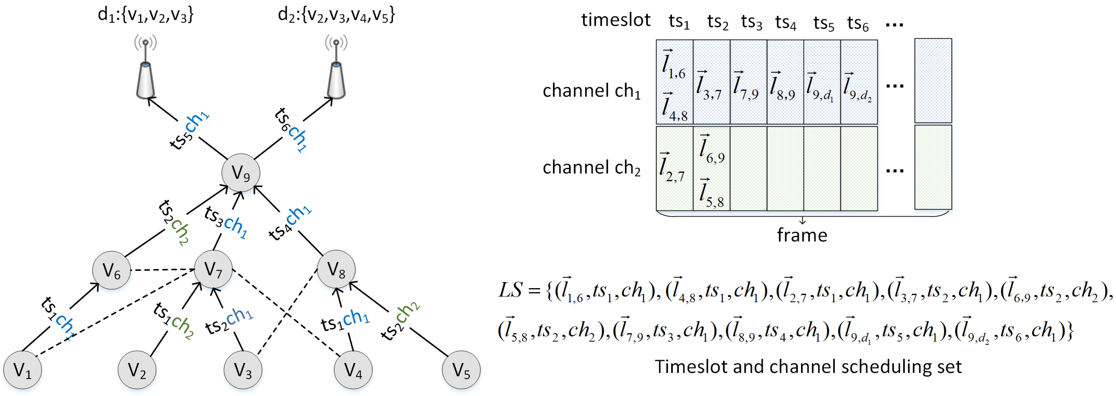
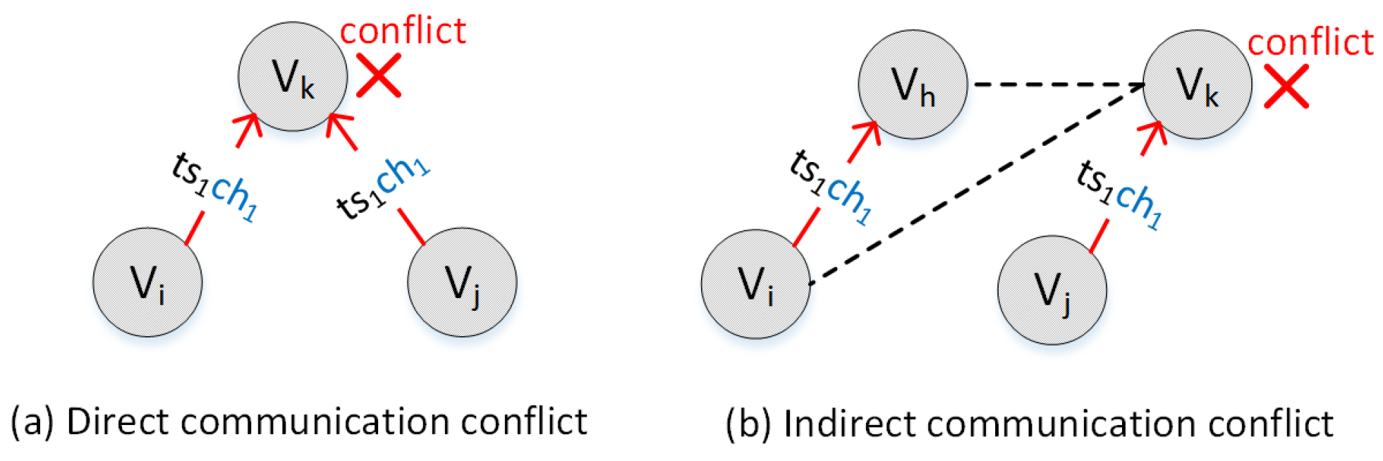
• Multi-channel WSN environment has been, firstly, introduced into the research of many-to-many data aggregation scheduling up to now. The characteristics of this new type of scenario are sufficiently considered in this paper, such as that an intermediate node is probably assigned to multiple transmission times, and some communication conflicts can be avoided by switching channel.
• The scheduling process of many-to-many data aggregation in a multi-channel WSN is formulated to decentralized, partially observable Markov decision process, as a result of summarizing its distinguishing features of wireless communication. A multi-agent is viewed as the nodes participating in wireless communication, and the system state cannot be accurately obtained by agents.
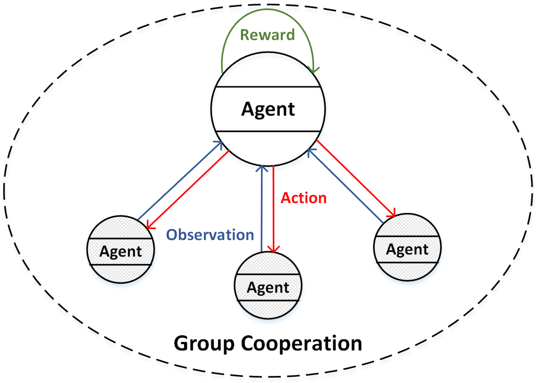
• Cooperative multi-agent learning is introduced to implement a new distributed scheduling method. Thanks to the property of group observability, a group of sensor nodes within one hop can attempt different behaviours and receive corresponding feedback. After accumulating adequate experience, sensor nodes learn the best action strategy and select the most efficient time slot and channel for wireless communication.

For understanding the proposed new method further, it is necessary to clarify the mutual relationships among these mentioned technical terms. The function of data aggregation scheduling is to allocate the time slot and channel resources to sensor nodes, where data aggregation as the data-processing operation is applied on the sensor nodes to reduce data traffic during data transmission. Multi-agent learning is an intelligent algorithm running on sensors to help sensors learn the best scheduling policy and exploit the most efficient time slot and channel.

The rest of the paper is organized as follows: Section 2 compares and analyses the shortcomings of the existing research. Section 3 introduces the concerned system model and illustrates the problems which are aimed to be solved in this paper. Section 4 explains the principle and components of the proposed many-to-many data aggregation scheduling method for a multi-channel WSN. Section 5 displays the simulation platform and analyses the simulation result in order to prove the high performance of the proposed policy. Finally, Section 6 concludes the current work. The abbreviations of the utilized technical terms are listed in the Appendix A.

2. Related Works

Existing data aggregation scheduling methods mainly focus on traditional WSN with exclusive wireless channel and many-to-one communication modes [12,17]. Generally speaking, there are two types of existing scheduling methods in WSN. The centralized-computing-based methods are normally operated on a sink node or a base station, which collects the global network information and computes the scheduling result with good performance [18]. The distributed-based methods are lightweight and deployed on sensor nodes [19]; the scheduling result is computed by the cooperation of many nodes with local information.

S. Kumar et al. propose the multi-channel TDMA scheduling algorithm with the objective of minimizing the total energy consumption in the network [20]. In order to alleviate collisions and support concurrent communications, multiple RF channels are utilized. The proposed heuristic algorithms offer computationally efficient scheduling operation, although they provide sub-optimum schedules for data gathering. J. Ma et al. study the continuous link scheduling problem in WSN [21], in which each node is assigned continuous time slots, so that the node can only wake up once in a scheduling cycle to complete its data-collection task. Many-to-many communication scheduling problems for battery-free WSN were firstly concerned by B. Yao et al., where energy bottlenecks were analysed, and an energy-adaptive and bottleneck-aware scheduling algorithm was proposed as well [22]. Bagaa et al. proposed a cross-layer trusted data aggregation scheduling method for a multi-channel WSN [23]. This method constructs k disjoint paths for each source node to the sink node based on the aggregation tree at first, and then finds a conflict-free communication schedule according to a routing structure. Jiao et al. firstly proved that the data aggregation scheduling problem for multi-channel duty cycle wireless sensor networks is NP-hard [24]; this research adopts the candidate-activity conflict and feasible-activity conflict graph to describe the node scheduling relationship, and, finally, used the coloring method to achieve efficient scheduling. Nevertheless, there are several common premises to achieve data aggregation scheduling using these centralized computing methods. First of all, a certain powerful base station has to take responsibility to collect global network information and compute a good scheduling plan. Once a network structure has undergone any change, global network information must be collected again, and a scheduling algorithm has to be re-executed. Moreover, the time of all the network nodes must be synchronized with high precision in advance. It is difficult to meet such requirements in large-scale wireless sensor networks.

A few researchers have designed distributed data aggregation scheduling method for multi-channel WSNs. B. Kang et al. [19] developed a distributed delay effective scheduling method to solve the problem of time slot scheduling in duty cycle wireless sensor networks. This method makes full use of duty cycle technology to appropriately turn off node communication and sensing capabilities. The active time of nodes is significantly reduced, and the lifetime of the network is apparently extended. Y. Lu et al. integrates an independent Q learning technique into the exploring process of an adaptive time slot scheduling for many-to-one application; the scheduling gradually approaches the optimal result along with the execution of frames [25]. A cluster-based distributed data aggregation scheduling algorithm with multi-power and multi-channel is proposed by Ren M. et al. in [26], which puts network nodes into multiple clusters, and uses different power levels for inner cluster communications and the communications among cluster heads separately. Moreover, communication latency caused by conflicts is reduced a lot due to the allocations of multiple channels. In order to minimize the time slot length of multi-channel wireless multi-hop wireless sensor networks, Lee et al. propose a conflict-free TDMA link scheduling method [27], using min–max to optimize the time-slot length, and minimize the end-to-end delay using a sorting algorithm. Nevertheless, these scheduling methods are designed for the communication pattern with a single sink, and they cannot be directly applied for many-to-many communication. Yu B. et al. consider the minimum-time aggregation scheduling problem in multi-sink sensor networks to support many-to-many data aggregation for the first time [28], where the bounds of the aggregation time are analyzed by a theoretical model, and they propose a nearly constant approximation algorithm to solve the aforementioned problem. Saginbekov S. et al. [10] designs a time-slot scheduling method with data aggregation for two sink nodes, but they do not discuss the feasibility and performance of their method for the scenarios with more sinks. Meanwhile, the multi-channel environment is not taken into account in this research.

In conclusion, there has been no existing work that directly researches many-to-many data aggregation scheduling methods for multi-channel WSN until now; in particular, the scheduling method needs to be implemented in a distributed manner to support a dynamic and extensible network environment.

3. System Model and Problem Statement

3.1. System Model

A WSN can be abstracted as a graph $G\left(V,\overrightarrow{L}\right)$ where V and $\overrightarrow{L}$ denote the set of sensor nodes and the set of communication links (edges), respectively. Sensor nodes use a half-duplex transmission mode, where one node cannot perform data transmission and data reception at the same time. If any pair of nodes $v_i\in V$ and $v_j\in V$ are located within the wireless communication range of each other, both links ${\overrightarrow{l}}_{i,j}\in \overrightarrow{L}$ and ${\overrightarrow{l}}_{j,i}\in \overrightarrow{L}$ exist in network. The nodes located in the wireless communication range of $v_i$ are called called neighbors $ngh\left(v_i\right)$. There are $\left|CH\right|$ available wireless channels, and $c{h}_k$ denotes the $k_{th}$ channel. For simplicity, the protocol interference model is adopted in this system, the communication radius $r_{cm}$ and the interference radius $r_{it}$ of each sensor node are set to the same value. Some sensors cannot transmit data simultaneously within the same wireless channel on account of communication conflicts. The utilized notations and variables are listed in Appendix B.

Sensing data produced on each source node is delivered to a set of sink or destination nodes; meanwhile, a sink node $d_i$ expects to collect the data from a set of source nodes. For example, sink node $d_1$ expects to collect sensing data from a set of source nodes $d_1=\{v_1,v_2,v_3\}$ in Figure 1. Intermediate nodes between source and sink nodes are going to perform data aggregation and forward the processed result. The communication period is defined as a frame $T{S}_c$, which consists of a fixed number of time slots $ts$. The fundamental task of the scheduling method is to allocate a time slot and wireless channel for each node without a communication conflict in order to maximize network performance. In this scenario, two kinds of potential conflict may appear in a network. The first one is direct conflict, where two or more links which possess at least one exact same terminal are allocated for the same time slot, and this overlapping terminal cannot concurrently handle two or more communication tasks at the same time slot, so the communication conflict appears. An example is depicted in Figure 2a, ${\overrightarrow{l}}_{i,k}$ and ${\overrightarrow{l}}_{j,k}$ have the same receiving terminal $v_k$, the same allocated time slot $t{s}_1$ will lead to the generation of communication conflict on $v_k$. Second one is indirect conflict: the receiving terminal of one link is located in the interfering range of the transmitting terminal of another link, and both links are allocated the same time slot and channel; then, the indirect communication conflict appears. An example is depicted in Figure 2b, $v_k$ is located in the interference range of $v_i$; once the same timeslot $t{s}_1$ and channel $c{h}_1$ are allocated to both ${\overrightarrow{l}}_{i,h}$ and ${\overrightarrow{l}}_{j,k}$, an indirect communication conflict happens on $v_k$.

In each time slot, the links without any conflict could perform wireless communication together. The links with the same time slot but also with the indirect conflicts could be allocated for different wireless channels. Once a data packet is successfully transmitted to a receiver, the  corresponding transmitter is supposed to obtain an acknowledgement (ACK) packet from this receiver inside the same time slot and channel. An example is shown in Figure 1: Solid lines represent the links with data transmission. Dashed lines indicate the links without data transmission, which is not the path of data routing. Links ${\overrightarrow{l}}_{1,6}$ and ${\overrightarrow{l}}_{4,8}$ without any conflict are allowed to be concurrently performed in the time slot $t{s}_1$ and the channel $c{h}_1$. ${\overrightarrow{l}}_{2,7}$ has to use the channel $c{h}_2$ because it has indirect conflict with ${\overrightarrow{l}}_{1,6}$, where $v_7$ is located in the interfering range of $v_1$.

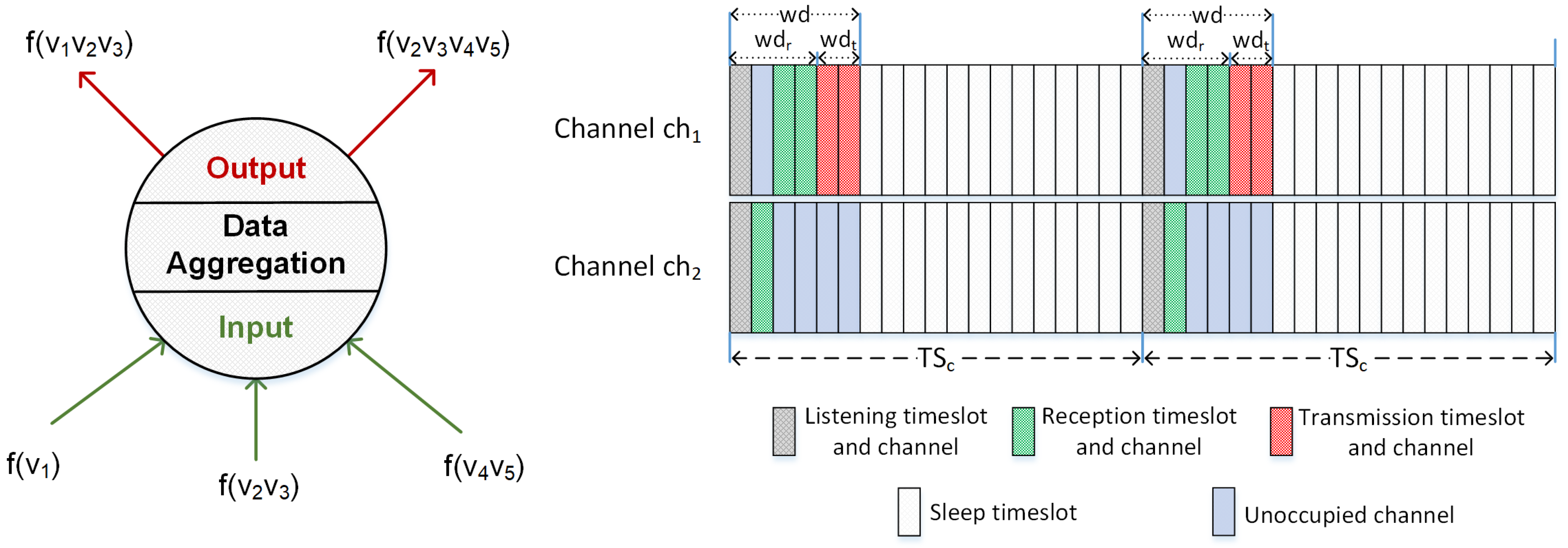
3.2. Optimization Objective

Even though a WSN routing protocol is not the main research contents of this paper, our system model requires that each node possesses local routing information before many-to-many data aggregation scheduling. In order to maintain consistency with the scheduling optimization objective, MUSTER as a classical distributed routing protocol for many-to-many data aggregation is adopted in our model [29], so that a routing structure with less transmission delay and less energy consumption can be constructed before allocating a time slot and channel.

In this case, a node $v_i$ has the knowledge of its upstream $US\left(v_i\right)$ and downstream nodes $DS\left(v_i\right)$ in the routing structure. Thanks to the property of the data aggregation function, the data from multiple receiving packets towards the same sink could be combined into a single data copy, such as $v_8$ in Figure 1 which is able to combine the packets from $v_4$ and $v_5$. In addition, the existence of multiple sinks probably makes one node take multiple transmission operations, such as $v_9$ having to transmit two packets to different next-hop nodes. Figure 3 focuses on this data aggregation operation, where $f\left(v_2{v}_3\right)$ represents the aggregation results of source nodes $v_2$ and $v_3$. This node receives three input packets, then performs a data aggregation function, and, finally, generates two aggregation results as output packets $f\left(v_1{v}_2{v}_3\right)$ and $f\left(v_2{v}_3{v}_4{v}_5\right)$ towards $d_1$ and $d_2$, respectively.

From the viewpoint of a global network, many-to-many data aggregation scheduling for an entire network in a frame is set to allocate a time slot and channel for each link with a data transmission task, and then the link-based scheduling set can be expressed as $LS=\{{\overrightarrow{ls}}_{i,j},\cdots \}$, which consists of the resource allocation sets ${\overrightarrow{ls}}_{i,j}$ for each link, where $\left|LS\right|$ is equal to the number of links $\left|L\right|$. ${\overrightarrow{ls}}_{i,j}=({\overrightarrow{l}}_{i,j},t{s}^{i,j},c{h}^{i,j})$ denotes the resource allocation set for the link ${\overrightarrow{l}}_{i,j}$ including the allocated time slot $t{s}^{i,j}$ and the allocated channel $c{h}^{i,j}$; an example can be found in Figure 1, where $l{s}_{1,6}=({\overrightarrow{l}}_{1,6},t{s}_1,c{h}_1)$, $t{s}^{1,6}=t{s}_1$ and $c{h}^{1,6}=c{h}_1$.

There is a specified time period in one frame which is called working window $wd$. During $wd$, a sensor node maintains an active state to conduct wireless communication, computation and other operations. $wd$ is further divided into reception slice $w{d}_r$ and transmission slice $w{d}_t$. According to the feature of data aggregation, the current node switch on the radio receiver during $w{d}_r$, the data packets from upstream nodes are supposed to be received from any wireless channel, and the aggregated result is obtained at the end of $w{d}_r$. After that, the current node starts to deliver the results to downstream nodes during $w{d}_t$. For a node $v_i$, the length of $wd$ is equal to $|w{d}_r|+|w{d}_t|$, which is directly related to the number of upstream and downstream nodes. $|w{d}_r|$ is set as $|US\left(v_i\right)|+⌊\left|US\right(v_i\left)\right|/2⌋$, where $⌊\left|US\right(v_i\left)\right|/2⌋$ is an additional amount to enhance the success rate of packet reception. $|w{d}_t|$ is strictly equal to the number of downstream nodes $DS\left(v_i\right)$, and each time slot is allowed to conduct one time of transmission. Besides working windows, the current node remains in an inactive or sleep state and temporarily switches off power supply for primary electronic units, this behavior helps to effectively save energy.

The allocation of many-to-many data aggregation for one node can be expressed as a scheduling tuple with two parameters $(w{d}_t.end,C{H}_u)$, where $w{d}_t.end$ denotes the end of transmission slice and $C{H}_u$ denotes the channel usage set. Since the size of $wd$ is fixed, $w{d}_t.end$ as the last timeslot directly decides the location of $wd$ in a frame, it is also indicates which timeslots are used for reception or transmission. $C{H}_u$ is a channel sequence $\{c{h}^{i,j},\cdots \}$ to specify the channel for each transmission timeslot. Figure 3 depicts an example of the scheduling operation on $v_9$ of Figure 2, where the scheduling tuple is $(t{s}_5,\{c{h}_1,c{h}_1\})$.

Multiple optimization objectives of scheduling are considered in this paper, and these objectives can be alternated according to the real-life application demand. For example, if communication delay is decreased, residual energy of nodes should be increased. Let ${\eta }_k$ represent $k^{th}$ or the last objective function; then, the scheduling problem is expressed as $\underset{LS}{argmin}\left\{\phi ({\eta }_1\left(LS\right),\cdots ,{\eta }_k\left(LS\right))\right\}$, where $\phi$ denotes the overall objective function, $RS$ denotes the routing structure (set), and the solution should be subject to the following constraints:

• $(LS-l{s}_{i,j})\cap l{s}_{i,j}=⌀,\forall {\overrightarrow{l}}_{i,j}\in RS$
• If ${\overrightarrow{l}}_{i,j}\in RS$, $\forall {\overrightarrow{l}}_{i,m}\in RS$ or ${\overrightarrow{l}}_{n,j}\in RS$, then $l{s}_{i,m}.t{s}^{i,m}\ne l{s}_{i,j}.t{s}^{i,j}$ or $l{s}_{n,j}.t{s}^{n,j}\ne l{s}_{i,j}.t{s}^{i,j}$
• If ${\overrightarrow{l}}_{i,j}\in RS$, $\forall {\overrightarrow{l}}_{i,m}\in \overrightarrow{L}$ and $\notin RS,{\overrightarrow{l}}_{n,m}\in \overrightarrow{L}$, then $l{s}_{i,j}.t{s}^{i,j}\ne l{s}_{n,m}.t{s}^{n,m}$ or $l{s}_{i,j}.c{h}^{i,j}\ne l{s}_{n,m}.c{h}^{n,m}$
• $w{d}_r.end\left(v_i\right)<w{d}_t.first\left(v_i\right),\forall v_i\in V$
• $w{d}_t.end\left(US\left(v_i\right)\right)<w{d}_t.end\left(v_i\right)<w{d}_t.end\left(DS\left(v_i\right)\right),\forall v_i\in V$

The first constraint requires that communication on each link can only be performed once, so the allocation of the slot and channel for one link $l{s}_{i,j}$ is unique. The second constraint indicates the avoidance of direct interference; when a certain link ${\overrightarrow{l}}_{i,j}$ activates communication, then any link with the same terminals cannot perform communication in the same time slot. The third constraint indicates the avoidance of indirect interference: the links with interference cannot share the same time slot or the same channel. The fourth constraint is generated from the principle of data aggregation, where an aggregated result is supposed to be transmitted after receiving all expected data. The last constraint explains that the transmission operation of the current node should be located between its downstream node and its upstream node. It is evident that the essence of the scheduling problem is to find the best set of links that satisfies the optimization goals and constraints. This is a typical combinatorial optimization problem that can be solved by reinforcement learning methods [30]. Besides these constraints, transmission delay and energy consumption as the optimization objectives of many-to-many data aggregation scheduling are selected in this paper.

3.3. Decentralized Partially Observable Markov Decision Process

By summarizing the characteristics of many-to-many data aggregation scheduling for a multi-channel WSN, it is not difficult to find a match between this scheduling process and the decentralized partially observable Markov decision process (Dec-POMDP) [31]. Dec-POMDP can be formulated as $〈I,S,A,P,R,\Omega ,O,b,T〉$, which is a tuple and its components are described as follows:

• $I=\{1,2,...,\left|V\right|\}$ is the set of agents; one sensor node participating in communication is viewed as one agent.
• $S=S_1\times S_2\times ...S_{\left|V\right|}$ is a finite set of system or joint states where $\overrightarrow{s}=\{s_1,s_2,..s_{\left|V\right|}\},\overrightarrow{s}\in S,S_i$ is the state set of the $i^{th}$ agent, which reflects whether the reception and transmission of packets on this node is successful, and this information cannot be accurately acquired due to the environment of wireless communication.
• $A=A_1\times A_2\times ...A_{\left|V\right|}$ is a finite set of joint actions where $\overrightarrow{a}=\left\{a_1,a_2,..a_{\left|V\right|}\right\},a\in A,A_i$ is the action set of the $i^{th}$ agent. The change in scheduling for time slot and channel is realized by modifying the tuple mentioned before $(w{d}_t.end,C{H}_u)$.
• $P\left({\overrightarrow{s}}^{\prime }\right|\overrightarrow{s},\overrightarrow{a})$ is the transition function which denotes the probability of transitioning from the state $\overrightarrow{s}$ to the new state ${\overrightarrow{s}}^{\prime }$ when taking the joint action $\overrightarrow{a}$.
• $R(\overrightarrow{s},\overrightarrow{a})$ is the reward function which denotes the immediate reward when taking the joint action $\overrightarrow{a}$ at the state $\overrightarrow{s}$.
• $\Omega ={\Omega }_1\times {\Omega }_2\times ..{\Omega }_{\left|V\right|}$ is a finite set of joint observations, ${\Omega }_i$ is the individual observation set of the $i^{th}$ agent, where a joint observation is $\overrightarrow{\omega }=\{{\omega }_1,{\omega }_2,...,{\omega }_{\left|V\right|}\},\overrightarrow{\omega }\in \Omega$. One observation ${\omega }_i$ contains the size and number information of the successfully received and transmitted packets, and this information is part of the acknowledgement packet.
• $O\left({\overrightarrow{\omega }}^{\prime }\right|{\overrightarrow{s}}^{\prime },\overrightarrow{a})$ is the observation function which denotes the probability of observing ${\overrightarrow{\omega }}^{\prime }$ when the system state transfers to $\overrightarrow{s}$ by taking the joint action $\overrightarrow{a}$. Due to the wireless communication environment, the observation result may not truly reflect the system state, because the reception of ACK cannot ensure no error is contained in transmission data; meanwhile, not receiving ACK also cannot determine whether the receiving node did not obtain data.
• $b=b_1\times b_2\times \cdots b_{\left|V\right|}$ is the initial system state distribution (also called the initial belief), for the system state $\overrightarrow{s},b\left(\overrightarrow{s}\right)={\prod }_{i\in I)}{b}_i\left(s_i\right)$, where $b_i$ is the initial state distribution over $S_i$.
• T is the finite horizon or the number of time steps in which an agent can interact with Dec-POMDP model.

In a specific system state ${\overrightarrow{s}}^t$ at time step t, a joint observation ${\overrightarrow{\omega }}^t$ can be generated. Each agent obtains its individual observation ${\omega }_i^t$, and selects its individual action $a_i^t$ which is a component of a joint action ${\overrightarrow{a}}^t$. After taking action, the system transitions to the next state ${\overrightarrow{s}}^{t+1}$, and each agent obtains its immediate reward r. The action-observation history of the $i^{th}$ agent is denoted as ${\Phi }_i^t=({\omega }_i^0,a_i^0,{\omega }_i^1,a_i^1,...,a_i^{t-1},{\omega }_i^t)$, so the joint action-observation history is denoted as ${\overrightarrow{\Phi }}^t=〈{\Phi }_1^t,{\Phi }_2^t,...,{\Phi }_{\left|V\right|}^t〉$. Agent policy uses history to decide actions, which is denoted as ${\pi }_i:{\Phi }_i\to A_i$, and a joint policy $\pi =〈{\pi }_1,{\pi }_2,...,{\pi }_{\left|V\right|}〉$ is the combination of all individual policies. The final goal of solving Dec-POMDP is to discover an optimal joint policy in order to maximize the expected accumulated discounted reward; the state value function $V^{\pi }\left(\overrightarrow{s}\right)$ of a joint policy $\pi$ from state $\overrightarrow{s}$ is defined as follows:

$$V^{\pi }\left(\overrightarrow{s}\right)=E\left[\sum _{t=0}^{h-1}{\gamma }^{t}R({\overrightarrow{s}}^t,{\overrightarrow{a}}^t)|\overrightarrow{s},\pi \right]$$

(1)

where $\gamma$ is the discounted factor to decide the importance or weight of the future rewards, and if $\gamma =0$, then only the current reward is considered in the value function. To obtain such a policy, the reinforcement-learning algorithm normally evaluates an action quality by Q-function or Q-value function $Q({\overrightarrow{s}}^t,{\overrightarrow{a}}^t)$, which is denoted as follows:

$$\begin{array}{cc}\hfill Q({\overrightarrow{s}}^t,{\overrightarrow{a}}^t)=& R({\overrightarrow{s}}^t,{\overrightarrow{a}}^t)+\hfill \\ \hfill & \underset{\pi }{max}\sum _{{\overrightarrow{s}}^{t+1}}P\left({\overrightarrow{s}}^{t+1}\right|{\overrightarrow{s}}^t,{\overrightarrow{a}}^t)V^{\pi }\left({\overrightarrow{s}}^{t+1}\right)\hfill \end{array}$$

(2)

However, it is impossible to let agents obtain accurate system state $\overrightarrow{s}$, so the basic edition of Q-learning cannot be directly applied for Dec-POMDP. In this case, the action-observation history is applied to replace the system state, and the updated rule of Q-value can be denoted as follows:

$$\begin{array}{cc}\hfill Q({\overrightarrow{\Phi }}^t,{\overrightarrow{a}}^t)=& (1-\alpha )Q({\overrightarrow{\Phi }}^t,{\overrightarrow{a}}^t)+\hfill \\ \hfill & \alpha [R({\overrightarrow{\Phi }}^t,{\overrightarrow{a}}^t)+\gamma \underset{\overrightarrow{a}\in A}{max}Q({\overrightarrow{\Phi }}^{t+1},\overrightarrow{a})]\hfill \end{array}$$

(3)

where $\alpha$ is the learning rate to control the updating speed of the Q-value. The optimal policy can be found to make the action decision on agents, which can be expressed as follows:

$${\pi }^{*}\left(\overrightarrow{\Phi }\right)=\underset{\overrightarrow{a}\in A}{argmax}Q(\overrightarrow{\Phi },\overrightarrow{a})$$

(4)

4. Many-to-Many Data Aggregation Scheduling Based on Multi-Agent Learning

4.1. Group Cooperation

Regardless of the discovery of the optimal scheduling set or the optimal action policy for slot and channel allocation, the global information of the entire WSN is a common prerequisite. However, to acquire global information is almost impossible in such a dynamic network environment; meanwhile, the spaces of action, observation, and policy are exponential in the number of agents. One feasible method is distributed independent learning, in which agents only utilize their own observations and rewards, and ignore other agents’ information. However, without considering the cooperation of agents, this type of method cannot ensure the quality of the solution; thus, probably performing the scheduling with inferior performance.

To address the mentioned issues further, the core idea of a multi-agent learning with group observability for Dec-POMDP in [32] can be exploited for designing an efficient many-to-many data aggregation scheduling method. By building a number of agent groups, it is possible to split the global function into the group functions. Due to the existence of a WSN routing structure, a group can be naturally constructed by the nodes within one hop. The downstream node for data transmission is automatically selected as group head, when there are multiple downstream nodes; only the node with the largest identity number is recognized as group head for a current node. Meanwhile, the upstream nodes are group members, which are supposed to transmit their own observations to the group head. An example can be found in Figure 4. This method distributes the learning tasks by utilizing the interactions inside the routing structure $RS$, and it makes the learning agents cooperate in order to ensure the global performance, and its feasibility is proved by Theorem 1 in Section 4.5. A decomposable Q-function $\overline{Q}({\overrightarrow{\Phi }}^t,{\overrightarrow{a}}^t)$ is designed to represent the global Q-function $Q({\overrightarrow{\Phi }}^t,{\overrightarrow{a}}^t)$, and the former can be defined as the sum of the group Q-function:

$$\overline{Q}({\overrightarrow{\Phi }}^t,{\overrightarrow{a}}^t)=\sum _{g\in RS}{Q}_g({\overrightarrow{\Phi }}_g^t,{\overrightarrow{a}}_g^t)$$

(5)

where $Q_g({\overrightarrow{\Phi }}_g^t,{\overrightarrow{a}}_g^t)$ is the expected rewards for a group of agents after performing a joint group action ${\overrightarrow{a}}_g^t$ with a group history ${\overrightarrow{\Phi }}_g^t$. The relationship between $\overline{Q}({\overrightarrow{\Phi }}^t,{\overrightarrow{a}}^t)$ and $Q({\overrightarrow{\Phi }}^t,{\overrightarrow{a}}^t)$ is proved by Lemma 2 in Section 4.5. The update rule of the Q-function in Equation (3) can be rewritten as follows:

$$\begin{array}{cc}\hfill \sum _{g\in RS}{Q}_g({\overrightarrow{\Phi }}_g^t,{\overrightarrow{a}}_g^t)& =(1-\alpha )\sum _{g\in RS}{Q}_g({\overrightarrow{\Phi }}_g^t,{\overrightarrow{a}}_g^t)+\hfill \\ \hfill & \alpha [\sum _{g\in RS}R({\overrightarrow{\Phi }}_g^t,{\overrightarrow{a}}_g^t)+\gamma \underset{\overrightarrow{a}\in A}{max}\overline{Q}({\overrightarrow{\Phi }}^{t+1},\overrightarrow{a})]\hfill \end{array}$$

(6)

As the discounted future reward, even though global information cannot be directly obtained to compute $\underset{\overrightarrow{a}\in A}{max}\overline{Q}({\overrightarrow{\Phi }}^{t+1},\overrightarrow{a})$, the latter can be expressed by decomposing the optimal joint action ${\overrightarrow{a}}^{*}=\underset{\overrightarrow{a}\in A}{argmax}\overline{Q}(\overrightarrow{\Phi },\overrightarrow{a})$, where ${\overrightarrow{a}}^{*}={\bigcup }_{g\in RS}{\overrightarrow{a}}_g^{*}$; finally, $\underset{\overrightarrow{a}\in A}{max}\overline{Q}({\overrightarrow{\Phi }}^{t+1},\overrightarrow{a})$ can be rewritten as follows:

$$\underset{\overrightarrow{a}\in A}{max}\overline{Q}({\overrightarrow{\Phi }}^{t+1},\overrightarrow{a})=\overline{Q}({\overrightarrow{\Phi }}^{t+1},{\overrightarrow{a}}^{*})=\sum _{g\in RS}{Q}_g({\overrightarrow{\Phi }}_g^{t+1},{\overrightarrow{a}}_g^{*})$$

(7)

Benefiting from the decomposition, the update rule of group Q-function can be formulated as follows:

$$\begin{array}{cc}\hfill Q_g({\overrightarrow{\Phi }}_g^t,{\overrightarrow{a}}_g^t)=& (1-\alpha )Q_g({\overrightarrow{\Phi }}_g^t,{\overrightarrow{a}}_g^t)+\hfill \\ \hfill & \alpha [R({\overrightarrow{\Phi }}_g^t,{\overrightarrow{a}}_g^t)+\gamma Q_g({\overrightarrow{\Phi }}_g^{t+1},{\overrightarrow{a}}_g^{*})]\hfill \end{array}$$

(8)

During the learning process of an agent group g at time step t, after taking the joint action ${\overrightarrow{a}}_g^t$, group members transmit their own observations to the group head, and then the group head receives its group reward signal $R({\overrightarrow{\Phi }}_g^t,{\overrightarrow{a}}_g^t)$. After updating the action-observation history ${\overrightarrow{\Phi }}_g^{t+1}$, the group head computes the next optimal action ${\overrightarrow{a}}_g^{*}$ for ${\overrightarrow{\Phi }}_g^{t+1}$ using the distributed constraint optimization (DCOP) technology in [33], and then it distributes the next action to group members, which may execute ${\overrightarrow{a}}_g^{*}$ or explore actions. In this way, the global Q-function is decomposed into multiple local Q-functions on group heads. The selection of a group action is computed in a distributed manner with local group information.

4.2. Reward Function

The scheduling optimization for the objectives and constraints in Section 3.2 can be embodied in the reward function. The total reward of a group can be considered as the product of the rewards from group history and action, where $R({\overrightarrow{\Phi }}_g^t,{\overrightarrow{a}}_g^t)=R_{hs}\left({\overrightarrow{\Phi }}_g^t\right)R_{at}\left({\overrightarrow{a}}_g^t\right)$. The reward from group history $R_{hs}\left({\overrightarrow{\Phi }}_g^t\right)$ is affected by the numbers $n_r$, $n_t$ and the size $m^t$ of the successfully received and transmitted packets; this information is attached to the ACK packet. In general, the more numbers with a larger size of successfully received and transmitted packets are definitely helpful for reducing the energy consumption of nodes; as the probability of packet re-transmission will be significantly decreased, fewer conflicts will appear. $sg{n}_1(n_r,n_t)$ as an signum function is adopted to control the value of $R_{hs}\left({\overrightarrow{\Phi }}_g^t\right)$. If $n_r=US\left(v_i\right)$ and $n_t=DS\left(v_i\right)$, then $sg{n}_1\left(n\right)=1$; this means that the current node receives all the expected packets from upstream nodes and all outgoing packets are successfully transmitted to downstream nodes. Otherwise, not all the expected packets are successfully received or transmitted; then, $sg{n}_1(n_r,n_t)=0$. Let us assume the maximum packet capacity is $m_{max}^t$, then $R_{hs}\left({\overrightarrow{\Phi }}_g^t\right)$ can be defined as in the following equation.

$$R_{hs}\left({\overrightarrow{\Phi }}_g^t\right)=sg{n}_1(n_r,n_t)\prod _{i=1}^{n_r+n_t}(1+(\left(m_i^t\right)/\left(m_{max}^t\right)))$$

(9)

The reward from group action $R_{at}\left({\overrightarrow{a}}_g^t\right)$ has impacting factors containing the number of overlapped transmission time slots, and the position of the last transmission time slot. The first factor is a strict constraint to avoid communication conflicts in a group, and it directly decides whether a reward value is positive or not. The second factor is a typical index for communication delay; if this value is smaller, then a group has a higher chance of achieving a smaller communication delay. Finally, according to the previous definition of transmission window $w{d}_t$, the reward from a group action can be defined as follows:

$$R_{at}\left({\overrightarrow{a}}_g^t\right)=sg{n}_2(\left|\bigcap _{v_i\in g}w{d}_t\left(v_i\right)\right|)\sum _{v_i\in g}{e}^{(1/((w{d}_t.end\left(v_i\right))}$$

(10)

where ${\bigcap }_{v_i\in g}w{d}_t\left(v_i\right)$ denotes the intersection of the time slot set of a transmission window on each group member, and $sg{n}_2$ is another signum function. If ${\bigcap }_{v_i\in g}w{d}_t\left(v_i\right)$ is empty, it means that the transmitting nodes has no overlapping time slot; then, the reward value is positive where $sn{g}_2=1$. Otherwise, a communication conflict appears, the reward becomes a punishment and its value should be negative where $sn{g}_2=-1$. $w{d}_t.end\left(v_i\right)$ indicates the final transmission delay on the current node, and its value is expected to decrease.

4.3. Action Policy

The capability of random exploration of reinforcement learning should be maintained; then, the scheduling method has some probability to choose a random action instead of the optimal action. To match the convergent characteristic of learning, even though the random exploring range is normally required to be large at the earlier stages of learning, the random action probability should be decreased along with an increase in time steps. By making the parameter of the classic $ϵ-greedy$ policy alterable, the mentioned goal can be achieved. The adopted alterable parameter of selection probability ${\widehat{ϵ}}_t$ is correlated to the time steps t, which can be denoted as follows:

$${\widehat{ϵ}}_t=\frac{1}{\sigma (1+e^t)}$$

(11)

where $\sigma$ is a shrinking factor, and, along with the increase in time steps, the probability of random action become very little.

4.4. Many-to-Many Data Aggregation Scheduling Procedure

Algorithm 1 illustrates the execution process of the many-to-many data aggregation method. Horizon T, which controls the end of time steps, is a limited number. At the beginning of one frame, the current node executes $a_i^t$ or a random action to set the many-to-many data aggregation scheduling set on line 2. During the working window, if the current time slot is a reception time slot, then a packet is going to be received. On line 5-6, a group action ${\overrightarrow{a}}_g^{*}$ to group members is received; then, the individual action $a_i^t$ can be extracted from ${\overrightarrow{a}}_g^{*}$. On line 9-18, if an individual observation ${\omega }_i^t$ to a group head is received, then the information is stored. Once a group head has received all observations from its members, group observations ${\overrightarrow{\omega }}_g^t$ are subsequently constructed from memory; then, the group reward $R({\overrightarrow{\Phi }}_g^t,{\overrightarrow{a}}_g^t)$ can be obtained from the local environment, and the group history ${\overrightarrow{\Phi }}_g^{t+1}$ can be updated. The next optimal group action ${\overrightarrow{a}}_g^{*}$ can be computed by using DCOP, and the group Q-value is also updated. After that, ${\overrightarrow{a}}_g^{*}$ is attached to ACK and transmitted to all group members. On line 19–25, if the current time slot is a transmission time slot, data packets are supposed to be transmitted to all downstream nodes. When $v_j$ is the last downstream node in $DS\left(v_i\right)$, individual observation ${\omega }_i^t$ is obtained and attached to the data packet. Finally, the data packet is delivered to $v_j$.

Algorithm 1 Many-to-many data aggregation scheduling procedure.

1: for step $t=1$ to T on agent $v_i$ do 2:    executes $a_i^t$ or random action based on Equation (11); 3:    for timeslot $ts=1$ to $T{S}_c$ do 4:      if $ts\in w{d}_r$ then 5:         if $v_i$ receives ${\overrightarrow{a}}_g^{*}$ then 6:           decompose ${\overrightarrow{a}}_g^{*}$ to individual action $a_i^t$; $v_i$ receives ${\omega }_j^t$ 7:         else if $v_i$ receives ${\omega }_t^i$ then 8:           store ${\omega }_j^t$ into memory; 9:           if all observations are received from group members then 10:              construct group observations ${\omega }_g^t$; 11:              obtain group reward $R({\overrightarrow{\Phi }}_g^t,{\overrightarrow{a}}_g^t)$ based on Equation (9) and (10); 12:              update group history ${\overrightarrow{\Phi }}_g^{t+1}$; 13:              compute optimal action ${\overrightarrow{a}}_g^{*}$ based on DCOP; 14:              update group Q-value $Q_g({\overrightarrow{\Phi }}_g^t,{\overrightarrow{a}}_g^t)$ based on Equation (8); 15:              attach ${\overrightarrow{a}}_g^t$ on ACK and transmit ACK to group members; 16:           end if 17:         end if 18:      end if 19:      if $ts\in w{d}_t$ then 20:         for $v_j\in DS\left(v_i\right)$ do 21:           $DS\left(v_i\right)\leftarrow DS\left(v_i\right)-v_j$; 22:           if $DS\left(v_i\right)==Ø$ then 23:              obtain individual observation ${\omega }_i^t$ and attach on data packet; 24:           end if 25:           transmit data packet to $v_j$; 26:         end for 27:      end if 28:    end for 29: end for

4.5. Theoretical Analysis

The time and space complexity of reinforcement-learning-based algorithms has already been discussed in [34]. The difference in our method is the group cooperation among agents, such as the selection of optimal group actions based on DCOP. In this case, the number of group members is an indispensable impact factor for the complexity. The upper bound of time complexity on each agent can be expressed as $O\left(t\left|g\right|\right)$, where t denotes the total number of time steps, and $\left|g\right|$ denotes the number of group members, as mentioned before. Correspondingly, the upper bound of the space complexity on each agent is expressed as $O\left(h\left|\omega \right|\left|a\right|\left|g\right|\right)$, where h denotes the number of recent observation histories for selecting an action, $\left|\omega \right|$ and $\left|a\right|$ represent the size of observation and action, respectively, and both values are fixed. According to the formulation of Dec-POMDP in Section 3.3, $\left|\omega \right|$ depends on the number of transmitted packets, and $\left|a\right|$ is decided by the fixed number of the involved parameters. Thanks to the distributed nature, the overhead of computation and memory are scattered; either the time complexity or the space complexity declines.

The theoretical feasibility of the proposed scheduling method is established only in the case that the global Q-function $Q({\overrightarrow{\Phi }}^t,{\overrightarrow{a}}^t)$ for a network system is the same as the decomposable Q-function $\overline{Q}({\overrightarrow{\Phi }}^t,{\overrightarrow{a}}^t)$, and this condition has to be verified by theoretical analysis. A global Q-function with system state variables $Q({\overrightarrow{s}}^t,{\overrightarrow{\Phi }}^t,{\overrightarrow{a}}^t)$ is considered, then it is proved to be decomposable; after that, the result helps to prove the above condition. For the convenience of expression, the probability of state and observation transition are abbreviated as follows:

$$P_i^t=P_i\left({\overrightarrow{s}}_i^{t+1}\right|{\overrightarrow{s}}_i^t,{\overrightarrow{a}}_i^t)O_i\left({\overrightarrow{\omega }}_i^{t+1}\right|{\overrightarrow{s}}_i^{t+1},{\overrightarrow{a}}_i^t)$$

(12)

According to the definition of the Bellman equation, $Q({\overrightarrow{s}}^t,{\overrightarrow{\Phi }}^t,{\overrightarrow{a}}^t)$ can be expressed as follows:

$$\begin{array}{cc}\hfill & Q({\overrightarrow{s}}^t,{\overrightarrow{\Phi }}^t,{\overrightarrow{a}}^t)=R({\overrightarrow{s}}^t,{\overrightarrow{a}}^t)+\hfill \\ \hfill & \gamma \sum _{{\overrightarrow{s}}^{t+1},{\overrightarrow{\Phi }}^{t+1}}{P}_1^t{P}_2^t\cdots P_{\left|V\right|}^t\underset{\overrightarrow{a}\in A}{max}Q({\overrightarrow{s}}^{t+1},{\overrightarrow{\Phi }}^{t+1},\overrightarrow{a})\hfill \end{array}$$

(13)

where ${\overrightarrow{\Phi }}^{t+1}$ is the ${\overrightarrow{\Phi }}^t$ appended by action ${\overrightarrow{a}}^t$ and observation ${\overrightarrow{\omega }}^t$, $\underset{\overrightarrow{a}\in A}{max}Q({\overrightarrow{s}}^{t+1},{\overrightarrow{\Phi }}^{t+1},\overrightarrow{a}))$ actually denotes $Q({\overrightarrow{s}}^{t+1},{\overrightarrow{\Phi }}^{t+1},{\overrightarrow{a}}^{*})$, and ${\overrightarrow{a}}^{*}$ is the global optimal joint action. For the time step t, $b^t$ is the belief or distribution, which completely depends on the initial belief b and history ${\overrightarrow{\Phi }}^t$; then, $Q({\overrightarrow{s}}^t,{\overrightarrow{\Phi }}^t,{\overrightarrow{a}}^t)$ transforms into the global Q-function without system state $Q({\overrightarrow{\Phi }}^t,{\overrightarrow{a}}^t)$:

$$Q({\overrightarrow{\Phi }}^t,{\overrightarrow{a}}^t)=\sum _{{\overrightarrow{s}}^t\in S}{b}^t\left({\overrightarrow{s}}^t\right)Q({\overrightarrow{s}}^t,{\overrightarrow{\Phi }}^t,{\overrightarrow{a}}^t)$$

(14)

By utilizing the above principle, the group Q-function with group state is defined as follows:

$$\begin{array}{cc}\hfill & Q_g({\overrightarrow{s}}_g^t,{\overrightarrow{\Phi }}_g^t,{\overrightarrow{a}}_g^t)=R({\overrightarrow{s}}_g^t,{\overrightarrow{a}}_g^t)+\hfill \\ \hfill & \gamma \sum _{{\overrightarrow{s}}_g^{t+1},{\overrightarrow{\Phi }}_g^{t+1}}{P}_{g_1}^t{P}_{g_2}^t\cdots P_{\left|g\right|}^t\underset{{\overrightarrow{a}}_g\in A_g}{max}Q({\overrightarrow{s}}_g^{t+1},{\overrightarrow{\Phi }}_g^{t+1},{\overrightarrow{a}}_g)\hfill \end{array}$$

(15)

In this way, the group Q-function without group state is, subsequently, defined as follows:

$$Q_g({\overrightarrow{\Phi }}_g^t,{\overrightarrow{a}}_g^t)=\sum _{{\overrightarrow{s}}_g^t\in S_g}{b}_g^t\left({\overrightarrow{s}}_g^t\right)Q_g({\overrightarrow{s}}_g^t,{\overrightarrow{\Phi }}_g^t,{\overrightarrow{a}}_g^t)$$

(16)

Lemma 1.

For any finite time step t in the Dec-POMDP model, the global Q-function with system state $Q({\overrightarrow{s}}^t,{\overrightarrow{\Phi }}^t,{\overrightarrow{a}}^t)$ is decomposable and equal to ${\sum }_{g\in RS}{Q}_g({\overrightarrow{s}}_g^t,{\overrightarrow{\Phi }}_g^t,{\overrightarrow{a}}_g^t)$.

Proof. 

Mathematical induction is adopted to prove this lemma. Firstly, let us assume that the following decomposition equation holds for the time step $t+1$,

$$Q({\overrightarrow{s}}^{t+1},{\overrightarrow{\Phi }}^{t+1},{\overrightarrow{a}}^{t+1})=\sum _{g\in RS}{Q}_g({\overrightarrow{s}}_g^{t+1},{\overrightarrow{\Phi }}_g^{t+1},{\overrightarrow{a}}_g^{t+1})$$

(17)

After that, let us analyse whether the decomposition equation for the time step t still holds; the derivation process is as follows:

$$\begin{array}{cc}\hfill & Q({\overrightarrow{s}}^t,{\overrightarrow{\Phi }}^t,{\overrightarrow{a}}^t)\hfill \\ \hfill & =R({\overrightarrow{s}}^t,{\overrightarrow{a}}^t)+\hfill \\ \hfill & \gamma \sum _{{\overrightarrow{s}}^{t+1},{\overrightarrow{\Phi }}^{t+1}}{P}_1^t{P}_2^t\cdots P_{\left|V\right|}^t\underset{\overrightarrow{a}}{max}Q({\overrightarrow{s}}^{t+1},{\overrightarrow{\Phi }}^{t+1},\overrightarrow{a})\hfill \\ \hfill & =\sum _{g\in RS}R({\overrightarrow{s}}_g^t,{\overrightarrow{a}}_g^t)+\hfill \\ \hfill & \gamma \sum _{{\overrightarrow{s}}^{t+1},{\overrightarrow{\Phi }}^{t+1}}{P}_1^t{P}_2^t\cdots P_{\left|V\right|}^{t}Q({\overrightarrow{s}}^{t+1},{\overrightarrow{\Phi }}^{t+1},{\overrightarrow{a}}^{*})\hfill \\ \hfill & =\sum _{g\in RS}R({\overrightarrow{s}}_g^t,{\overrightarrow{a}}_g^t)+\hfill \\ \hfill & \gamma \sum _{{\overrightarrow{s}}^{t+1},{\overrightarrow{\Phi }}^{t+1}}{P}_1^t{P}_2^t\cdots P_{\left|V\right|}^t\sum _{g\in RS}{Q}_g({\overrightarrow{s}}_g^{t+1},{\overrightarrow{\Phi }}_g^{t+1},{\overrightarrow{a}}_g^{*})\hfill \\ \hfill & =\sum _{g\in RS}\{R({\overrightarrow{s}}_g^t,{\overrightarrow{a}}_g^t)+\hfill \\ \hfill & \gamma \sum _{{\overrightarrow{s}}^{t+1},{\overrightarrow{\Phi }}^{t+1}}{P}_{g_1}^t{P}_{g_2}^t\cdots P_{\left|g\right|}^t{Q}_g({\overrightarrow{s}}_g^{t+1},{\overrightarrow{\Phi }}_g^{t+1},{\overrightarrow{a}}_g^{*})\}\hfill \\ \hfill & =\sum _{g\in RS}{Q}_g({\overrightarrow{s}}_g^t,{\overrightarrow{\Phi }}_g^t,{\overrightarrow{a}}_g^t)\hfill \end{array}$$

(18)

□

Lemma 2.

For any finite time step t in the Dec-POMDP model, the global Q-function without system state $Q({\overrightarrow{\Phi }}^t,{\overrightarrow{a}}^t)$ is decomposable and equal to ${\sum }_{g\in RS}{Q}_g({\overrightarrow{\Phi }}_g^t,{\overrightarrow{a}}_g^t)$.

Proof. 

According to Lemma 1 and Equation (15) and (18), the derivation process is as follows:

$$\begin{array}{cc}\hfill & Q({\overrightarrow{\Phi }}^t,{\overrightarrow{a}}^t)\hfill \\ \hfill & =\sum _{\overrightarrow{s}\in S}{b}^t\left(\overrightarrow{s}\right)Q({\overrightarrow{s}}^t,{\overrightarrow{\Phi }}^t,{\overrightarrow{a}}^t)\hfill \\ \hfill & =\sum _{\overrightarrow{s}\in S}{b}_1^t\left(s_1\right)b_2^t\left(s_2\right)\cdots b_{\left|V\right|}^t\left(s_{\left|V\right|}\right)Q({\overrightarrow{s}}^t,{\overrightarrow{\Phi }}^t,{\overrightarrow{a}}^t)\hfill \\ \hfill & =\sum _{\overrightarrow{s}\in S}{b}_1^t\left({\overrightarrow{s}}_1\right)b_2^t\left({\overrightarrow{s}}_2\right)\cdots b_{\left|V\right|}^t\left({\overrightarrow{s}}_{\left|V\right|}\right)\sum _{g\in RS}{Q}_g({\overrightarrow{s}}_g^t,{\overrightarrow{\Phi }}_g^t,{\overrightarrow{a}}_g^t)\hfill \\ \hfill & =\sum _{g\in RS}\sum _{{\overrightarrow{s}}_g^t\in S_g}{b}_g^t\left({\overrightarrow{s}}_g^t\right)Q_g({\overrightarrow{s}}_g^t,{\overrightarrow{\Phi }}_g^t,{\overrightarrow{a}}_g^t)\hfill \\ \hfill & =\sum _{g\in RS}{Q}_g({\overrightarrow{\Phi }}_g^t,{\overrightarrow{a}}_g^t)\hfill \end{array}$$

(19)

□

Theorem 1.

In Dec-POMDP model, the optimal policy ${\pi }^{*}\left(\overrightarrow{\Phi }\right)$ will be found by the proposed cooperative multi-agent learning method.

Proof. 

Based on the basic property of Q-learning and Equation (8), the group Q-function without group state $Q_g({\overrightarrow{\Phi }}_g,{\overrightarrow{a}}_g)$ will converge to the group optimal value $Q_g^{*}({\overrightarrow{\Phi }}_g,{\overrightarrow{a}}_g)$. According to Lemma 2, the proposed cooperative multi-agent learning method will discover the optimal value of global Q-function $Q^{*}(\overrightarrow{\Phi },\overrightarrow{a})$, which is decomposable and equal to ${\sum }_{g\in RS}{Q}_g^{*}({\overrightarrow{\Phi }}_g,{\overrightarrow{a}}_g)$. After that, the optimal policy ${\pi }^{*}\left(\overrightarrow{\Phi }\right)$ will be found according to the following equation,

$${\pi }^{*}\left(\overrightarrow{\Phi }\right)=\underset{\overrightarrow{a}\in A}{argmax}Q(\overrightarrow{\Phi },\overrightarrow{a})=\underset{\overrightarrow{a}\in A}{argmax}\sum _{g\in RS}{Q}_g^{*}({\overrightarrow{\Phi }}_g,{\overrightarrow{a}}_g)$$

(20)

□

5. Simulation Results and Performance Evaluation

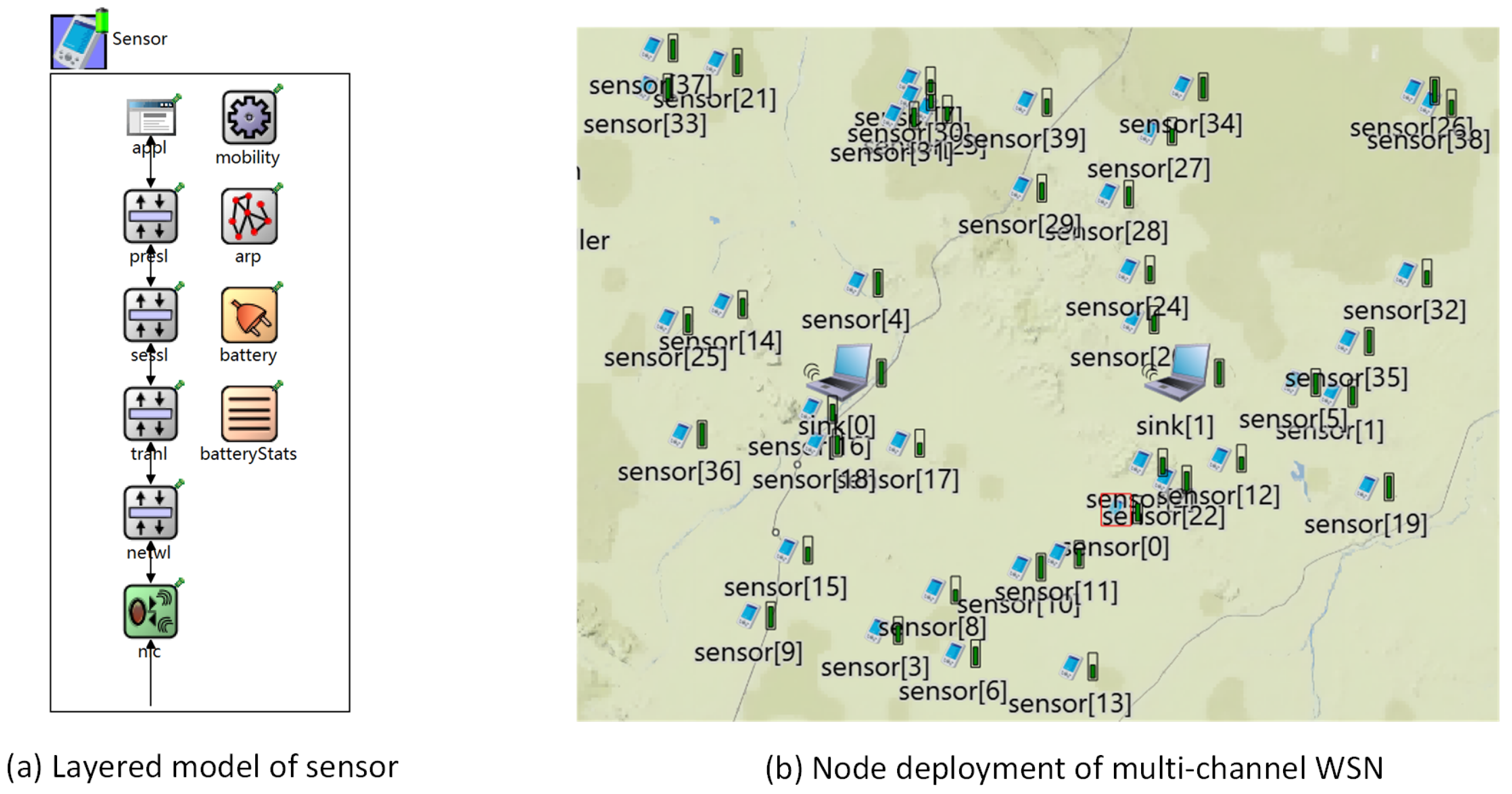
5.1. Simulation Setting

To simulate the realistic wireless network environment and reserve the concurrent execution characteristics of the distributed system, OMNeT++ is adopted to complete the task of performance evaluation. The model of the sensor node is constructed using the OSI model on this simulation platform, and the different functionalities of sensors are implemented on the corresponding logic layers. A visualization example of this layered sensor model is depicted in Figure 5a, where the “nic” layer contains both the physical and data link layer. In this model, the many-to-many data aggregation scheduling method is implemented as a MAC protocol. A periodic data collection event is implemented as the network application, which helps to make data aggregation produce a significant effect on data transmissions. The routing protocol at the network layer builds the routing structure to determine the upstream and downstream relationship of nodes. Sensor nodes are randomly deployed in simulation scenarios and the network always remains connected. A visualization example of node deployment on OMNeT++ is depicted in Figure 5b, where two sinks and 40 sources are located in a multi-channel WSN. By conducting a sufficient number of priori tests, there are some recommended settings for important system parameters. For example, $\alpha \in$ [0.05, 0.2], $\gamma \in$ [0.1, 0.3], $\sigma \in$ [2, 8].

The proposed method in this paper is named MDS-ML (Many-to-many Data aggregation Scheduling based on Multi-agent Learning for multi-channel WSN). As comparison targets of performance, three existing methods are selected. EESPG (Energy Efficient Scheduling in wireless sensor networks for Periodic data Gathering) [20] as a typical centralized method is adopted in simulation. Data Aggregation Scheduling method for multi-channel Duty cycle WSN called DASD [24] is implemented to support many-to-many communication mode, and it works in a centralized way. CDSM (Cluster-based distributed Data aggregation Scheduling algorithm with Multi-power and multi-channel) [26] using different transmission power and channels for intra-cluster and inter-cluster, respectively.

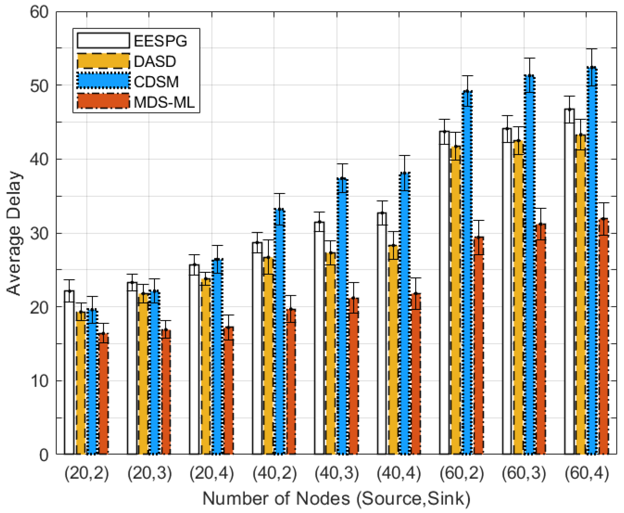
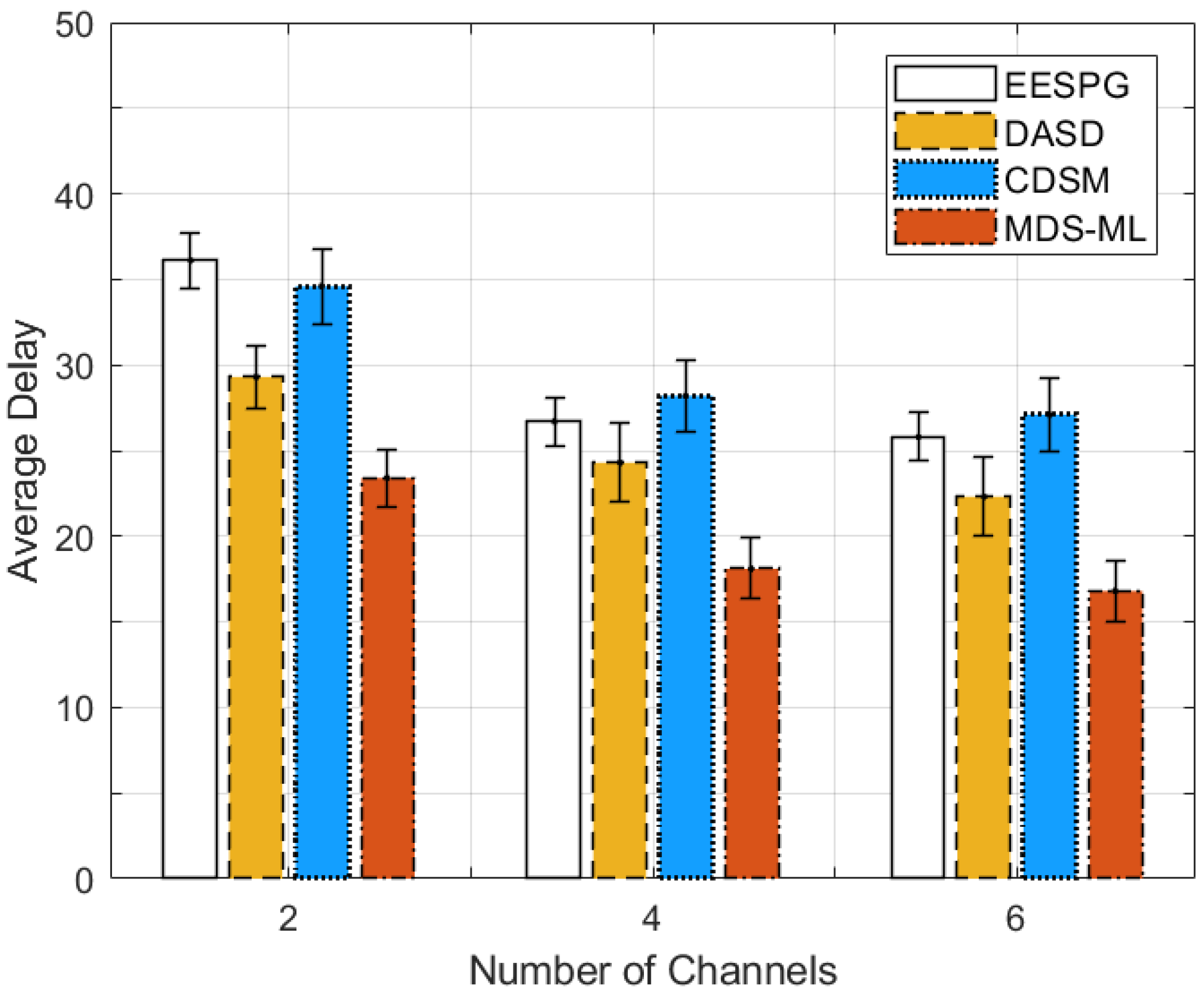
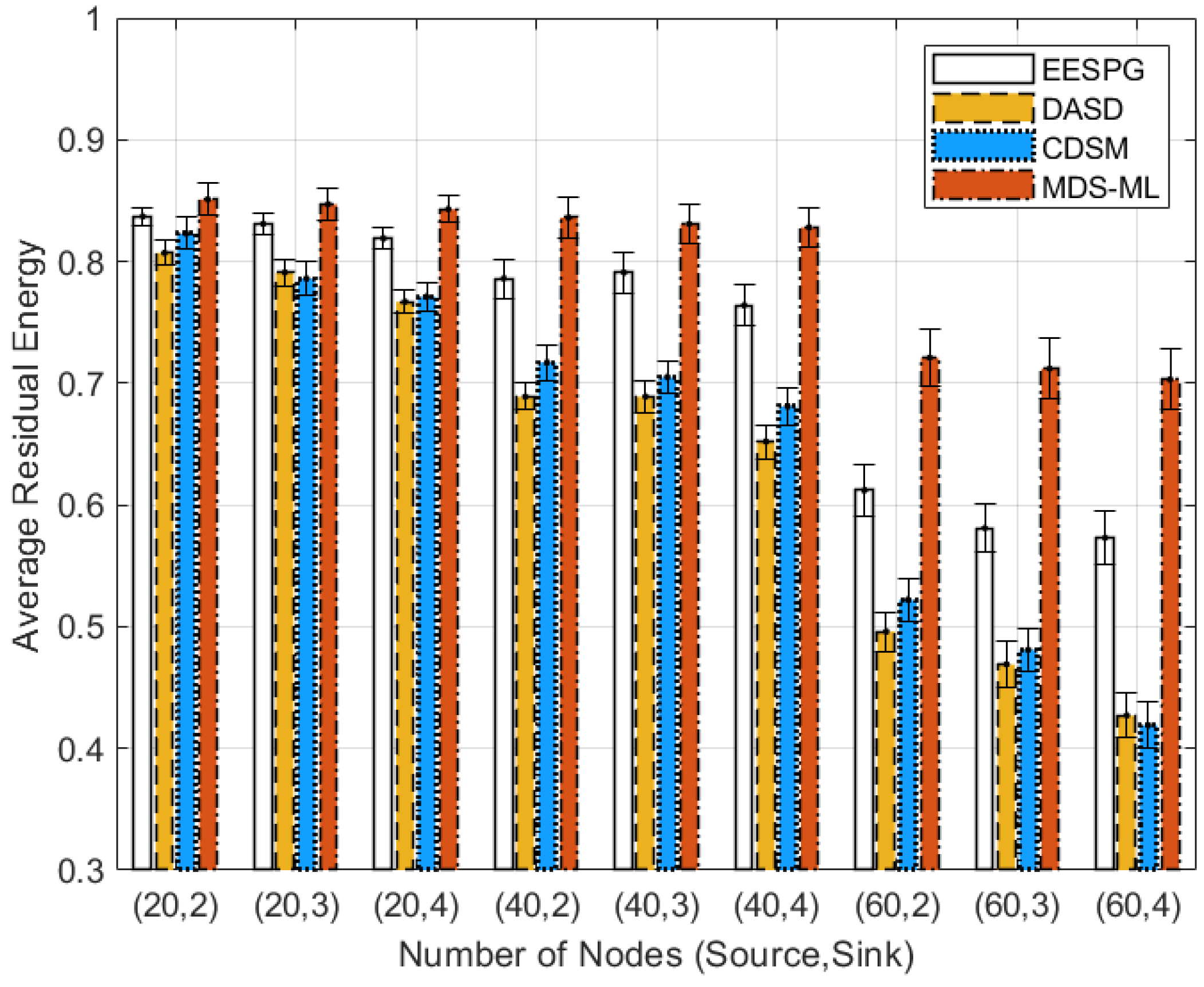
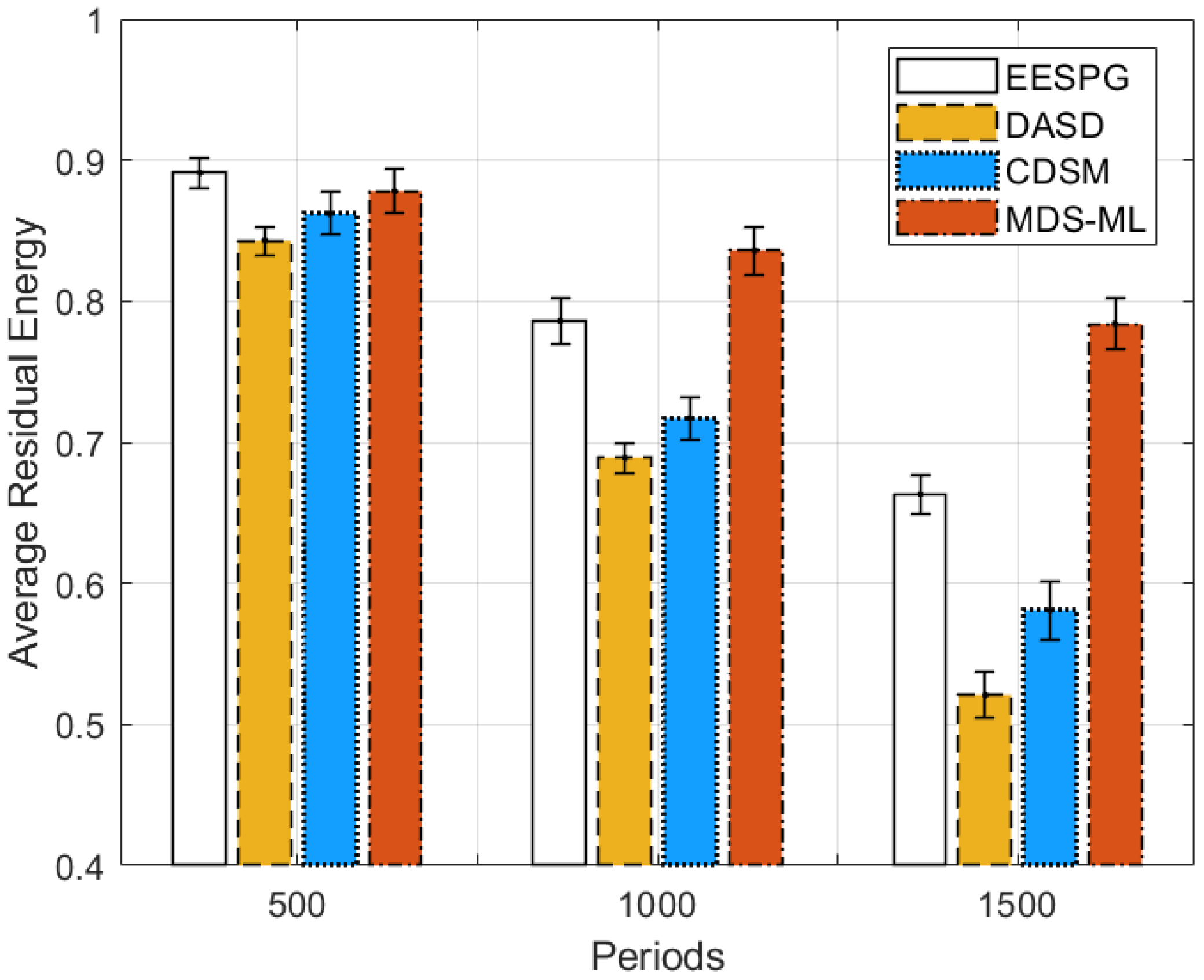
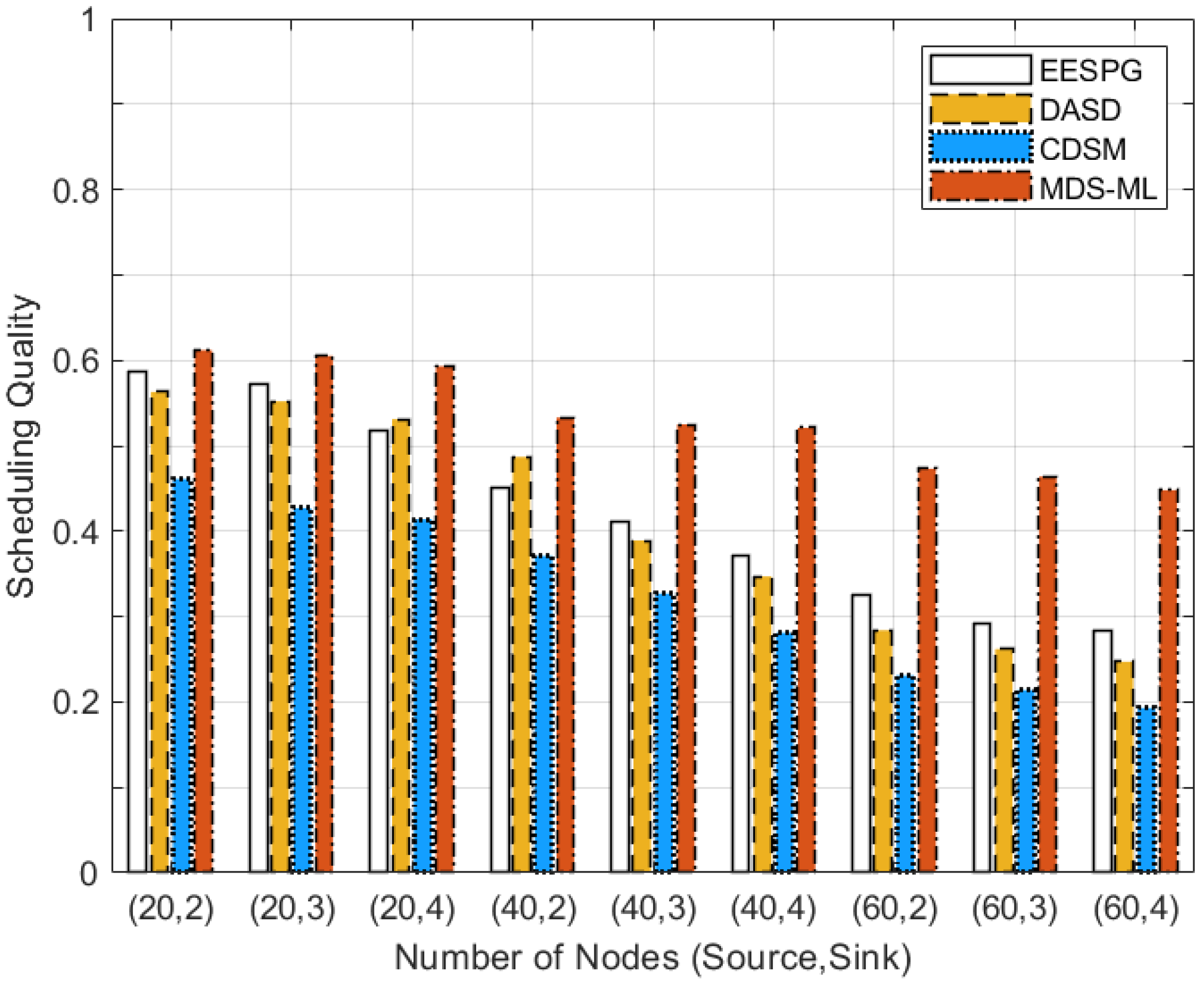
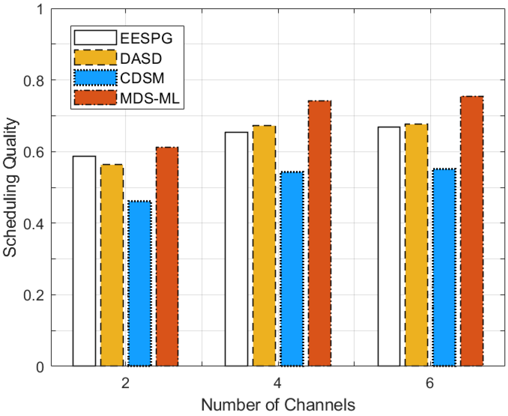
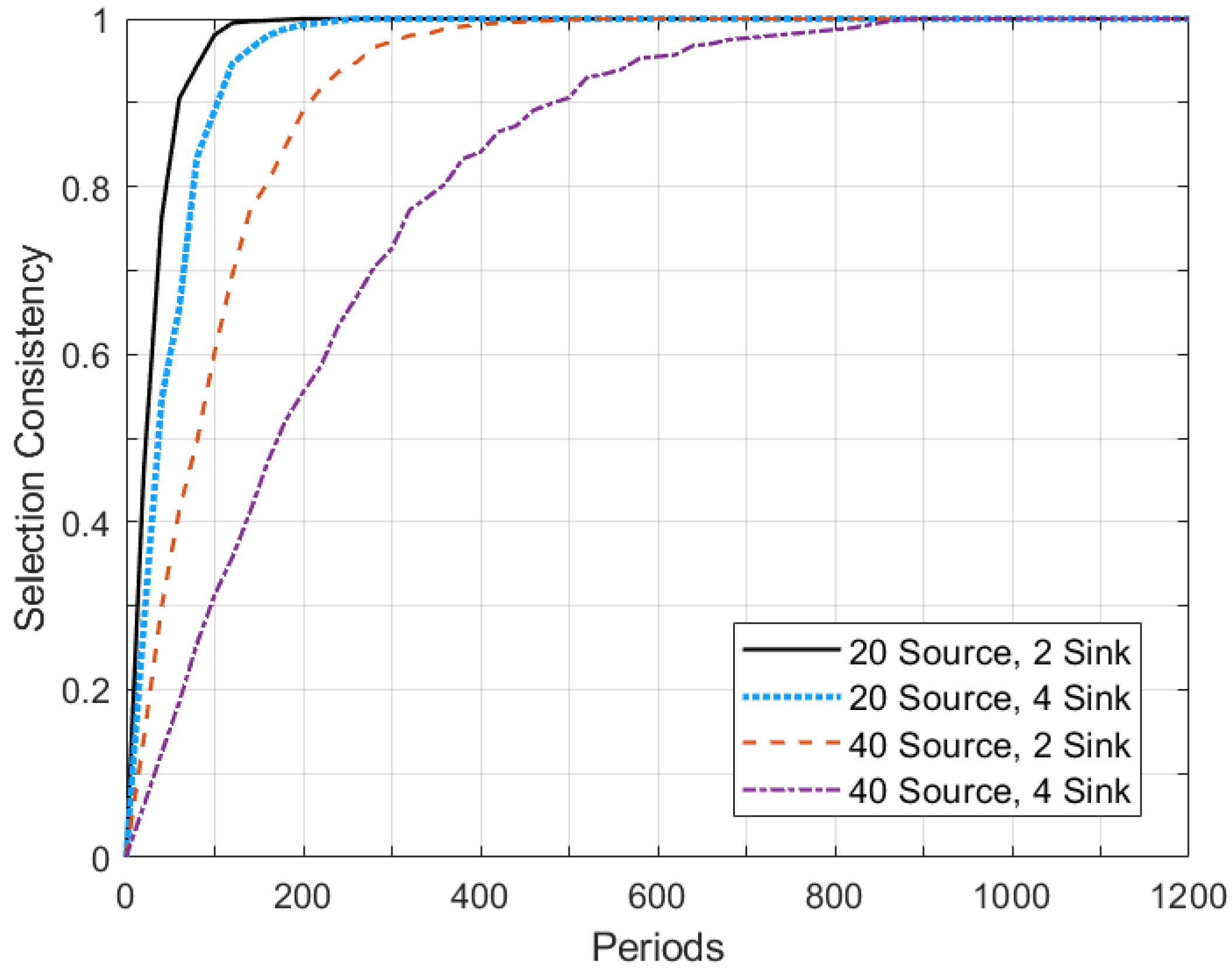
5.2. Performance Evaluation

The scheduling results are optimized using a multiple objectives function, such as communication delay and residual energy. Since one node only performs the scheduling operation once in one data collection period, the number of periods represents the number of time steps for a learning method. Figure 6 depicts the comparison results on an average delay, where the scenarios with the different number of nodes are displayed, and a tuple (source, sink) is used to denote the number of source nodes and sink nodes. If the source nodes or sink nodes increase, the average transmission delay will increase as well, because the network structure becomes more complex and the path of packet transmission usually becomes longer. EESPG, DASD and CDSM have higher values of average delay than MDS-ML. One possible reason is that these methods are originally designed for many-to-one data aggregation, and they have to transform some components to support many-to-many data aggregation. The gap between the compared methods and MDS-ML become more obvious along with the increase in nodes. When there are 60 source nodes and 4 sink nodes in the application scenario, MDS-ML has about a 36% lower delay than the second best performing DASD.

If more channels are available in network, all methods designed for a multi-channel WSN can obtain a lower delay; the related result can be found in Figure 7. When a wireless channel increases from 2 to 4, MDS-ML and EESPG decrease to 77% and 74% of their original value, respectively.

The impact of node number on the average residual energy is depicted in Figure 8. When there are 20 source nodes in a network, MDS-ML and EESPG have a similar performance; however, their difference becomes bigger along with the increase in source nodes. Especially for the scenario with 60 sources and 4 sinks, MDS-ML keeps its energy value about 22% higher than the value of EESPG. In addition, the increase in sink nodes has a relatively limited impact on the energy value of MDS-ML.

Figure 9 depicts the comparison result on average residual energy. DASD did not consider the reduction in energy consumption as a primary optimization objective, so it performs the worst among four methods, and its energy level drops quickly along with an increase in time. CDSM utilized different power and channel for different kinds of communication, but it also cannot obtain a satisfactory result due to its distributed nature. MDS-ML is hardly affected by the change in the number of periods, and its energy percentage is almost 1.5 times the energy percentage of DASD.

For the purpose of evaluating the comprehensive performance on multiple objectives, the weighted sum with normalized objective value is adopted. The value of weighted sum is named a scheduling quality, which represents the quality of an optimized scheduling result, and the comparison result on this metric with different numbers of nodes is depicted in Figure 10. More nodes involved in data transmission generally means the scheduling optimization becomes more complex, and it is harder to obtain a higher value of scheduling quality.MDS-ML always holds the best scheduling quality when comparing with the other three methods. In the scenario with 20 source nodes and 2 sink nodes, the quality of MDS-ML becomes almost 1.1 times larger than the quality of EESPG and DASD. When the number of sources and sinks become 60 and 4, the advantage increases to 1.5 times larger than the quality of EESPG and DASD, at most.

Figure 11 indicates the advancement made by our proposed method by comparing the scheduling quality with a different number of channels. CDSM always obtains the lowest value of scheduling quality. EESPG and DASD have a similar overall performance. In the scenario with four channels, the scheduling of MDS-ML is almost 1.4 times higher than CDSM. The benefits of increasing channels on scheduling quality becomes very little when the number of channels becomes 6.

In

Table 1. Impact of learning rate $\alpha$ on scheduling quality.

Periods	$\mathit{\alpha }$ = 0.05	$\mathit{\alpha }$ = 0.1	$\mathit{\alpha }$ = 0.2
500	0.13	0.39	0.73
1000	0.21	0.67	0.78
1500	0.37	0.85	0.81

, the impact of learning rate $\alpha$ on scheduling quality is presented. Along with the increase in time steps, the proposed method uses more steps to learn better policy and to obtain better quality. When $\alpha$ is small, the update rule keeps more of the original Q-value, so the learning speed in relatively slower. When $\alpha$ is set to 0.2, a scheduling with good quality is learned early, but it barely changs along with the increase in time steps. The most apparent variation with time steps happens when $\alpha =0.1$; the quality increases about 2.2 times.

In

Table 2. Impact of shrinking factor $\sigma$ on scheduling quality.

Periods	$\mathit{\sigma }$ = 2	$\mathit{\sigma }$ = 4	$\mathit{\sigma }$ = 6	$\mathit{\sigma }$ = 8
500	0.41	0.39	0.35	0.32
1000	0.55	0.67	0.58	0.48
1500	0.63	0.85	0.78	0.69

, the impact of shrinking factor $\sigma$ on scheduling quality is presented. The smaller value of shrinking factor leads to a higher probability of random action. Even though it may help to explore more different schedulings, it also may slow down the convergence speed due to too many random actions. An example can be found when $\sigma =2$: along with the increase in time steps, the quality only promotes about 1.5 times. The best performance on shrinking factor $\sigma$ is equal to 4 in these tests.

The convergence of scheduling result is an indispensable feature for learning-based methods, and a specific metric called selection consistency $SC$ is designed to observe the convergence of the proposed method. Let us assume the current period to be $t_c$; then, the selection consistency of an agent for recently observed periods $h_{rt}$ can be defined as follows:

$$SC\left(LS\right)=\frac{1}{h_{rt}-1}\sum _{i=t_c-h_{rt}+1}^{h_{rt}-1}\frac{\left|L{S}_i\bigcap L{S}_{i+1}\right|}{\left|L{S}_i\bigcup L{S}_{i+1}\right|}$$

(21)

Figure 12 depicts the result of selection consistency with different numbers of nodes; when the value is equal to 1, it means selection becomes stable and convergent. With the increase in nodes, MDS-ML takes more periods to reach consistency. When there 20 sources and 2 sinks, it only takes about 120 periods, and when there are 40 sources and 2 sinks in a network, it costs about 400 periods. This phenomenon is probably caused by the complexity of the scheduling problem. The more nodes represent more chance of conflicts, and arranging more working time slots and channels.

PLR (packet loss ratio) and PDR (packet delivery ratio), as two common performance metrics, are used to evaluate network throughput. By applying the proposed algorithm to the different network scenarios, the influence of the number of nodes on PLR and PDR can be further observed, and the corresponding result is depicted in Figure 13. In case of the fixed number of collection periods, the more complex network scenario with more nodes implies that the scheduling method spends more time to achieve convergence, so more packets will be lost due to the unsuccessful communications during the uncovergence stage. For example, PLR increases by about 4 times when the source nodes increase from 20 to 60 and the sink nodes increase from 2 to 4 in the simulation scenario. When there is 20 source nodes in the simulation scenarios, the change in sink number distinctly affects PLR and PDR. However, this tendency is gradually diminished if the number of source node reaches 60, where the gap among the scenarios with different sink numbers is only about $2.5\%$ at most.

5.3. Discussion of Simulation Results

According to the simulation results presented above, MDS-ML obtains better performance on transmission delay, energy consumption overall scheduling quality, and PLR and PDR. As this new scheduling method is directly designed for supporting many-to-many data aggregation in a multi-channel WSN, it also considers multiple optimization objectives. Thanks to the feature of continuous learning, this new method can obtain good performance for data transmission. CDSM as a distributed scheduling method lacks the optimization capability for the global network; then, it achieves the relatively poor performance. Although EESPG and DASD have good performance as well, the construction and maintenance of a virtual tree structure still increases the additional network overhead, because the exchanges of extra control packets among nodes are inevitable, and they target implementing the many-to-one data aggregation scheduling for multiple channels. When these scheduling methods are compulsorily applied into the multi-sink scenarios, concurrent and independent scheduling operations toward different sinks have to be executed, and these operations without cooperation lead to higher costs in the network. The performance advantage of the new method is more obvious when there are more source nodes and sink nodes in simulation scenarios. Since the network structure becomes more complex, it is more difficult to find the optimal scheduling set.

6. Conclusions

To handle the many-to-one data aggregation scheduling problem for a multi-channel WSN, a cooperative multi-agent learning-based scheduling method is proposed in this paper. The optimization goal of scheduling is formulated and analysed, firstly. According to the characteristics of many-to-many data aggregation scheduling, the scheduling process is mapped to a decentralized partially observable Markov decision model. The cooperative multi-agent learning is implanted into a many-to-many data aggregation scheduling procedure. Nodes within one hop distance establish a group, which is a basic cooperative unit to learn the optimal policy. Finally, performance experiments are conducted on a discrete event simulator, and the simulation results validate the advantage of the proposed method on common metrics. In future work, a more detailed system model which is closer to the realistic communication environment should be considered for the proposed scheduling method. In this new model, the channel fading problem will be effectively handled, the communication security will be guaranteed, the malicious and selfish nodes will be detected and prevented.

References

1. Jamshed, M.A.; Ali, K.; Abbasi, Q.; Imran, M.A. Challenges, Applications and Future of Wireless Sensors in Internet of Things: A Review. IEEE Sens. J. 2022, 22, 5482–5494. [Google Scholar] [CrossRef]
2. Mohamed, S. Abdalzaher, Lotfy Samy, Osamu Muta, Non-zero-sum game-based trust model to enhance wireless sensor networks security for IoT application. IET Wirel. Sens. Syst. 2019, 9, 218–226. [Google Scholar]
3. Ballard, Z.; Brown, C.; Madni, A.M.; Ozcan, A. Machine learning and computation-enabled intelligent sensor design. Nat. Mach. Intell. 2021, 3, 556–565. [Google Scholar] [CrossRef]
4. Izhar; Wang, X.; Xu, W.; Tavakkoli, H.; Lee, Y.K. Integrated Predicted Mean Vote Sensing System Using MEMS Multi-Sensors for Smart HVAC Systems. IEEE Sens. J. 2021, 21, 8400–8410. [Google Scholar] [CrossRef]
5. Shi, W.; Jie, C.; Quan, Z.; Li, Y.; Xu, L. Edge computing: Vision and challenges. IEEE Internet Things J. 2016, 3, 637–646. [Google Scholar] [CrossRef]
6. El-Sayed, H.; Sankar, S.; Prasad, M.; Puthal, D.; Gupta, A.; Mohanty, M.; Lin, C.-T. Edge of Things: The Big Picture on the Integration of Edge, IoT and the Cloud in a Distributed Computing Environment. IEEE Access 2018, 6, 1706–1717. [Google Scholar] [CrossRef]
7. Gholami, N.; Moghim, N.; Ghazvini, M.; Haghani, S. Utilizing Non-Orthogonal Multiple Access for Both Latency and Energy Efficiency Improvement in TSCH-Based WSNs. IEEE Access 2022, 10, 28922–28937. [Google Scholar] [CrossRef]
8. Cheng, L.; Kong, L.; Gu, Y.; Niu, J.; Zhu, T.; Liu, C.; Mumtaz, S.; He, T. Collision-Free Dynamic Convergecast in Low-Duty-Cycle Wireless Sensor Networks. IEEE Trans. Wirel. Commun. (TWC) 2022, 21, 1665–1680. [Google Scholar] [CrossRef]
9. Boubiche, S.; Boubiche, D.E.; Bilami, A.; Toral-Cruz, H. Big Data Challenges and Data Aggregation Strategies in Wireless Sensor Networks. IEEE Access 2018, 6, 20558–20571. [Google Scholar] [CrossRef]
10. Saginbekov, S.; Jhumka, A. Many-to-many data aggregation scheduling in wireless sensor networks with two sinks. Comput. Netw. 2017, 123, 184–199. [Google Scholar] [CrossRef] [Green Version]
11. Wang, C.; Zhang, Y.; Song, W.-Z. A new data aggregation technique in multi-sink wireless sensor networks. In Proceedings of the International Conference on Smart Computing Workshops, Hong Kong, China, 5 November 2014; pp. 99–104. [Google Scholar]
12. Huang, Y.; Zhao, C.; Tang, B.; Fu, H. Beacon Synchronization-Based Multi-Channel with Dynamic Time Slot Assignment Method of WSNs for Mechanical Vibration Monitoring. IEEE Sens. J. 2022, 22, 13659–13667. [Google Scholar]
13. Terauchi, T.; Suto, K.; Wakaiki, M. Harvest-Then-Transmit-Based TDMA Protocol with Statistical Channel State Information for Wireless Powered Sensor Networks. In Proceedings of the 93rd IEEE Vehicular Technology Conference (VTC), Helsinki, Finland, 25–28 April 2021; pp. 1–5. [Google Scholar]
14. Abdalzaher, M.S.; Muta, O. Employing Game Theory and TDMA Protocol to Enhance Security and Manage Power Consumption in WSNs-Based Cognitive Radio. IEEE Access 2019, 7, 132923–132936. [Google Scholar] [CrossRef]
15. Abdalzaher, M.S.; Muta, O. A Game-Theoretic Approach for Enhancing Security and Data Trustworthiness in IoT Applications. IEEE Internet Things J. 2020, 7, 11250–11261. [Google Scholar] [CrossRef]
16. Elwekeil, M.; Abdalzaher, M.S.; Seddik, K. Prolonging smart grid network lifetime through optimising number of sensor nodes and packet length. IET Commun. 2019, 13, 2478–2484. [Google Scholar] [CrossRef]
17. Liu, D.; Wu, X.; Cao, Z.; Liu, M.; Li, Y.; Hou, M. CD-MAC: A contention detectable MAC for low duty-cycled wireless sensor networks. In Proceedings of the 12th Annual IEEE International Conference on Sensing, Communication, and Networking (SECON), Seattle, WA, USA, 22–25 June 2015; pp. 37–45. [Google Scholar]
18. Nguyen, N.-T.; Liu, B.-H.; Pham, V.-T.; Liou, T.-Y. An Efficient Minimum-Latency Collision-Free Scheduling Algorithm for Data Aggregation in Wireless Sensor Networks. IEEE Syst. J. 2018, 12, 2214–2225. [Google Scholar] [CrossRef]
19. Kang, B.; Nguyen, P.K.H.; Zalyubovskiy, V.; Choo, H. A Distributed Delay-Efficient Data Aggregation Scheduling for Duty-Cycled WSNs. IEEE Sens. J. 2017, 17, 3422–3437. [Google Scholar] [CrossRef]
20. Kumar, S.; Kim, H. Energy Efficient Scheduling in Wireless Sensor Networks for Periodic Data Gathering. IEEE Access 2019, 7, 11410–11426. [Google Scholar] [CrossRef]
21. Ma, J.; Lou, W.; Li, X. Contiguous Link Scheduling for Data Aggregation in Wireless Sensor Networks. IEEE Trans. Parallel Distrib. Syst. 2014, 25, 1691–1701. [Google Scholar] [CrossRef] [Green Version]
22. Yao, B.; Gao, H.; Chen, Q.; Li, J. Energy-Adaptive and Bottleneck-Aware Many-to-Many Communication Scheduling for Battery-Free WSNs. IEEE Internet Things J. 2021, 8, 8514–8529. [Google Scholar] [CrossRef]
23. Bagaa, M.; Younis, M.; Ksentini, A.; Badache, N. Reliable Multi-channel Scheduling for timely dissemination of Aggregated data in Wireless Sensor Networks. J. Netw. Comput. Appl. 2014, 46, 293–304. [Google Scholar] [CrossRef]
24. Jiao, X.; Lou, W.; Feng, X.; Wang, X.; Yang, L.; Chen, G. Delay Efficient Data Aggregation Scheduling in Multi-channel Duty-Cycled WSNs. In Proceedings of the IEEE 15th International Conference on Mobile Ad Hoc and Sensor Systems (MASS), Chengdu, China, 9–12 October 2018; pp. 326–334. [Google Scholar]
25. Lu, Y.; Zhang, T.; He, E.; Ioan-Sorin, C. Self-learning-based data aggregation scheduling policy in wireless sensor networks. J. Sens. 2018, 2018, 9647593. [Google Scholar] [CrossRef] [Green Version]
26. Ren, M.; Li, J.; Guo, L.; Cai, Z. Distributed Data Aggregation Scheduling in Multi-channel and Multi-power Wireless Sensor Networks. IEEE Access 2017, 5, 27887–27896. [Google Scholar] [CrossRef]
27. Lee, J.; Jeong, W. Multi-channel TDMA link scheduling for wireless multi-hop sensor networks. In Proceedings of the International Conference on Information and Communication Technology Convergence (ICTC), Jeju, Korea, 28–30 October 2015; pp. 630–635. [Google Scholar]
28. Yu, B.; Li, J. Minimum-time aggregation scheduling in multi-sink sensor networks. In Proceedings of the 8th Annual IEEE Communications Society Conference on Sensor, Mesh and Ad Hoc Communications and Networks, Jeju, Korea, 28–30 October 2011; pp. 422–430. [Google Scholar]
29. Mottola, L.; Picco, G.P. MUSTER: Adaptive Energy-Aware Multisink Routing in Wireless Sensor Networks. IEEE Trans. Mob. Comput. 2011, 10, 1694–1709. [Google Scholar] [CrossRef] [Green Version]
30. Yu, J.; Yu, W.; Gu, J. Online Vehicle Routing with Neural Combinatorial Optimization and Deep Reinforcement Learning. IEEE Trans. Intell. Transp. Syst. 2019, 20, 3806–3817. [Google Scholar] [CrossRef]
31. Amato, C.; Konidaris, G.; Kaelbling, L.P.; How, J.P. Modeling and planning with macro-actions in Decentralized POMDPs. J. Artif. Intell. Res. 2019, 64, 817–859. [Google Scholar] [CrossRef] [PubMed] [Green Version]
32. Zhang, C.; Lesser, V.R. Coordinated Multi-Agent Reinforcement Learning in Networked Distributed POMDPs. In Proceedings of the Twenty-Fifth AAAI Conference on Artificial Intelligence (AAAI), San Francisco, CA, USA, 7–11 August 2011; pp. 7–11. [Google Scholar]
33. Farinelli, A.; Rogers, A.; Jennings, N.R. Agent-based decentralised coordination for sensor networks using the max-sum algorithm. Auton. Agents -Multi-Agent Syst. 2014, 28, 337–380. [Google Scholar] [CrossRef]
34. Jin, C.; Allen-Zhu, Z.; Bubeck, S.; Jordan, M.I. Is Q-learning provably efficient. In Proceedings of the 32nd International Conference on Neural Information Processing Systems (NIPS’18), Red Hook, NY, USA, 3–8 December 2018; pp. 4868–4878. [Google Scholar]
Figure 1. Example of many-to-many data aggregation scheduling in WSN.
Electronics 11 03356 g001
Figure 2. Example of communication conflicts.
Electronics 11 03356 g002
Figure 3. Example of many-to-many data aggregation scheduling on a node.
Electronics 11 03356 g003
Figure 4. Example of group cooperation.
Electronics 11 03356 g004
Figure 5. Visualization example of network model on OMNeT++.
Electronics 11 03356 g005
Figure 6. Average delay with different number of nodes.
Electronics 11 03356 g006
Figure 7. Average delay with different number of channels.
Electronics 11 03356 g007
Figure 8. Average residual energy with different number of nodes.
Electronics 11 03356 g008
Figure 9. Average residual energy with different number of periods.
Electronics 11 03356 g009
Figure 10. Comparison of scheduling quality with different number of nodes.
Electronics 11 03356 g010
Figure 11. Comparison of scheduling quality with different number of channels.
Electronics 11 03356 g011
Figure 12. Selection consistency.
Electronics 11 03356 g012
Figure 13. Average PLR and PDR with different nodes.
Electronics 11 03356 g013