1. Introduction
During signal transmission, according to the relationship between the sender and the receiver, the communication process can be divided into two modes: cooperative and non-cooperative. In the cooperation mode, the relevant parameters of the signal are known to both the receiving and sending terminals; in the noncooperative mode, the parameters related to the signal transmission at the receiving end are only partially known or completely unknown. The modulation recognition technology mainly works in the non-cooperative mode to identify the modulation mode and its parameters of the signal to be detected, such as carrier frequency, symbol rate, etc.
In the field of military communications, information warfare has become a key factor in the victory of a war. Mastering more information in a war often means taking a greater initiative. Modulation recognition technology, originated from military communication, is the early foundation and necessary condition for electronic reconnaissance, target detection, communication warning, monitoring and other activities. In military information warfare, modulation recognition technology can be used to intercept unknown wireless signals, decode them, extract information, and obtain the communication content of the target; The jamming parameters can also be set according to the identified modulation information to generate corresponding jamming signals, so as to realize the jamming of enemy wireless signals. Therefore, an efficient, fast and accurate modulation recognition system is of great significance for occupying the information commanding heights in modern information warfare.
Signal modulation recognition technology mainly refers to the technology of distinguishing the modulation mode used by the modulation signal and estimating the modulation related parameters in the absence of relevant prior information [
1]. Modulation recognition technology has always been an important basic technology in military and civil fields such as electronic reconnaissance and radio monitoring. The traditional modulation recognition technology mainly uses the signal time domain waveform and its transform domain characteristics to identify and judge. The recognition process depends on the subjective experience of algorithm designers, which has low work efficiency, high labor cost and poor universality of the algorithm. Nowadays, with the improvement of hardware computing power and the wide application of artificial intelligence algorithm theory, artificial intelligence related algorithms are applied to the field of signal modulation recognition with high recognition rate, high speed and good applicability, which will have a very broad development prospect and application space in military and civil fields.
Modulation recognition is the process of determining the modulation mode of digital signal by means of signal correlation feature extraction. It is not only a part of modulation recognition, but also the basis of subsequent operations such as signal demodulation, interpretation and information extraction. Modulation recognition is mainly divided into the traditional methods (such as statistical mode, decision theory, neural network, wavelet transform and so on) and deep learning methods based on convolutional natural network [
2]. Liu et al. combines the traditional method with the feature of power spectrum sidelobe attenuation to recognize the 5G signal [
3]. Izhou Gep et al. proposed a method which combines the method of cyclic spectrum with high-order cumulant to perform the modulation recognition of UWA communication to improve rate recognition of underwater signals at low SNR [
4].
Most traditional method based on artificial designed features to recognition, the ability of this kind of algorithm is limited. The modulation recognition algorithm based on deep learning uses the ability of network model to extract the characteristics of graphic data, recognizes the digital signal through autonomous learning, and can also be recognized under the condition of less a priori information. At the same time, it can reduce the dependence on the subjective experience of algorithm designers. Ya Liu et al. first tried to use graph convolution neural network to solve the problem of high algorithm complexity, which can effectively reduce the algorithm complexity of deep learning network [
5]. Dechun Sun et al. proposed a modulation recognition algorithm based on VGG convolutional neural network, aiming at the difficulty of feature extraction of traditional algorithms under low SNR. This algorithm makes up for the shortage of manual feature extraction, converts the sampled data of communication signal into gray image, and trains the model and classifies it through VGG network [
6]. In view of the characteristics that traditional recognition algorithms mostly rely on manual design, which leads to the application limitations of the algorithm, Zhang Tingting et al. proposed a modulation recognition algorithm based on the Gate Recurrent Unit (GRU), which uses a multi-layer bidirectional GRU network structure to improve the feature representation ability [
7]. Ke Bu et al. introduced Adversarial Transfer Learning Architecture (ATLA) into deep learning, combined adversarial training with knowledge transfer, and reduced the sample size of training set [
8]. In order to solve the problem of low recognition rate under low SNR, Fugang Liu et al. optimized on the basis of Long Short-Term Memory (LSTM) networks [
9]. This method first extracts the characteristics of the signal, such as advanced cumulants, and then sends them to the parallel network composed of convolutional neural network and GRU for recognition. Zhang et al. proposed a framework called Attention Relation Network (ARN) which introduced channel and spatial attention, respectively to learn a more effective feature representation of support samples [
10]. Wu et al. pointed out that most existing automatic modulation recognition (AMR) algorithm highly depended on the feature of data, so they introduced the LSTM as the classifier into neural network to improve the robustness [
11]. Yang et al. proposed an algorithm based on AlexNet to increase the rate of recognition [
12]. High-order Quadrature Amplitude Modulation (QAM) has problem that the performance severely degraded in multipath fading channels, Xuefei et al. proposed an algorithm that combines a blind equalization module and ResNet [
13].
In addition, machine learning has a good performance in modulation recognition. Because of the characters of the algorithm itself, deep learning also has some problems such as having a complex learning process in neural networks, learning results cannot be corrected, training is time-consuming, model correctness verification is complex and cumbersome. Chou et al. used K-means cluster algorithm to contain the feature of the signal constellation to reduce the complexity of the algorithm [
14]. H. TAYAKOUT et al. used a simplified Distributed Space-Time Block Coding (D-STBC) scheme for a three-node cooperative network system incorporating, which addresses the problem of semi-blind automatic digital modulation recognition for wireless relaying network [
15]. Liu Wang et al. proposed a clustering algorithm to automatically choose the center of the constellation according to the number of center points [
16]. Punith et al. proposed a new algorithm to distinguish between 6 digital modulation schemes by using adaptive threshold methods [
17].
Aiming at the low recognition accuracy of traditional modulation recognition methods under low SNR conditions, a modulation recognition algorithm model based on the characteristics of digital signal constellation is proposed. The algorithm model first converts the signal into the form of constellation diagram, uses density clustering algorithm for noise reduction, and inputs the features extracted by KADPC algorithm into multi-level SVM classifier to obtain modulation recognition results. This method reduces the complexity of feature extraction and the cost of classification. Compared with traditional modulation recognition methods, this method can improve the recognition performance of several common types of digital modulation signals. The rest of this paper is organized as follows.
Section 2 briefly introduces the proposed methods relevant and improvements in this paper. The experimental results and analysis are given in
Section 3.
Section 4 summarizes the conclusions and future work.
2. Algorithm Design
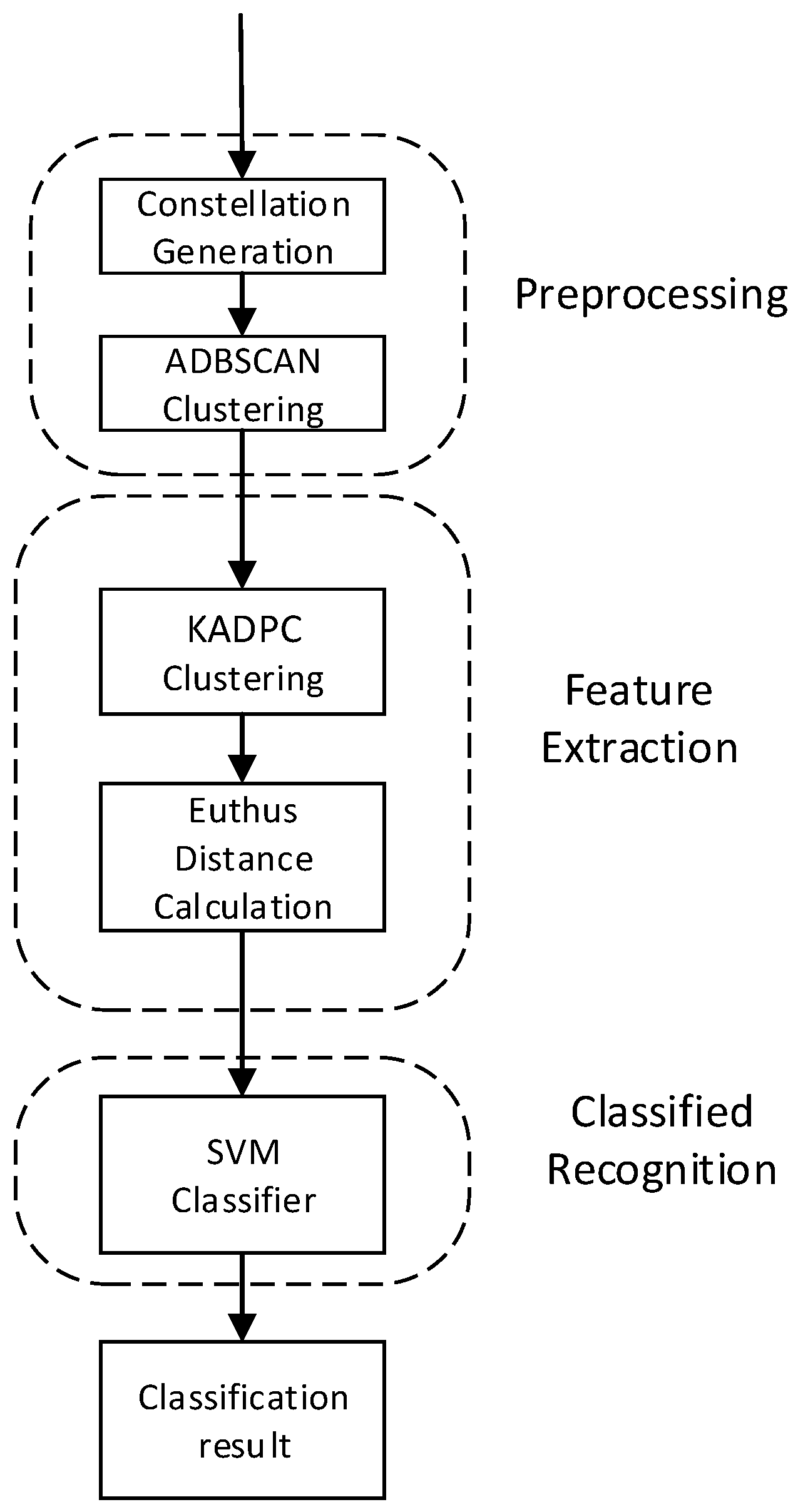
The proposed algorithm including three parts: preprocessing, feature extraction, and modulation type recognition. The block diagram of the modulation recognition algorithm is shown in
Figure 1. The preprocessing part transforms the signal to be detected into the form of constellation, uses ADBSCAN to reduce noise, and obtains the noise reduced constellation. In the feature extraction part, K-means is improved by using density peak clustering. Clustering is performed on the constellation after noise reduction and the eigenvalues are calculated to input into the SVM classifier for classification. In the classification part, multiple SVM cascades are used to form a multi-level classifier. The extracted eigenvalues are classified to obtain the recognition results of digital signal modulation.
2.1. Denoising Processing Based on ADBSCAN
In digital communication, constellation diagram is a more visual and direct method to represent the signal to be detected, which is generated by orthogonal modulation The received signal is divided into two channels after receiving the signal and multiplies by two carries with a phase difference /2, then goes through a low-pass filter. Then, two separate components the in-phase component and the quadrature component are obtained. Constellation diagram consists of two coordinate axes, the horizontal X-axis is relevant to the in-phase component, the vertical Y-axis is relevant to the quadrature component, each point in the diagram contains four information. The projection in X-axis defines the peak amplitude of in-phase component, the projection in Y-axis defines the peak amplitude of quadrature component, the length of the line from the point to the origin is the peak amplitude of the signal element, the angle between the line and the X-axis is the phase of the signal element. Because of the noise interference, it is hard to recognize the modulation of the constellation diagram, so ADBSCAN clustering algorithm is used into reducing noise in preprocessing parts.
DBSCAN (Density-Based Spatial Clustering of Applications with Noise) clustering algorithm, a kind of fast-clustering algorithm [
17], has a fast and good affection in processing the noise [
18]. The algorithm uses threshold density as the classify standard based on a fact that one clustering algorithm can be determined by any core object of the sample [
19], meanwhile the number of the clusters can be determined by the tightness of the sample distribution. Through classifying connected samples into one cluster, a cluster category is obtained. The final results of all categories are obtained by dividing all closed connected samples into different categories.
Consuming the sample set D = (), describes the neighborhood distance threshold of a sample, Minpts describes the threshold of the number of samples in the neighborhood where the distance of a sample is , the parameter definition of ADBSCAN clustering algorithm is defined as follows:
1.
neighborhood: For
, the neighborhood whose distance from
is not greater than
is defined as
:
2. Core object: For
, if the
corresponding to the neighborhood contains at least
Minpts samples, then the core object is defined as follows:
3. Directly density-reachable: If is located in the neighborhood of , and is the core object, then is said to be direct by the density of .
4. Density-reachable: For and , if there are sample sequences , satisfying = , = , and is directly reached by the density of , then is said to be reachable by the density of . In other words, the density can be reached to meet the transitivity. At this time, the transmitted samples in the sequence are all core objects, because only core objects can directly reach the density of other samples. Note that the density is reachable and does not satisfy the symmetry, this can be derived from the direct asymmetry of the density.
5. Density-connected: For and , if there is a core constellation sample , so that both and are reachable by the density of , then and are called density connected. Note that the density connection relationship satisfies symmetry.
According to the principle of ADBSCAN clustering, the category or cluster of the largest connectable sample set is found from the density reachable relationship as the final result. If there is only one core object in an ADBSCAN cluster, all non-core object constellation points in the cluster are in the
neighborhood of the constellation point; if there are multiple core objects, there is a density reachable relationship between any two core objects. Because ADBSCAN does not need to determine the number of clusters during clustering, it can denoise the signal constellation during digital signal preprocessing. The specific steps of ADBSCAN clustering algorithm are shown in Algorithm 1.
| Algorithm 1 ADBSCAN clustering algorithm |
INPUT: Constellation sample coordinate set D =
)
OUTPUT: Clustering results
- Step1:
and Minpts are automatically determined by calculating the distance between constellation sample points. - Step2:
Initialize the core object collection , cluster number unvisited sample set and cluster interval . - Step3:
For follow the steps below to find all core objects: - (a)
Find the neighborhood sub-sample set of the sample through the distance measurement method. - (b)
If the number of samples in the sub-sample set satisfies , add sample to the core object sample set: .
- Step4:
If the core object set , the algorithm ends, otherwise, go to step 5. - Step5:
In the core object set , randomly select a core object , initialize the current cluster core object queue , the category number and the current cluster sample set , update the unvisited samples set . - Step6:
If the current cluster core object queue , the current cluster has been generated, update the cluster division and the core object set go to step 4. Otherwise, update the core object set . - Step7:
Take a core object from the current cluster core object queue , find all neighborhood subsample sets through the neighborhood distance threshold , let , update the current cluster sample set , the unvisited sample set , and , go to step 6.
The output result is Cluster division
|
2.2. Feature Extraction
In this paper, K-means combined with auto DPC (KADPC) algorithm is used for feature extraction. K-means clustering algorithm, a traditional clustering based on distance, according to the distance between the sample points and the cluster center to cluster data. As the most classical unsupervised clustering algorithm, the main purpose of K-means is to divide all the samples to K clusters, make the sample similarity between the same class is as high as possible, and the similarity between different categories is as small as possible. Points on the constellation map that are closely distributed around the cluster center can well be clustered.
DPC is a fast-clustering algorithm, based on density peaks, according to the density distribution of sample points to determine the clustering result. DPC algorithm is greatly affected by the local density, when a sample is classified incorrectly, the remaining points are greatly affected, the classification result is easy to cause errors. K-means algorithm selects the initial clustering center randomly when clustering the constellation diagram. Thus, the clustering result has greater randomness, and the number of clustering centers needs to be determined before clustering. In modulation recognition, the number of cluster centers cannot be known in advance. Therefore, in this paper, the idea of DPC algorithm is used for improving the K-means algorithm. According to the distribution of points in the constellation diagram, find the points with the highest density as cluster centers, thereby reducing the number of iterations of K-means clustering and improving the clustering effect.
KADPC is an auto clustering algorithm combined with K-means and DPC clustering algorithm, whose parameters are defined as follows:
1. Cutoff distance
: let the cutoff distance gradually increase from zero, and find the cutoff distance that makes the entropy
H reach the minimum
2. Local density
: Define the local density of point
in the constellation diagram with local density
as:
3. High local density point distance
:
where
is the distance between any two constellation point
and
,
is the decision function. The specific steps of KADPC clustering algorithm are shown in Algorithm 2.
| Algorithm 2 KADPC clustering algorithm |
INPUT: Sample set D = )
OUTPUT: Eigenvalues - Step1:
Obtain the truncation distance by increasing the truncation distance from zero to the distance that minimizes the entropy H. - Step2:
According to the truncation distance , the local density value of constellation points in the constellation diagram is calculated, and the distance between other constellation points and high local density constellation points is calculated. - Step3:
Use the value of the calculated local density and the distance of high local density point to make a two-dimensional decision diagram to select the cluster center of the data sample, that is, select the point with the larger and as the cluster center: - Step4:
Select K cluster centers and perform K-means clustering on the selected K cluster centers: - Step5:
Calculate the sum of the Euclidean distances from the points in the K cluster to the centers of this cluster, find the average value of the sum of distances :
- Step6:
Normalize , and define unit Euclidean distance as the eigenvalue
|
In modulation recognition, the modulation method of the signal cannot be known, and the number of cluster centers cannot be determined. The number of cluster centers obtained by the existing modulation method is limited, and the number of cluster centers can be set multiple times, Classify and recognize the obtained set of feature values as the features of the signal, that is, the value of K can be set to 2, 4, 8, 16, 32, 64, and the corresponding feature values obtained are T2, T4, T8, T16, T32, T64.
2.3. Modulation Recognition Based on Multi-SVM
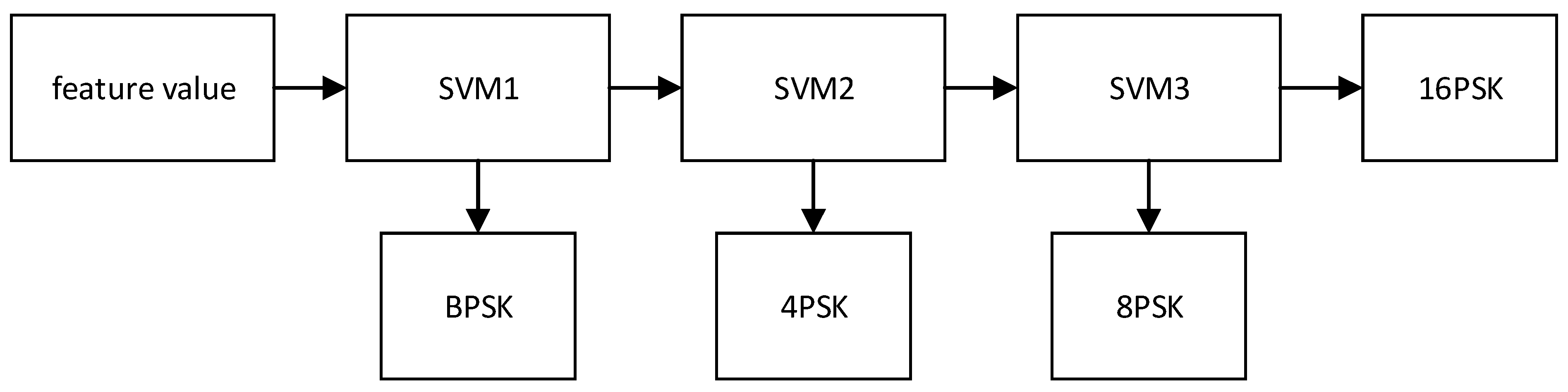
The basic SVM model is a linear classifier with the largest interval defined in the feature space. Since the use of the kernel function method overcomes the curse of dimensionality and the problem of non-linear separability, there is no increase in computational complexity when mapping to a high-dimensional space. The SVM classification algorithm was originally only used to solve two classification problem, and lacked the ability to deal with multi-classification problems. Due to the wide variety of modulation methods, in order to reduce the number of SVM classifiers, one-versus-rest (OVR) SVM is used in this paper. Take BPSK, 4PSK, 8PSK and 16PSK as classification targets to realize multi classification, three SVM classifiers are used to form a multi-classifier as shown in
Figure 2, for each classifier is composed of the eigenvalues of the same signal under different SNR.
In the data training process, the training of each classifier is composed of the eigenvalues of the same signal under different SNRs, thus reducing the amount of parameter training, as shown in Equation (8).
3. Experimental Results and Analysis
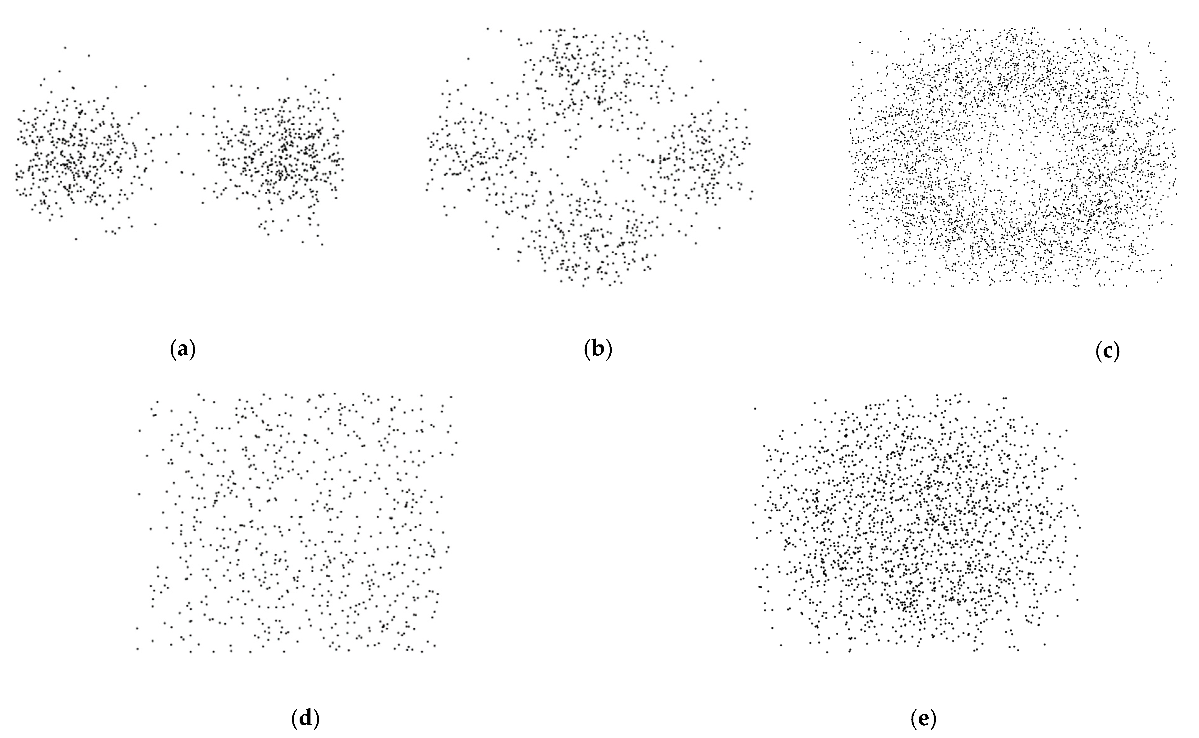
In order to verify the feasibility of the algorithm, MATLAB is used in this paper to simulate Phase Shift Keying (PSK) and Quadrature Amplitude Modulation (QAM) signal to obtain BPSK, QPSK, 8PSK, 16QAM, 32QAM at different SNRs.
Figure 3 are the constellation diagrams of the five signals at SNR = 6 dB. The symbol rate of each signal is 1200 B/s, the number of symbols is 4000, the carrier frequency is 4800 Hz and the sampling frequency is 16 × 4800 Hz. Gaussian white noise is added to simulate the transmission of all signals on the Gaussian channel.
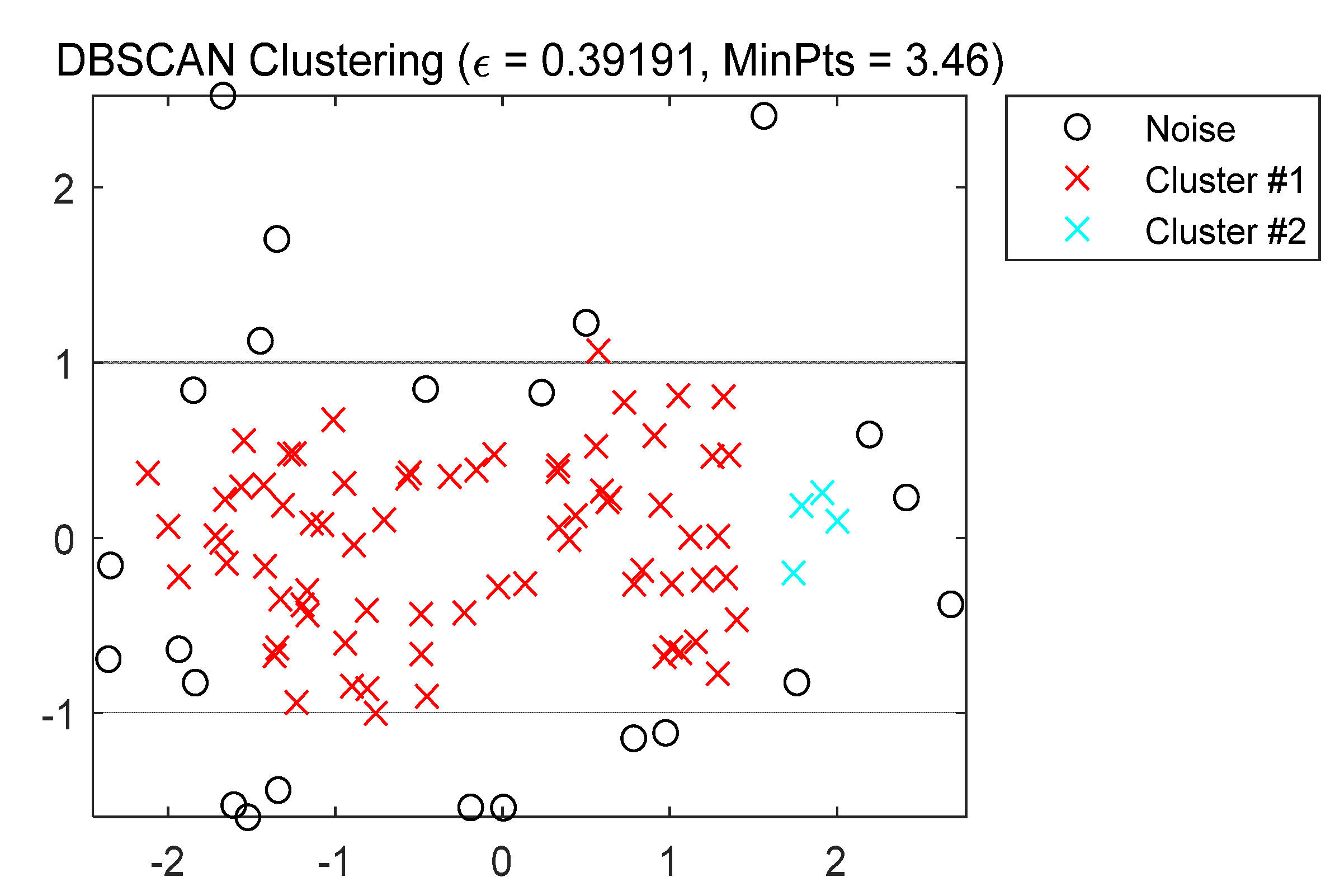
In this paper, ADBSCAN is used to reduce noise to increase the rate of recognition. Because there are too many constellations generated, in order to more intuitively observe the results of noise reduction, the number of symbols sent by simulation is set to 100.
Figure 4 shows that the points in the constellation diagram are divided into two clusters, which are represented by red and blue colors, and the remaining points are labeled as noise points, which will be deleted in the subsequent processing.
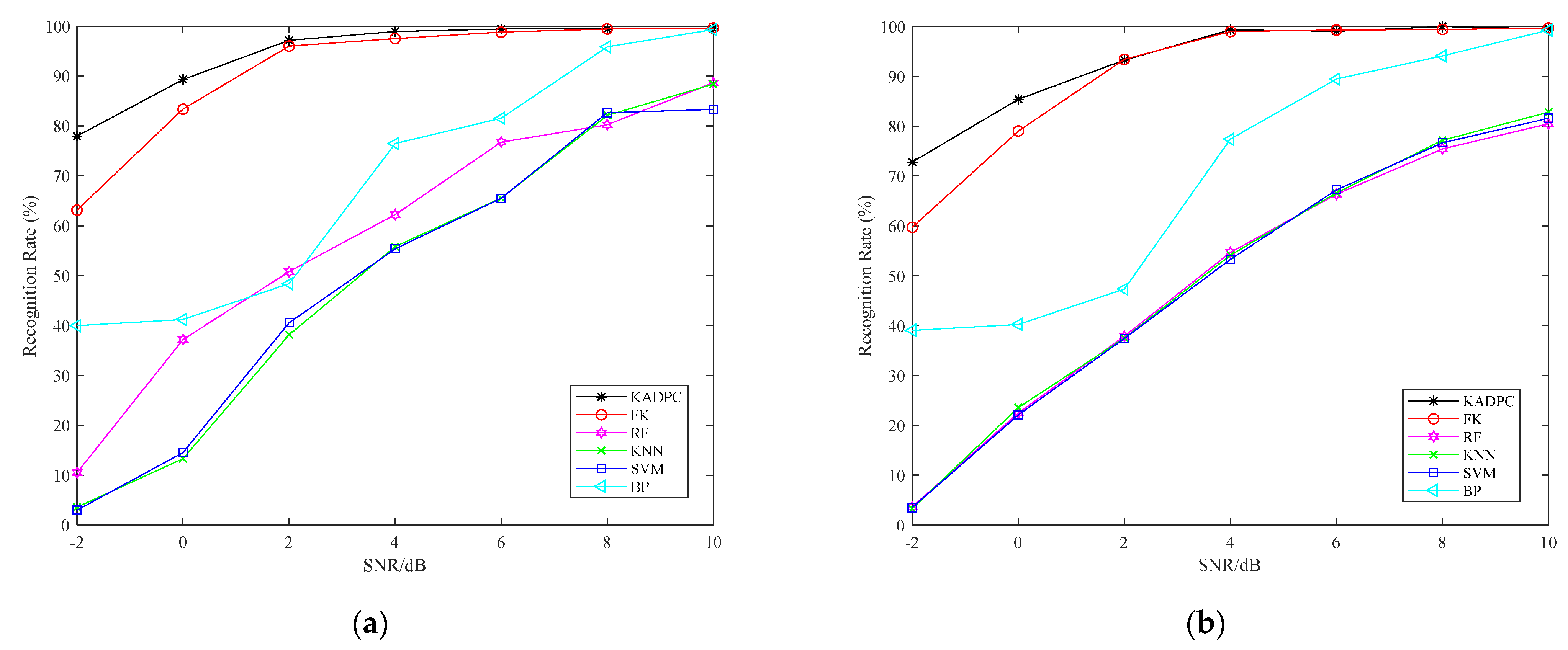
This paper selects several classical algorithms of machine learning and deep learning for comparison, including backward propagation (BP) neural network, fuzzy K-means (FK), random forest (RF), K-nearest neighbor (KNN) and SVM algorithm. Under each SNR, there are 21,000 training samples and 9045 test samples. The recognition rate of BPSK modulated signal under different methods is shown in
Figure 5a. It can be seen that the overall recognition rate curve of KADPC algorithm model is better than other comparison algorithms. The recognition rate curve is stable and close to 100% when SNR = 2 dB. KADPC algorithm adds noise reduction and preprocessing. At the same time, under ideal conditions, BPSK signal has only two clustering centers. When KADPC algorithm is used for feature extraction, the difference of eigenvalues is obvious. Therefore, KADPC algorithm is significantly improved compared with other algorithms.
The simulation results of recognition accuracy of QPSK signal under different SNR are shown in
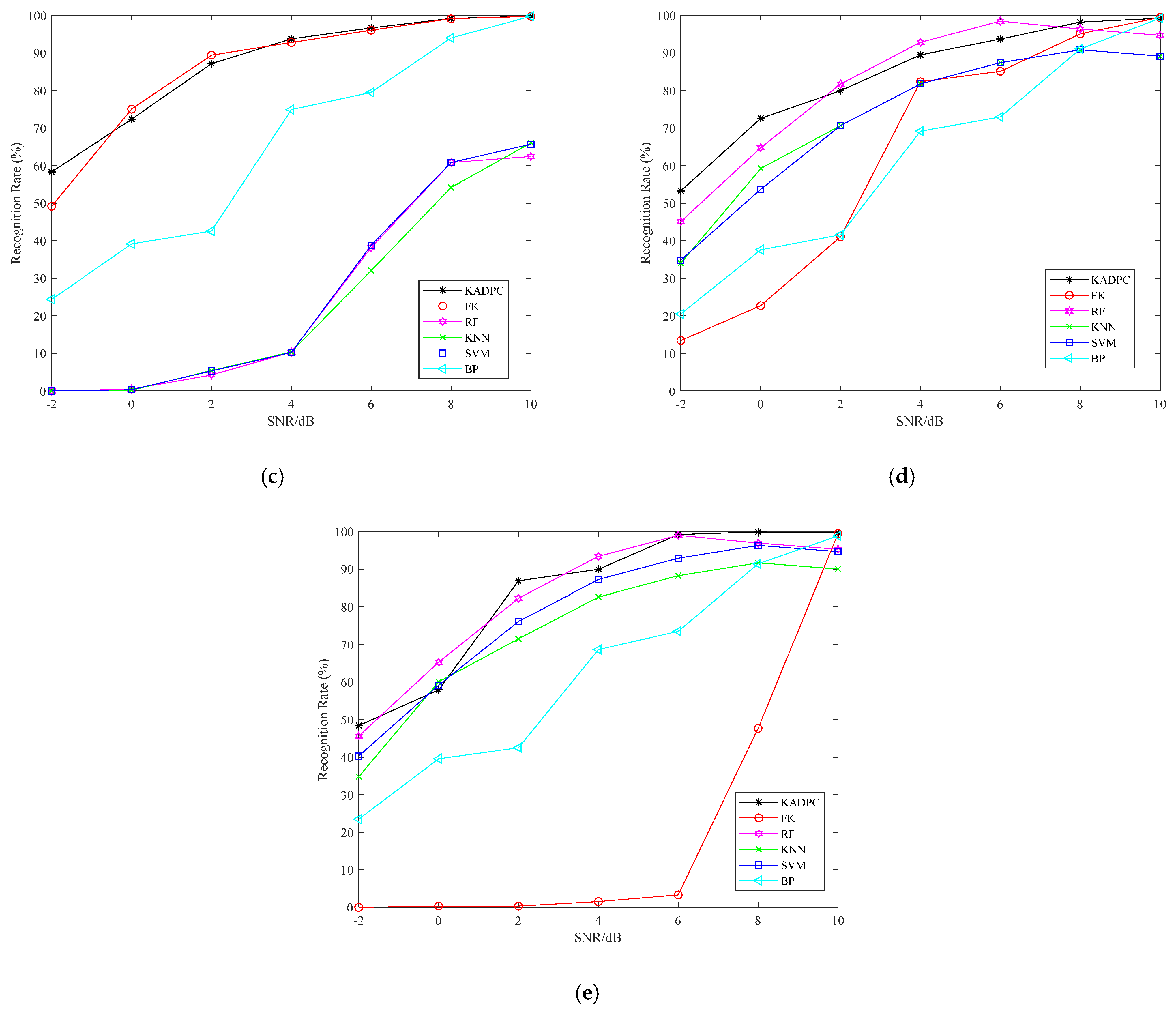
Figure 5b. KADPC model is gradually stable and close to 100% when SNR = 4 dB, while the recognition rate of other algorithms is significantly lower than KADPC algorithm when SNR = 2 dB. Although it is close to that of FK when SNR = 4 dB, it is better than FK algorithm at low SNR. Under ideal conditions, the points in the constellation of QPSK signal are closely distributed around the four clustering centers. With the improvement of SNR, the number of clustering centers of FK is closer to the actual value, so the algorithm is improved significantly. However, the recognition rate of FK is lower than that of KADPC algorithm under low SNR, and the other comparison algorithms perform poorly on QPSK signal. The comprehensive results show that the recognition effect of the algorithm proposed in this chapter is better. The recognition accuracy of 32QAM signal at different SNR is shown in
Figure 5e. It can be seen that the overall curve of KADPC algorithm has higher recognition rate than other algorithms under SNR = 2 dB, and the average recognition rate of the overall algorithm is higher. Because the FK algorithm does not specify the number of clustering centers and uses a fuzzy K value for clustering, the number of clustering centers is farther away from the real value with the increase of modulation order. Therefore, the recognition effect is very poor at low SNR.
The recognition accuracy of the five signals under different SNR is shown in
Table 1. For BPSK signal, it can be seen from
Table 1 that the highest recognition rate of KADPC model is 78.01% at SNR = −2 dB, while the highest recognition rate of other comparison algorithms is only 63.15%. The recognition accuracy of RF, KNN and SVM reach 88.66%, 88.39% and 83.3% at SNR = 10 dB. The results show that the recognition effect of KADPC algorithm proposed in this paper on BPSK signal is better than other comparison algorithms. For 16QAM signal, it can be seen that KADPC model is ahead of the comparison algorithm at SNR = −2 dB, that is to say, KADPC algorithm model combined with noise reduction has better recognition effect at low SNR for 16QAM signal.
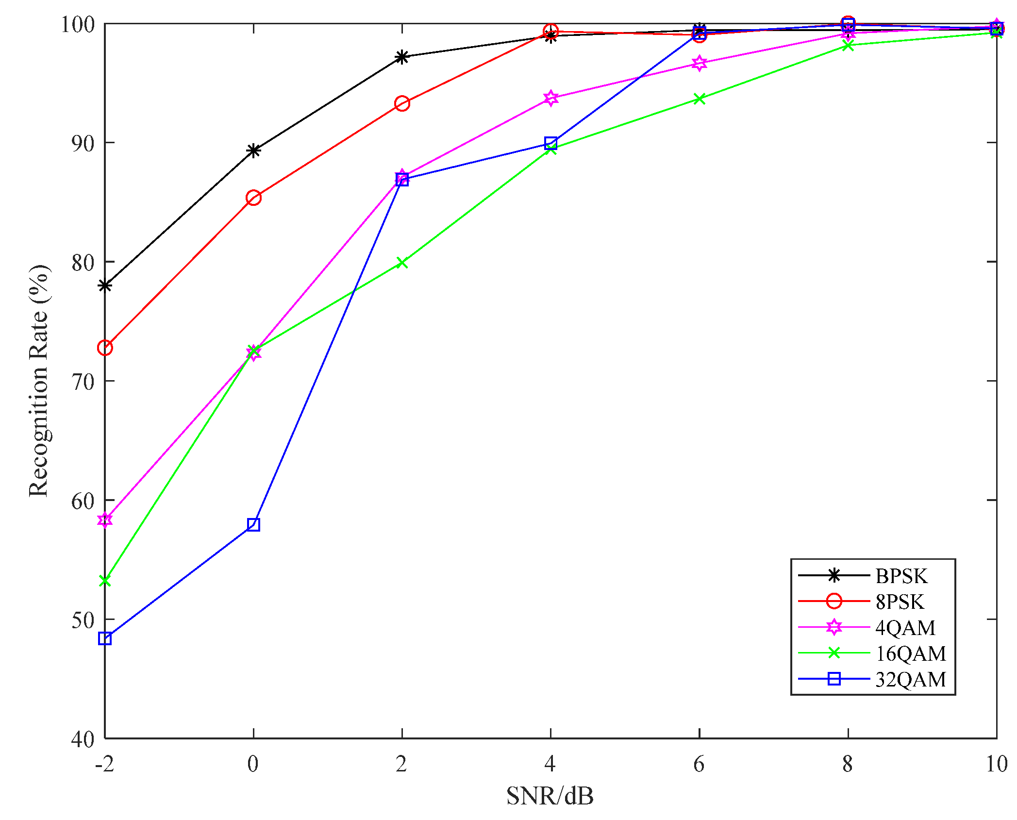
The simulation results show that the recognition accuracy of KADPC model for the modulation modes of five digital signals is shown in
Figure 6. It can be seen that the overall curve of recognition rate increases with the increase of SNR, and the increase of recognition rate decreases with the increase of modulation signal scale. Due to the large noise interference under low SNR, it is difficult for the algorithm to extract the features of the constellation. At the same time, the increase of modulation order leads to the indistinct degree of eigenvalue discrimination. However, generally speaking, the average modulation recognition rate of KADPC algorithm is high and the recognition effect is good.
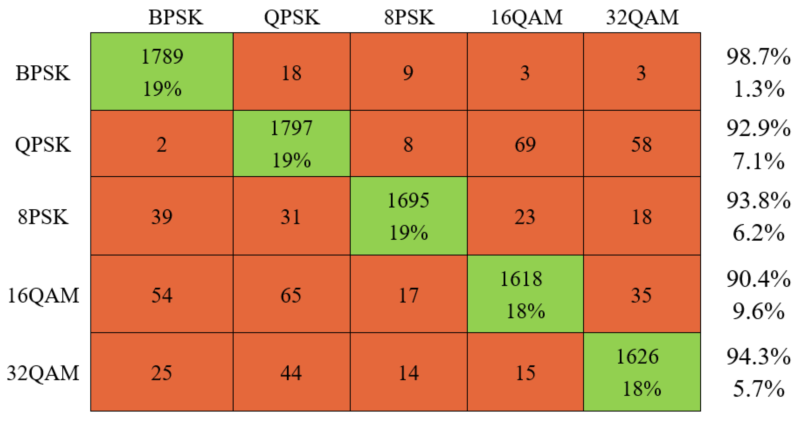
The confusion matrix calculated by KADPC algorithm when SNR = 4 dB is shown in
Figure 7.
The two indexes on the far right are the recognition rate of each signal and the accuracy of the signal from top to bottom. The accuracy is the percentage of the correct modulation mode classification result and the wrong modulation mode classification result in all samples of the modulation mode. The cells on the diagonal represent the correct classification, the percentage is the recall rate. The remaining cells represent the classification error under this SNR. As can be seen from
Figure 7, the KADPC model has great difficulty in feature extraction with the increase of hexadecimal number M. The recall rate of 16QAM and 32QAM modulation types is lower than that of other algorithms. In terms of accuracy and recognition rate, KADPC algorithm has high accuracy and recognition rate when SNR = 4 dB, with an average of more than 90%.
The simulation experimental results show that the recognition rate of the proposed KADPC algorithm in this paper is higher than that of the comparison algorithm under different SNR. Because KADPC algorithm denoises the constellation and uses two clustering algorithms to extract the features of the constellation, which makes the constellation features more concentrated and sufficient, so it presents a better recognition effect as a result. Especially for BPSK, QPSK and 8PSK signals, the effect is ideal, and the applicability is good. Due to the difficulty of feature extraction with the increase of modulation order, the improvement is not obvious for 16QAM and 32QAM signals, but the recognition rate is higher than other comparison algorithms at low SNR. In general, the KADPC algorithm model proposed in this chapter has a good effect on digital signal modulation recognition under different SNR conditions, especially for low SNR.


