Article

Power Quality Monitoring Strategy Based on an Optimized Multi-Domain Feature Selection for the Detection and Classification of Disturbances in Wind Generators

by
David A. Elvira-Ortiz
1,
Juan J. Saucedo-Dorantes
1,
Roque A. Osornio-Rios
1,
Daniel Morinigo-Sotelo
2 and
Jose A. Antonino-Daviu
3,*
1
HSPdigital CA-Mecatronica Engineering Faculty, Autonomous University of Queretaro, San Juan del Rio 76806, Mexico
2
Research Group HSPdigital-ADIRE, Institute of Advanced Production Technologies (ITAP), University of Valladolid, 47011 Valladolid, Spain
3
Instituto Tecnológico de la Energía, Universitat Politècnica de València (UPV), Camino de Vera s/n, 46022 Valencia, Spain
*
Author to whom correspondence should be addressed.
Electronics 2022, 11(2), 287; https://doi.org/10.3390/electronics11020287
Submission received: 24 December 2021 / Revised: 12 January 2022 / Accepted: 13 January 2022 / Published: 17 January 2022
(This article belongs to the Special Issue Robust Design Optimization of Electrical Machines and Devices)

Abstract

:
Wind generation has recently become an essential renewable power supply option. Wind generators are integrated with electrical machines that require correct functionality. However, the increasing use of non-linear loads introduces undesired disturbances that may compromise the integrity of the electrical machines inside the wind generator. Therefore, this work proposes a five-step methodology for power quality disturbance detection in grids with injection of wind farm energy. First, a database with synthetic signals is generated, to be used in the training process. Then, a multi-domain feature estimation is carried out. To reduce the problematic dimensionality, the features that provide redundant information are eliminated through an optimized feature selection performed by means of a genetic algorithm and the principal component analysis. Additionally, each one of the characteristic feature matrices of every considered condition are modeled through a specific self-organizing map neuron grid so they can be shown in a 2-D representation. Since the SOM model provides a pattern of the behavior of every disturbance, they are used as inputs of the classifier, based in a softmax layer neural network that performs the power quality disturbance detection of six different conditions: healthy or normal, sag or swell voltages, transients, voltage fluctuations and harmonic distortion. Thus, the proposed method is validated using a set of synthetic signals and is then tested using two different sets of real signals from an IEEE workgroup and from a wind park located in Spain.

1. Introduction

Modern society is experiencing a series of challenges in matters of power generation associated with the use of fossil fuels in the power generation process. This situation has led to an increase in greenhouse gas emissions, which has caused severe air pollution problems [1]. Moreover, fossil fuels are non-renewable resources that have become increasingly depleted in recent years, resulting in a rise in their prices [2,3]. To deal with these problems, power generation has started using use renewable sources as fuels (such as sunlight and wind); in fact, nearly one-third of the global electricity demand is fulfilled only with the use of renewable energies [4]. Among all the renewable energies, wind energy among the most widely spread, because it is mature from a technological point of view, it presents a competitive levelized cost of energy (LCOE) and it is relatively easy to obtain an important amount of energy by means of this renewable resource [5]. Nonetheless, the use of wind energy implies some important challenges. For instance, the amount of generated energy is location-specific, and a study of the wind conditions in the location is required to properly select the wind turbine and to guarantee that energy production is sufficient to represent monetary earns [6]. Also, the policies regarding wind generation are different from one country to another [7]. Additionally, wind generators are complex systems that combine mechanical, electric, and electronic devices to transform wind energy into electricity, and they must provide a robust, reliable, and high-quality power supply. Maintaining this high-quality supply is a challenge due to the large amount of non-linear loads that are used nowadays. These non-linear loads introduce a high number of harmonics that contaminate the power grid and cause waveform distortion. An electric grid that presents power quality (PQ) issues generates damages in domestic loads and leads to unexpected stops at industrial facilities that will translate into financial losses. In this sense, the electric generator becomes of great importance in any wind turbine. Therefore, in order to optimally design a wind generator, it is necessary to develop strategies that allow determining the existence of failures that compromise the quality of the generated energy. PQ problems cause erratic operation of electronic controllers and computer data loss [8]. They also lead to the inappropriate operation of relays, programmable logic controllers, and computers. Therefore, the methodologies for disturbance detection allow for improving the design of wind generators and preventing the malfunctioning of their components.
PQ monitoring has been widely explored, and several techniques have been developed to determine the presence of waveform distortion or power quality disturbances (PQD) in electrical signals. To properly perform this identification, it is important to carry out a feature extraction that provides information regarding the occurrence of any event. One of the most common techniques for this feature extraction is the Fourier transform (FT) [9,10], which delivers good results in the evaluation of stationary disturbances such as harmonic distortion. However, the conventional FT-based methodologies present some important drawbacks, such as the existence of spectral leakage and the fact that this technique cannot be applied in the analysis of transient disturbances. Moreover, the FT cannot provide temporal information related to the occurrence of the PQD. To overcome the issues related with the FT, some other time-frequency transforms have been explored, for instance, the short-time Fourier transform [11], S-transform [12]; the wavelet transform [13]; empirical mode decomposition (EMD) [14]; and the Hilbert Huang transform [15], among others. These techniques are able to detect not only stationary PQD but also non-stationary PQD; furthermore, they provide accurate information associated with the time when the disturbance occurs. However, these time-frequency techniques demand a higher computational effort and lose accuracy in frequency information, since they work with modes that contain a group of frequencies instead of a single frequency component. Also, they suffer from mode mixing, so the information regarding a specific PQD can appear in more than one mode, hindering the disturbance identification. This is why some other works prefer to extract features like high-order statistics (HOS) directly in the time domain [16]. The use of HOS features presents some interesting advantages; for instance, the insensitivity to Gaussian noise and the low computational burden. On the other hand, HOS are highly sensitive to window size, and the use of a different number of samples of the same signal may lead to different results, especially when the PQD is short. Finally, it is important to mention that all the aforementioned techniques can be implemented to work along with artificial intelligence techniques such as artificial neural networks (ANN) [17], fuzzy logic-based classifiers [8], support vector machines [18], genetic algorithms (GA) [19], and even with some deep learning approaches [20]. This combination of strategies allows for performing an automatic classification of the founded PQD accurately. Yet, the number of extracted features in all the aforementioned approaches can be high, and many of them do not deliver important information regarding the existence of a specific disturbance. Thus, it is necessary to develop strategies to perform a proper feature selection. Specifically speaking of power quality in grids with injection of wind energy, it has been reported that the disturbances that more commonly appear are harmonic distortions, notch, voltage swell/sag, momentary interruptions, and voltage fluctuations [21]. To deal with these issues, some wind generators incorporate distribution static compensators [22] or passive and active filters [23,24]. These devices are intended to suppress the presence of harmonics and to work as reactive power compensators, and the PQ of the grid improves as a result of their action. Since, in this field, attention is focused on the development of devices for mitigating PQ issues, there is a lack of methodologies for the detection and identification of disturbances. Nonetheless, the development of techniques for PQ analysis can work along with the devices for PQ issues mitigation, because they can estimate the features required for tuning the filters and compensators used in wind turbines. Additionally, information from PQ monitoring allows for improvement in the design of blades, mechanical transmission systems, electric generators, in order to obtain a more reliable and robust machine.
Indeed, several methodologies have been reported for carrying out optimal feature selection in order to discard redundant information. Thus, some optimization techniques, like k-means [25] and bio-inspired algorithms [26], are used to set a model that describes the behavior of the PQD and select the features that better describe such behavior. In this way, it is possible to reduce the required computational effort and to increase the efficiency of the results. Also, in recent years, the use of dimensionality reduction techniques such as the linear discriminant analysis (LDA) [27] and principal component analysis (PCA) has been explored [28] for dealing with a complex set of features and reducing it to a three-dimensional or two-dimensional view. Additionally, with the use of these techniques, it is possible to maximize the distance between clusters, making the classification process more efficient and accurate. The aforementioned works use features in only one domain (time, frequency, or time-frequency); therefore, they are prone to experience difficulties when dealing with disturbances that exhibit similar behaviors in the analyzed domain. Hence, in [29], a multi-domain feature extraction for discerning between PQD with similar behavior is proposed; then, using an autoencoder, a dimensionality reduction is performed to facilitate the classification process. The problem with the multi-domain feature extraction is that the number of features to be considered highly increases. In this sense, using an optimization technique for feature selection may be helpful for reducing the effort required in the dimensionality reduction process. In terms of wind turbines, these methodologies have been used for the detection of failures in the components of the mechanism. For instance, in [30], PCA is used along with Hoteling’s T2 method to assess the condition of the electric generator in a wind turbine. On the other hand, in [31], different variables such as active power, wind speed, rotor velocity, and blade angle are measured in a wind power installation. A generalized regression neural network ensemble for single imputation is used for feature extraction in all the measured variables and then, a feature reduction is performed using PCA. Finally, the wavelet-based probability density function is implemented, with the aim of identifying blade failures. Although these works deal with the identification of undesired conditions in wind turbines, they only consider the condition of the machine, and the PQ is left aside. It is important to pay more attention in the detection of PQD, since considering them is helpful for the general design of the wind generation system.
Thereby, the main contribution of this work relies in the proposal of a strategy for optimal feature selection that allows for modeling electric signals through statistical features in different domains that are used to better characterize the behavior of a PQD. The proposed methodology considers as a first step the implementation of a multi-domain feature extraction. Since the resultant number of features is high, a GA–PCA optimization is carried out to eliminate those features that provide redundant information. Then, a feature learning stage is implemented. In this step, self-organizing maps (SOM) are used to obtain a model of the PQD in the time, frequency and time-frequency domains. Finally, the SOM models obtained in every domain are used as inputs of a softmax layer ANN that works as the classifier. In the present work, both stationary and non-stationary disturbances are considered. Among the wide variety of PQD, only the following are considered: harmonics and voltage fluctuations for the stationary disturbances; and voltage sag, voltage swell, and transients (impulsive and oscillatory) for the non-stationary disturbances. These disturbances are selected because their appearance is common in grids that include renewable resources such as wind generation. The training and validation of the proposed strategy are performed using a set of synthetic signals that are modeled to be a reliable representation of electrical signals containing PQD. Then, the methodology is tested using two different groups of real signals. The first set is provided by the IEEE 1159.3 working group, whereas the second one corresponds to a series of measurements taken in a real wind farm located in northern Spain. As previously mentioned, the existence of PQD can produce a malfunction of the components of the machine; therefore, this methodology aims to be a tool for detecting PQD and improving the reliability of the wind turbine by preventing its failure. In this way, the designers and manufacturers of wind turbines can consider the existence of PQD during the entire production process in order to improve the quality, not only of the power supply, but of the entire generation system.

2. Theoretical Background

2.1. Self-Organizing Maps

The self-organizing map (SOM) is a novel unsupervised machine learning technique, whose main purpose consists of performing a non-liner projection of a high-dimensional input data set into a low-dimensional space. SOM is based in a neural network that requires a pre-defined number of neurons to resemble and map the data distribution of the input space. The use of SOM presents an interesting advantage against other methodologies for PQ monitoring, and due to its capability for automatically adjusting to different data topologies, the SOM may be used as a learning algorithm for mapping an input feature space and model that can be considered the normal behavior, and then identifying patterns that differ from this normality and classifying them according to the topological characteristics of the data input [32].
An SOM model is composed of two main layers of neurons as it is presented in Figure 1; the input layer is composed of N neurons, where each one represents an input variable of the input feature space; through the input layer, the received information is transmitted to the output layer. The output layer comprises predefined M neurons and, in this layer, aims to automatically adapt the input feature space in order to obtain a characteristic pattern map. Each neuron of the grid in the output layer represents a matching unit (MU). Normally, the neurons in the output layer are arranged in the form of a two-dimensional map, which is also known as the resulting SOM neuron grid. As Figure 1 shows, the connections between the two layers of the SOM network are always forward; that is, the information of the input feature space is propagated from the input layer to the output layer. Thus, each input neuron i is connected to each of the output neurons j by a weight ω j i ; in this way, the output neurons are associated with a vector of weights W j that is called the reference vector or codebook, since it constitutes the prototype or average vector of the category represented by the output neuron j. Thus, the SOM model defines a projection from a high-dimensional data space into a two-dimensional neuron grid map of neurons [32,33,34].
The SOM learning process can be described by two main steps as follows: step (i) A vector x is randomly selected from the input feature space and its distance or similarity to the vectors m j , in the codebook, is calculated, using, for example, the Euclidean distance (1):
x m j = min j { x m j }
Once the closest vector or BMU (best matching unit) has been found, the rest of the vectors in the codebook are updated. Step (ii) the BMU and its neighbors, in the topological sense, move close to the vector x in the input feature space. The magnitude of this attraction is described by the learning rate, which is also known as the topological error ( E ¯ t ). As the learning process proceeds and new vectors are assigned to the neuron grip map, the learning rate gradually decreases towards zero; consequently, the neighborhood radius also decreases. The update or learning rule for the given reference vector i is defined by (2):
m j ( t + 1 ) = { m j ( t ) + α ( t ) [ x ( t ) m j ( t ) ] m j ( t )   j N c ( t ) j N c ( t )
where, t is the discrete-time index for the variables, α ( t ) [ 0 , 1 ] is a scalar that defines the relative size of the learning step, and N c ( t ) specifies the neighborhood around the winner in the map array.
Then, steps i and ii are repeated until the training process ends. The number of training steps must be pre-defined a priori to calculate the convergence rate of the neighborhood function and the learning rate. Once the training is finished, the resulting neuron grip map is ordered in a topological sense: n topologically close vectors are applied in n adjacent neurons or even in the same neuron. Moreover, to determine whether the resulting SOM neuron grid has been properly adapted to the input feature space during the training process, as measures of quality of the maps, the precision of the projection and the preservation of the topology are considered. The projection precision measure describes how neurons adapt or respond to input feature space. Usually, the number of data points is greater than the number of neurons, and the precision error is always different from 0. To calculate the precision of the projection, the mean quantization error ( E ¯ q ) over the complete input feature space is estimated as (3):
E ¯ q = 1 N i = 1 N x i m c
Also, as aforementioned, the topology preservation measure describes how the SOM neuron grid preserves the topology of the input feature space. This measurement considers the structure of the neuron grid map, i.e., on an oddly twisted map, and the topographic error is large even if the precision error is small. Thus, the topological error, E ¯ t , can be calculated by following (4):
E ¯ t = 1 N i = 1 N u ( x k )
where, u ( x k ) is equal to 1 if the first and second BMUs of x k are not close to each other, otherwise, u ( x k ) is equal to 0.
An additional advantage of using SOM to model an input feature space is that SOM performance is qualitatively measured in terms of the E ¯ q , that also provides information regarding the detection of unknown events that do not match with the topology of input feature space used to create a SOM neuron grid model. In Figure 2a–c, general and visual descriptions that depict the learning procedure performed to model a SOM neuron grid are shown.

2.2. Power Quality Definitions

The term power quality is used for defining a wide variety of electromagnetic phenomena that occur at a certain time and location on the power system. These phenomena result in the parameters that describe an electrical signal, like frequency and amplitude, deviating from the ideal values, causing waveform distortions. According to the IEEE standard 1159–2019 [35], voltage sag and voltage swell are RMS variations. The former occurs when RMS voltage decreases to a value between 0.1 pu and 0.9 pu; the latter is represented by an increment of the RMS voltage to values above 1.1 pu. The same standard defines a transient event as a disturbance that is undesirable but momentary in nature. These events are classified into two categories: impulsive and oscillatory. A sudden nonpower frequency change from the nominal condition that is unidirectional in polarity is known as impulsive transient; in contrast, when an electrical signal presents a sudden nonpower frequency change in the steady-state condition that includes both positive and negative polarity values, then it is said that an oscillatory transient has occurred. Additionally, voltage fluctuations are defined as systematic variations of the signal envelope causing the peak value of the voltage signal to oscillate between 0.95 pu and the 1.05 pu. Finally, harmonics are sinusoidal components that are integer multiples of the fundamental frequency (usually 50 Hz or 60 Hz). When harmonics are combined with the fundamental component, they produce a waveform distortion that is evaluated using a quantity called the total harmonic distortion (THD). The IEEE standard 519–2014 [36] establishes that the THD level must remain under the 8% in grids that handle voltages lower than 1.0 kV. All the aforementioned disturbances can be mathematically modeled, and Table 1 shows the equations that describe them.
The parameters in Table 1 are described in detail as follow: A is the amplitude of the fundamental component; f f c is the frecuency of the fundamental component; k is the discrete number of sample; ϕ is the phase angle in radians; α represents an amplitude deviation; k 1 is the sample where the disturbance begins; k 2 is the sample where the disturbance ends; ψ corresponds to the amplitude of the transients, f f l is the frequency of the voltage fluctuations; M is te total number of harmonics; and A h is the amplitude of every single harmonic.

3. Methodology

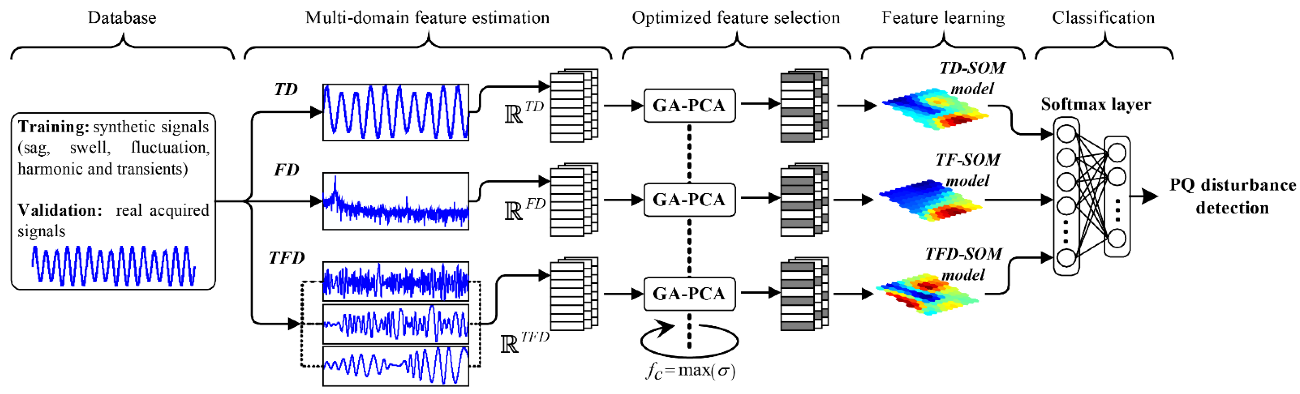
As mentioned, in the design of electric machines such as wind generators, it is important to consider the identification of failures and situations that compromise the quality of the power supply and, therefore, the integrity of the loads attached to the grid. In this regard, Figure 3 presents the flowchart of the proposed strategy that focuses on the identification and classification of PQD through an optimal multi-domain feature selection. The methodology has been designed to follow a step-by-step scheme to make its comprehension and application easier. A total of five stages compounds the PQ monitoring strategy: database, multi-domain feature estimation, optimized feature selection, feature learning and classification, where this final stage delivers the PQ disturbance detection as output. Every step is described in detail in the following subsections.

3.1. Database

This work considers the use of synthetic and real signals. The former are used in the training process whereas the latter are used for validating the results of the proposed strategy.
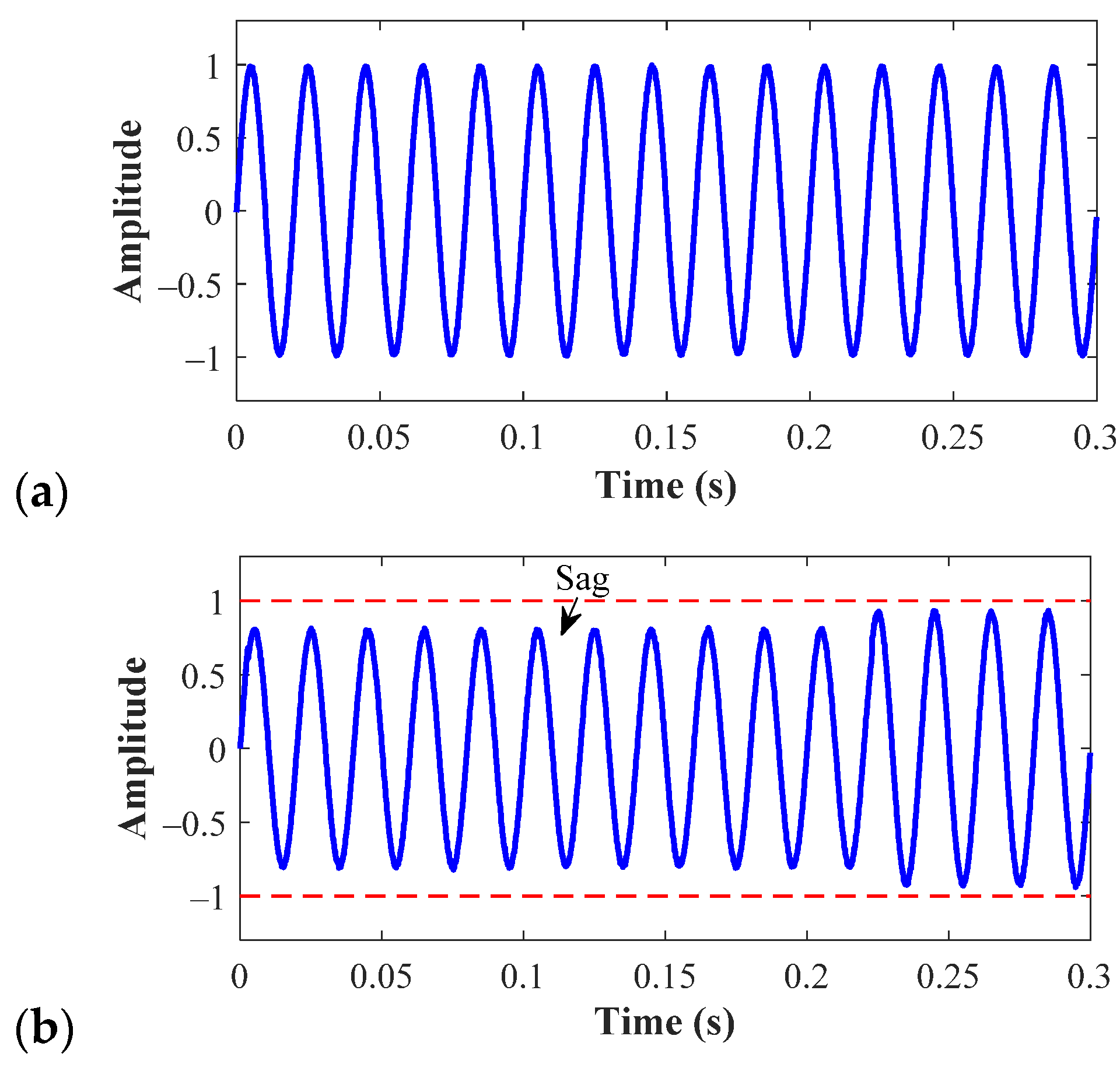
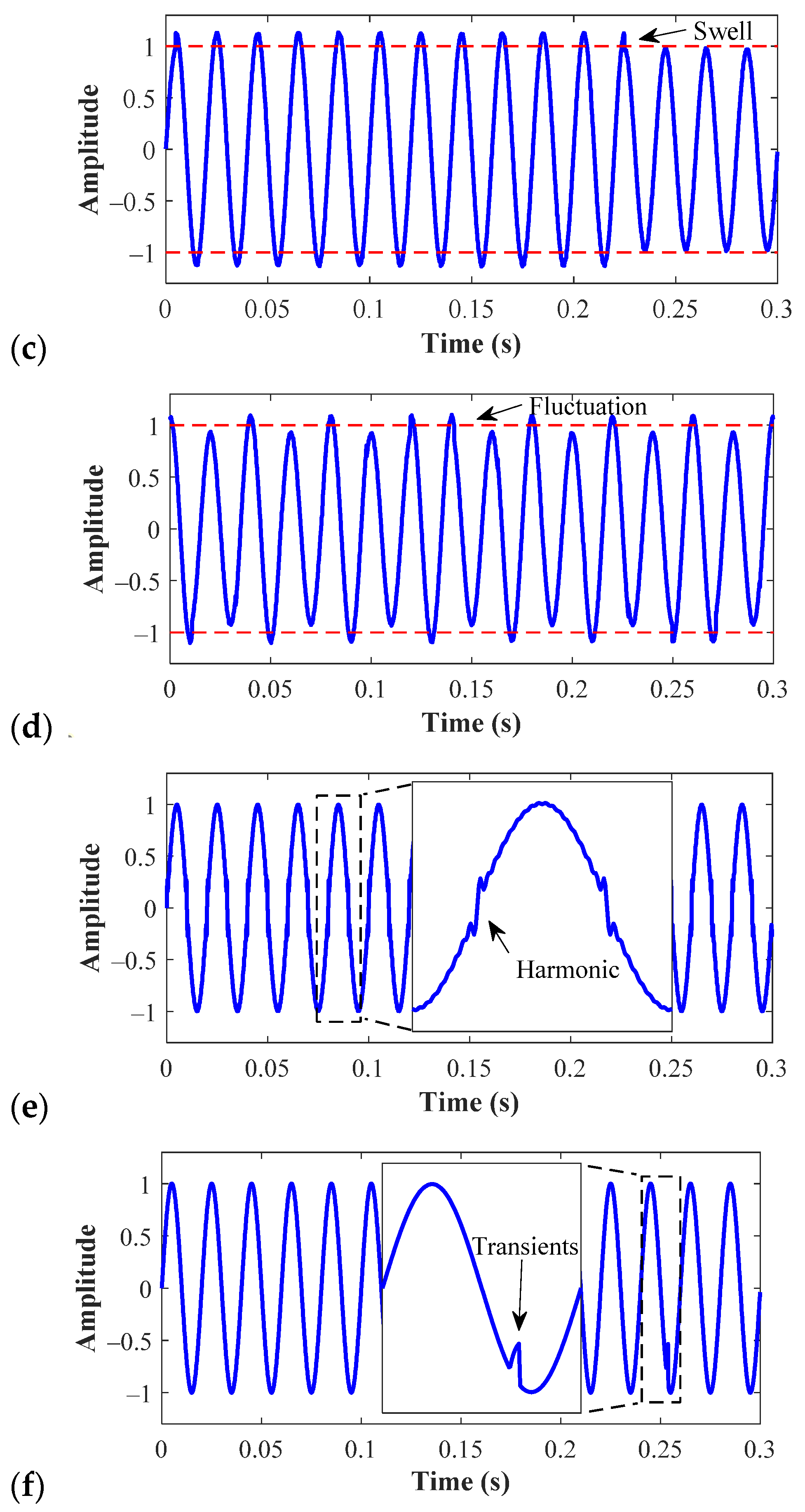
The synthetic signals are generated with the purpose of representing six different conditions of electrical signals: a healthy signal (i.e., a signal without any disturbance), a voltage sag, a voltage swell, transients (impulsive and oscillatory), voltage fluctuations, and harmonic distortion. Considering the definitions stated by the IEEE standard 1159–2019, the mathematical models presented in Table 1 are used for generating the set of synthetic signals.
Before continuing, it is important to address some facts. For instance, all the parameters presented in the third column of Table 1 are randomly generated considering the range of values established in the same table. Also, the term f f c , which represents the frequency of the fundamental component, is considered as 50 Hz. Moreover, for the case of harmonics, the number of harmonics and the amplitude of harmonicas is randomly selected, but in all the cases, a THD value higher than 8% must be accomplished to consider those cases with unacceptable harmonic distortion. Additionally, the model presented for the description of transients corresponds to an impulsive transient. Although impulsive and oscillatory transients are different and they can be described with different parameters, for the sake of simplicity, in this work, it is considered that an oscillatory transient can be expressed as an impulsive transient that appears more than one time with different values; therefore, the classifier will detect both disturbances only as transients. Also, it is considered that all the signals are generated using a sampling frequency of 8 kHz and with a duration of 300 ms. Finally, 100 signals per condition are generated to obtain a total of 600 elements that will be used in the following stages of the training process.
Regarding the real signals, these are taken from two different data sets. A first data set is provided by the IEEE 1159.3 working group [37], and it consists of a series of voltage and current signals, recorded from different real locations, with diverse PQD. The data set is formed by over 300 signals, but to validate the correct performance of the proposed strategy, only 3 cases are presented: transients, a voltage sag, and a voltage swell. In these signals, it is considered that the fundamental frequency is 60 Hz, and the signals are acquired at different sampling rates. For instance, the signal with the transients is acquired at a sampling rate of 15,360 Hz, whereas the signals with voltage sag and voltage swell are acquired considering a sampling frequency of 7680 Hz. The second set of real signals is acquired from a 30-MW wind park located in northern Spain. A proprietary data acquisition system (DAS) is used for collecting and storing electrical signals. This DAS is based on field-programmable gate array (FPGA) technology and it is able to acquire data from 7 channels simultaneously. The sampling rate of these signals is 8 kHz and the fundamental frequency is 50 Hz. At this location, a total of 4 different cases are presented: one for a healthy signal, another one for voltage sag, one more for transients, and, finally, one for harmonic distortion. Both sets of real signals are used to assess the performance of the proposed strategy under real conditions. However, the proposed methodology aims to be a tool for wind turbine designers; therefore, the results obtained with the second set of real signals come to be of great importance for validating the reliability of this strategy.

3.2. Multi-Domain Feature Estimation

It has been previously addressed that for PQD that present similar behaviors, a multi-domain approach may be helpful for obtaining better classification. Thus, h the use of three different domains is proposed here: time domain (TD), frequency domain (FD), and time-frequency domain (TFD). However, before performing any feature estimation, it is necessary to perform an amplitude normalization of the electrical signal; such normalization is carried out considering the nominal RMS value of the voltage signal. Therefore, all the amplitude values are dimensionless and expressed as per unit (pu). This consideration is implemented because the data sets that are used in this work consider signals from different grids and, therefore, have different nominal amplitudes. Nevertheless, by performing this normalization, the proposed methodology is able to properly work, even for signals with different nominal amplitude values.
In the case of the TD feature estimation, the 15 statistical features summarized in Table 2 are calculated for every signal. Therefore, the dimensionality of this space is set as TD = 15 and a feature matrix composed by statistical time domain features is obtained, T D     TD . In the case of the FD analysis, first, it is necessary to compute the fast Fourier transform (FFT) of each normalized signal to obtain its representative spectrum. Then, the 14 statistical features presented in Table 3 are estimated over the signal spectrum. Hence, the dimensionality of this new space is FD = 14 and a representative FD-dimensional feature matrix, F D     FD , is obtained. At this point, it is important to address the fact that the statistical features are estimated over the amplitude values of the signal spectrum. Since the signals have been previously normalized, it is expected that the fundamental component presents an amplitude of 1 pu in a healthy condition, and any variation from this value will be related with the existence of a disturbance. Moreover, since only the amplitude values of the spectrum are considered, the proposed methodology can be applied in any signal, regardless the value of the fundamental frequency. This turns to be one of the main advantages of the proposed approach, because it can be applied in 60 Hz grids and also in 50 Hz grids without requiring any modification. Finally, to carry out the TFD feature estimation, a preprocessing of the normalized signals is required prior to feature estimation. This preprocessing task consists of performing a signal decomposition, and the EMD technique is used for this purpose. The result of applying the EMD over the voltage signals is a set of sub-signals that show the main oscillatory modes of the original signal and that are called intrinsic mode functions (IMF). An important drawback of the EMD technique lies in the fact that it is not possible to have a priori knowledge of the IMF that can be obtained from a particular signal. Moreover, when the EMD is applied over two different signals, it is possible that a different number of IMF is obtained from each signal. To consider that a signal provides significant information in the TFD, only those signals that deliver 3 or more IMFs after applying the EMD are considered; the rest are discarded. Once the preprocessing task has been applied, the set of 15 statistical features presented in Table 2 are individually estimated over the three first resulting IMFs. So, for this last space, the dimensionality turns out to be TFD = 45 , and, as in the previous cases, it is possible to obtain a TFD-dimensional feature matrix, T F D     TFD . As in the previous cases, the feature estimation is performed over the amplitude values of every IMF; therefore, the methodology is insensitive to variations in the value of the fundamental frequency, and it can be applied in both 60 Hz and 50 Hz grids.
At this point, it is important to mention that, in the case of the training process, every synthetic signal is generated with a duration of 300 ms, and the feature estimation is performed over the complete signal. In the case of the real signals, they present different durations: if the length of the real signal is less or equal to 300 ms, the feature extraction is carried out over the complete signal; if the length of the signal is more than 300 ms, the signal is divided in windows of 300 ms and the statistical features are extracted for every window. Moreover, this proposed approach is intended to be applied offline, even with the real signals.

3.3. Optimized Feature Selection

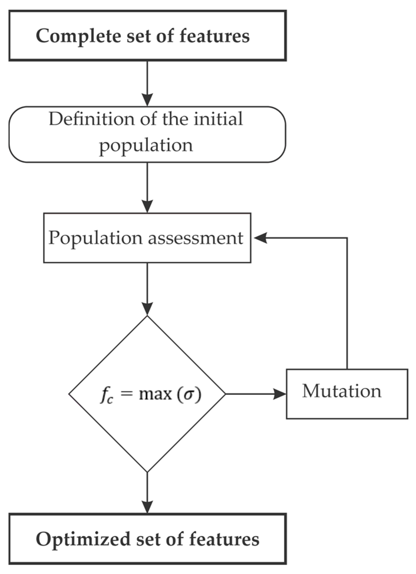
Considering the three proposed domains (TD, FD and TFD), a total of 74 statistical features are estimated. This is a considerable number of features, and there is no guarantee that all of them provide valuable information regarding the PQD behavior. This is why it is necessary to perform an optimization in the feature selection process. For this purpose, the fusion of two different techniques, GA and PCA, is proposed. GA is a heuristic search algorithm based in Darwin’s natural selection. This technique has been widely used for solving optimization problems because of its ability for minimizing estimation errors. GA requires an objective function that will be the one in charge of defining the goodness of fit (GOF) in the optimization task. In this work, the objective function for the GA is directly stated by the PCA, a mathematical procedure that allows performing a reduction in the dimensionality of a problem, preserving the variability of the data. To assess the variability that has been preserved by the PCA, the data variance is used, and it is precisely this value of the parameter that will be used for the GA to perform the optimization task. The complete optimized feature selection is carried out following the procedure proposed in [38] and illustrated in Figure 4 as described below:
Stage 1: Definition of the initial population. It is considered that the population that will be held by the GA is composed of a logical vector that counts with a total of 74 chromosomes, where every chromosome represents each one of the statistical features previously estimated. A chromosome takes a value of zero if the statistical feature that represents is not considered in the evaluation process, and it takes a value of one if the statistical feature is being considered in the analysis. Thus, the initial population is randomly generated by considering that at least one of the elements contained in the logical vector has to be selected to be evaluated; also, more than one element can be evaluated. Once this task has been fulfilled, the procedure goes to stage 2.
Stage 2: Population assessment. At this point, the fitness function of the GA must be selected to assess the performance of each individual. In this particular case, the fitness function is defined in terms of the accumulation of the data variance. This cumulative variance is calculated using the PCA, and the fitness function comprises the cumulative variance of the two and three first principal components. In this sense, the optimization problem that must be solved by the GA consists of searching for the specific statistical features that maximize the cumulative data variance delivered by the PCA. Once the whole population is evaluated, the condition of best features obtained is analyzed; therefore, the next stage is 4.
Stage 3: Generation of a new population. The GA has two operations that allow to generate a new population preserving the values that positively contribute to reach the optimization goal. These operations are the crossover and the mutation. Here, the common single-point crossover operator and the roulette wheel selection are in charge of generating this new population. In this way, it is possible to take the chromosomes of the previous population that present the highest fitting values (higher data variance), and keep them for the new population. Also, to prevent stagnation and to provide the new population with fitness variability, the mutation operation is applied using a Gaussian distribution. Next, the new population has to be evaluated; thus, the algorithm continues in stage 2.
Stage 4: Stop criteria. There are two different constrains that determine if the GA must finish its execution. The first one occurs when the optimization problem is solved and the GA finds the features that reach the highest maximization of the data variance; the second one consists on reaching a maximum number of generations (iterations). When one of the stop criteria is reached, the GA delivers the optimized set of features and the iterative process finishes; otherwise, the process is iteratively repeated until one of the stop criteria is reached. If the stop criteria are not met, then the algorithm continues in stage 3.
The described procedure is applied to each domain separately; therefore, three optimized feature sets are obtained: one for the TD, other for the FD and a third one for the TFD. Then, the feature learning step only receives the sets of features that reached the maximum cumulative variance. Therefore, as a result of the optimized feature selection, the dimensionality of each one of the domains has been reduced. This situation is helpful for the next steps in order to obtain a better characterization of each disturbance.

3.4. Feature Learning

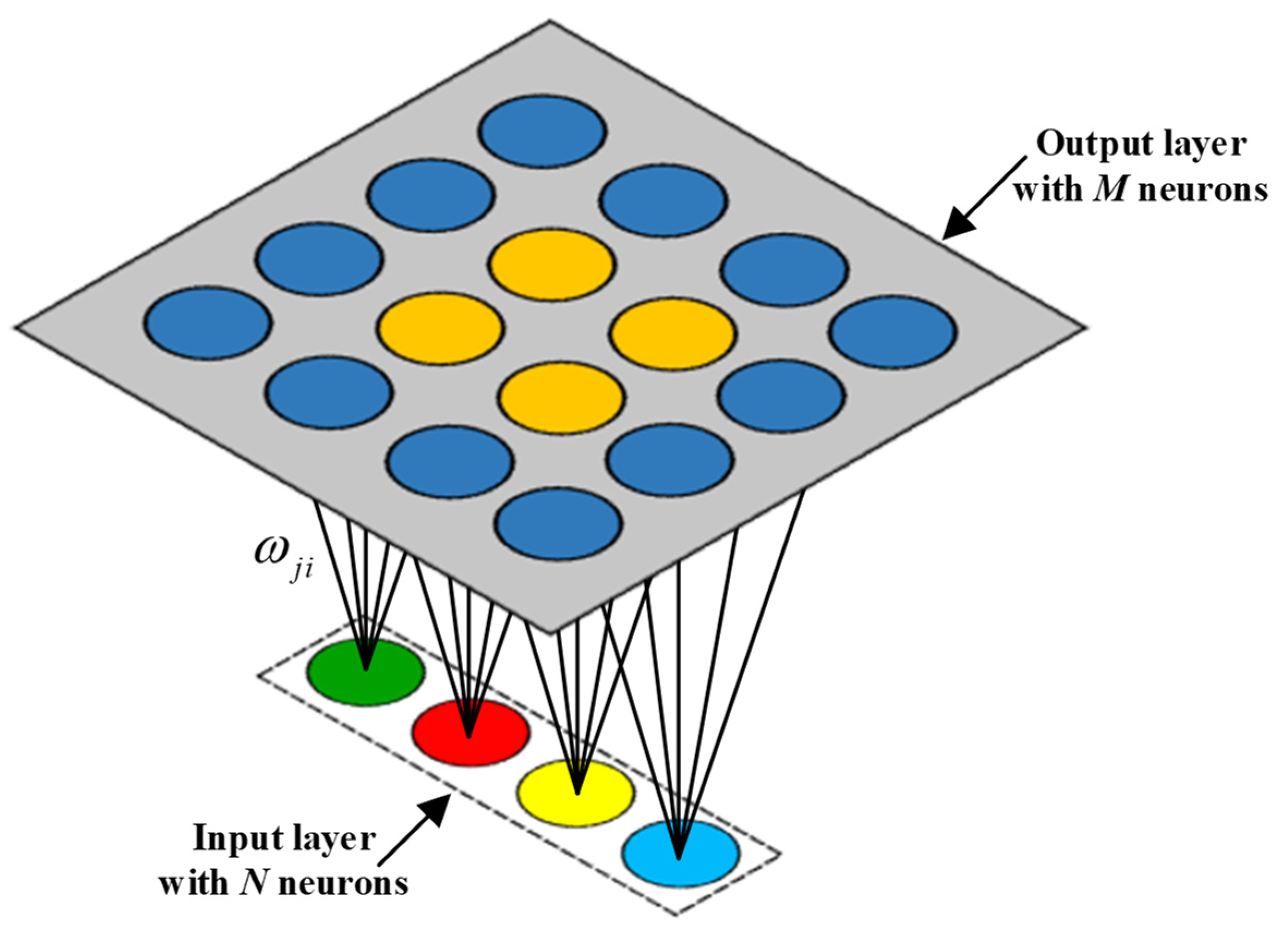
The feature learning stage is performed by means of using the SOM unsupervised algorithm, and the objective of this stage lies in modeling those selected sets of features that better characterize each of the evaluated conditions for the three domains of analysis, TD, FD and TFD. In this regard, different SOM neuron grids are generated, as many feature matrices are available, where there exist three available feature matrices that characterize each one of the evaluated conditions. Therefore, several SOM neuron grids are generated with a pre-defined number of neurons, i.e., defined with 100 neurons over a 10 × 10 grid, and then each one of the available feature matrices is subjected to the feature learning. Thereby, the resulting SOM neuron grids may represent each one of the different evaluated conditions (healthy or normal, sag or swell voltages, transients like impulsive and oscillatory, voltage fluctuations and harmonic distortion) and the original d-dimensional space of the input feature spaces are then represented into a 2-dimensional neuron grid. Once the feature learning is carried out, for each SOM neuron grid model, the pre-defined neurons known as matching unit (MU) are adapted to the input feature spaces or characteristic feature matrices preserving the topological properties that represent a high-performance feature characterization of the assessed conditions.

3.5. Classification

The idea of performing an optimized feature selection and then the modeling of the disturbances under evaluation is to carry out the classification process as simply as possible. In sense, the use of a simple softmax layer neural network to perform the multicategory classification is proposed. Therefore, the input layer of the neural network receives the three SOM neuron grid models for each one of the studied conditions and the output layer of the softmax network is composed of six neurons representing six different categories that correspond to each one of the conditions under test; that is; healthy or normal, sag or swell voltages, transients, voltage fluctuations and harmonic distortion. This approach is based on a probability function and the category with the highest probability is delivered as result. These probabilities are calculated using the mathematical expression shown in (5).
P ( x C m ) = e W m A l = 1 N e W l A
where x is the input matrix with the SOM neuron grid models, C m is the m-th category, W m is the weight for the m-th neuron, A is the activation of the m-th neuron, and N is the number of categories.
The purpose of this block is to determine if an electrical signal presents a PQD; therefore, the output of the classifier is the PQ disturbance detection between the healthy or normal, sag or swell voltages, transients, voltage fluctuations and harmonic distortion conditions and it allows for determining whether or not a signal is contaminated. When a specific signal is introduced as input of the proposed methodology, it follows the complete described scheme, and the signal is classified in one of the 6 categories: healthy, sag, swell, transients, fluctuations or harmonics. It is important to mention that the IEEE standard 1159–2019 states that a transient is an event that is undesirable but momentary in nature and it classifies a transient event into two categories: impulsive and oscillatory. Since it has been mentioned that, in this work, both the impulsive transient and the oscillatory transient are treated as only one type of PQD, when one of these disturbances is detected, the classifier delivers transients as output, indicating that it can be impulsive or oscillatory.
In the design of a specific electric machine, such as wind generators, it is expected that the delivered electric signals can be classified as healthy; otherwise, it is an indicator of some problem that must be corrected in the design or the operation of the machine. Hence, the PQ disturbance detection allows for taking actions to improve the design of the complete system and increase the reliability of the same.

4. Results and Discussions

4.1. Database and Multi-Domain Feature Estimation

The proposed PQ monitoring strategy, which allows for the identification of six different electrical conditions of electrical signals (healthy or normal, sag or swell voltages, transients, voltage fluctuations and harmonic distortion), is developed under Matlab 2020a software by means of using and programming the pre-loaded functions, and also, by means of using the SOM Toolbox for Matlab [39]. Thus, the proposed PQ monitoring strategy is designed and trained by taking into account only synthetic signals and then evaluated by analyzing two different datasets of real signals where the first dataset belongs to the IEEE 1159.3 working group [37] and the second one belongs to real signals are acquired from a 30-MW wind park located in northern Spain.
Hence, regarding the proposed method, a set of synthetic signals is generated as above described in order to produce different electrical signals that fulfill to the corresponding standard definitions; thereby, the generated synthetic signals belong to a normal condition or healthy condition, and five different disturbances such as sag, swell, fluctuation, harmonic and impulsive. In this regard, each synthetic signal was generated during 100 s by considering a sampling frequency of 8 kHz and 50 Hz as the fundamental frequency. In Figure 5a–f, are shown different electrical signals that are synthetically generated and that belong to evaluated conditions: healthy or normal, sag or swell voltages, transients, voltage fluctuations and harmonic distortion, respectively.
Subsequently, each one of the synthetic signals is characterized by means of applying a multi-domain feature estimation that leads to the signal characterization in three different domains, that is, TD, FD and TFD. Hence, aiming to achieve the multi-domain feature estimation and to obtain a consecutive set of samples, each synthetic signal was segmented into 333 equal parts of approximately 0.3 s that comprises around 15 cycles. In this sense, the multi-domain feature estimation is individually applied to each available signal and for the TD is estimated a set of 15 statistical time-domain features from each segmented part; as a result, a characteristic TD feature matrix that is composed of 15 statistical features with 333 consecutive samples is obtained. For the FD, the fast Fourier transform is computed from each segmented part and then a set of 14 statistical features is calculated from each resulting frequency spectra; as a result, a characteristic FD feature matrix that comprises 14 statistical features with 333 consecutive samples is generated. For the TFD, each segmented part is analyzed through the empirical mode decomposition technique in order to perform the signal decomposition. Then, the first three resulting intrinsic mode functions are separately characterized by a set of 15 statistical time-domain features; as a result, a characteristic TFD feature matrix that is formed by 45 statistical features with 333 samples is obtained. Consequently, each evaluated condition is characterized by three different feature matrices that contain significant information represented in three different domains, TD, FD and TFD.

4.2. Optimized Feature Selection

Afterward, the optimized feature selection stage is carried out and applied to each evaluated condition. Specifically, such optimized feature selection is individually performed to each characteristic feature matrix, aiming to select and retain those features that are more significant and that better represent each of the analyzed domains, TD, FD and TFD. In this regard, the feature selection searching structure is designed based on a GA–PCA approach that evaluates the combination of different features and estimates the cumulative data variance in the first two PCs by means of the PCA. The combination of features is performed by the GA and the feature selection stops by two criteria: (i) maximization of the fitness function (achieve the maximum data variance) and (ii) reach the maximum number of generations. For this application, all combinations of selected features reached maximum data variance higher than 95%; thus, since the optimize feature stage is individually applied to each evaluated condition for each analyzed domain, in Table 4 the results obtained by the GA–PCA searching structure are summarized. As shown in Table 4, for each evaluated condition, a specific subset of features is selected. From these selected subsets of features, it must be highlighted that each evaluated condition is represented by a meaningful subset of features; i.e., for the TD, the voltage sag is characterized by the features number 3 and 11 that correspond with the RMS and the impulse factor, the voltage fluctuation is characterized by the features number 5 and 15 which correspond with the standard deviation and the fifth moment; whereas the harmonic distortion is well-characterized by the features number 2, 3, 5 and 14 that are the maximum value, the RMS, the standard deviation and the sixth moment; additionally, it should be mentioned that the statistical features lead to a high-performance characterization of studied electrical disturbances because of the capability of modeling trends and changes in signals. Although the feature selection is individually applied to each assessed condition, the final subsets of selected features are composed by including all the selected features for each analyzed domain. That is, for the TD, the optimal selected features are the subset consisting of 9 features which numbers are 2, 3, 4, 5, 7, 11, 12, 14 and 15. Accordingly, the optimal subsets of features are composed by 9 features for the TD, 8 features for the FD and 16 features for the TFD, precisely, from the original set of 74 features are selected 33 of them.
To validate the optimal feature selection procedure, the characteristic features matrices for all considered conditions in the FD are analyzed through the PCA technique. That is, the original 14 statistical features from FD are subjected to a linear transformation and are projected into a 2-d feature space to visualize the data distribution; thus, in Figure 6a, different clusters that represent all the considered conditions are projected. On the other hand, the PCA technique is also used to analyze the data distribution for all considered conditions by taking into account only the subset of selected features for the FD (features number 2, 3, 4, 5, 6, 10, 12, 14); thereby, in Figure 6b, different clusters are projected for all considered conditions and as it is appreciated an improved class separation is achieved by analyzing those selected features for the FD.

4.3. Feature Learning

Subsequently, the feature learning stage is performed by generating as many SOM as many feature matrices are available, where, the N = 100 number of predefined neurons, in a 10 × 10 grid, are randomly initialized and then automatically adapts to the corresponding input feature space under evaluation. As a result, for each one of the studied conditions, three SOM neuron grid models containing its topology are obtained. The advantage of using SOM neuron grids is that a self-adaptation to data distribution of input feature space is achieved. Also, such modeling allows for retaining the topology of the modeled data for the evaluated conditions: healthy or normal, sag or swell voltages, transients, voltage fluctuations and harmonic distortion. In this sense, during the feature learning procedure, the quantization error ( E ¯ q ) and the topological error ( E ¯ t ) are measured and, as above mentioned, the E ¯ q depicts the accuracy of the data representation, and this value is achieved as the mean distance from each available measurement to its BMU; whereas, the E ¯ t allows assessing the topology preservation of the data. For both values, E ¯ q and E ¯ t , achieving small values is desired. Table 5 summarizes the achieved errors, E ¯ q and E ¯ t , during the feature learning of the characteristic feature matrices for each considered condition by taking into account the subsets of selected features for each corresponding domain of analysis and, also under a fusion approach where three domains of analysis are considered together for the learning process. As it can be seen in Table 5, for the TD, the conditions of healthy, flicker and impulsive show E ¯ t values near to zero describing a high preservation of the data topology; meanwhile, for the conditions of sag, swell and harmonics the E ¯ t values are around 0.3 ± 0.15 , approximately. Although for some evaluated conditions are obtained E ¯ t values around or near to 0.5, the modeled SOM neuron grids may show an excellent performance shows due to precision errors being small.
In order to interpret and to understand the results of the feature learning procedure, all the SOM neuron grid models are projected into a 2-d space by means of the T-SNE technique. In Figure 7a–c, are shown such 2-d representations that are carried out by considering all evaluated conditions but they are performed separately for each analyzed domain, TD, FD and TFD, respectively. As can be appreciated, most of the clusters that appear in Figure 7a,b are almost well-separated among them; notwithstanding, it is observed in Figure 7a that the sag, swell and fluctuations conditions appear very close to each other. This situation is more or less expected, since the behavior in the TD of these three disturbances is very similar: they present amplitude variations in the peak values of the voltage signal. Hence, if only the TD analysis is used, it is prone to failure in the identification of these types of disturbances. This situation is corrected when the FD is used and the sag, swell and healthy signals are now clearly separated (see Figure 7b). However, in the FD, the harmonic and transients conditions are overlapped. Again, this result can be explained by the fact that high harmonic contamination causes a severe waveform distortion and introduces unexpected peaks that may be considered as periodic transients. The worst cluster separation appears in the TFD (see Figure 7c), where a severe cluster overlapping is observed. In this case, the overlap among clusters can be associated with the use of the EMD, because this technique may suffer mode mixing and the behavior of a disturbance can be observed in more than one IMF. On the other hand, although the clusters of Figure 7c appear overlapped among them, the consideration of all SOM neuron grid models from TF, FD and TFD may lead to clear separation between all considered classes, remembering that each class represents a PQD. This statement is considered in this proposed approach, thereby, a 2-d visual representation is also performed by the T-SNE technique by analyzing the three domains of analysis, TD, FD and TFD, for all considered conditions; thus, in Figure 8 different clusters that appear clearly separated among them are shown. Then, even though some disturbances may have similar behaviors in one domain, they are different in other domains, and by using a multi-domain approach it is possible to differentiate every disturbance in a better way. It should be mentioned regarding Figure 8 that the contribution of different SOM neuron grids that are modeled through statistical features in different domains leads to a high-performance characterization of data that represents the evaluated conditions.

4.4. Evaluation and Classification of Synthetic Signals

Lastly, to provide the automatic fault diagnosis and to detect the occurrence of PQ disturbances, all the feature spaces mapped into different SOM neuron grid models are concatenated under a feature fusion approach and then evaluated under a single softmax layer that is proposed to achieve the PQ disturbance diagnosis. In Table 6, the global classification rations achieved by the proposed softmax layer during the training and test are summarized; as it is possible to appreciate, low-performance classification ratios are estimated when each one of the analyzed domains is individually evaluated through the proposed softmax layer. On the other side, when the three analyzed domains are considered under the fusion approach, a high-performance classification ratio is accomplished, leading to proper detection and identification of electrical disturbances that may suddenly appear; besides, the signal characterization through different domains contribute to the estimation of meaningful and discriminant patterns that specifically characterizes a specific electrical disturbance.
Moreover, despite the fact that the proposed PQ detection approach manages as many models as evaluated conditions, each model is focused on the characterization of a particular pattern that describes each one of the assessed electrical conditions and leads to a high capability of response for its detection. Such capability of response may be calculated in terms of the computational burden, thereby, over an Intel Core i7-4770K @3.50GHz CPU, the execution of the proposed algorithm in Matlab 2020a takes less than 350 ms for all evaluated conditions.

4.5. Evaluation and Classification of Real Signals

Finally, in order to validate the effectiveness of the proposed PQ detection approach, different real signals are analyzed through the proposed strategy in order to search and identify the occurrence of disturbances. In this sense, as previously mentioned, two different experimental datasets are analyzed, the first is the dataset provided by the IEEE 1159.3 working group and, the second one belongs to real signals that are acquired from a 30-MW wind park located in northern Spain. Different PQ disturbances were identified after analyzing these datasets through the proposed method, thus, the first parameter to take into account for the detection of events is the abrupt change in the E ¯ q value of the SOM neuron grid that represents the normal condition. In this sense, it is important to recall that the SOM is a technique for novelty detection, i.e., it informs when something different from the “normal” behavior occurs. In this particular case, the normality represents a healthy signal; therefore, the SOM delivers an alert when a PQD is found in the electric signal. To demonstrate this situation, the signal presented in Figure 9a is analyzed with the proposed methodology. By making a zoom to the region squared in Figure 9a, it is possible to observe that a voltage swell is present in the signal (see Figure 9b). In Figure 10, the achieved E ¯ q for the SOM of the six conditions (PQD) are presented when the signal with the voltage swell is analyzed. Figure 10a represents the value of the SOM model for the healthy signal; Figure 10b is the value of the SOM model for the sag condition; Figure 10c is the value of the SOM model for the swell condition; Figure 10d is the value of the SOM model for the fluctuation condition; Figure 10e is the value of the SOM model for the harmonics condition and; Figure 10f is the value of the SOM model for the transients condition. All the graphics shown in Figure 10 are the qualitative representations of the achieved E ¯ q during the analysis of a real signal. From Figure 10a,b,d–f it is possible to appreciate that an abrupt increase appears for the sample number 100; a situation that indicates that the normal condition has changed, i.e., a PQD has been detected. However, in this case, the fact that the E ¯ q presents a raising in its value implies that the detected disturbance do not correspond with the one that has been modeled by this specific SOM. On the other hand, in Figure 10c such E ¯ q value presents a decrease since the evaluated sample has similar topological properties with the SOM neuron grid that models the swell condition. This is a correct performance and identification of the PQD because, as observed in Figure 9b, a swell condition appears in the signal.

5. Conclusions

Due to the recent issues associated with air pollution and the scarcity of fossil fuels, renewable sources are an attractive alternative for energy generation. Therefore, it is necessary to properly design the electric machines that are used in this type of generation to ensure a robust and reliable power supply. One of the issues that must be considered in the design of electric generators used in wind turbines is that the PQ remains within acceptable levels; thus, the methodologies for detecting disturbances in electric signals are of great interest in this area.
The results reported in this work show that when only one individual domain (time, frequency or time-frequency) is used for PQ analysis, the classification of the disturbances in the grid presents a low performance. This situation relies on the fact that there are many disturbances that present similar behaviors in a given domain. Nevertheless, it has been demonstrated that when the multi-domain approach is implemented, the classification results are improved, because the similitudes that exist in one domain do not appear in a different one. However, when a multidomain approach is used, the number of features that describe a singular PQD considerably grows. Hence, the detection and classification tasks become more complicated and require of a high computational effort. In this sense, the proposed methodology proved that there are features that do not provide important information and, therefore, they can be discarded to reduce the dimensionality of the problem and to facilitate the classification task. Although that optimized feature selection may seem trivial, it is important to perform a proper selection of the features and be careful of not losing the features that provide relevant information. Thus, it is necessary to count with an indicator of the goodness of the selection. Additionally, it is important to carry out this task in an ordinated way to ensure the obtaining of a good result. In this sense, GA provides this structured feature searching, whereas the PCA brings the indicator of the goodness of the selection. Moreover, to make the classification task even simpler, SOM proved to be effective in the modeling of PQD, since they provide a 2-dimensional representation that is different for each disturbance. Finally, it is important to recall that the methodology is trained using synthetic signals; however, the approach is robust enough to also work with real signals. The proposed methodology allowed for detecting a series of PQD that occurred in a wind farm, proving effective in the detection of anomalies associated with wind generation. Then, by finding the existence of PQD that can produce a malfunction of the components of the machine, the proposed methodology aims to be a tool for detecting PQD and improving the reliability of the wind turbine by preventing the failure of any of its components. Moreover, having a priori knowledge of the disturbances related to wind generators, it is possible to take into consideration the design stage to prevent the appearance of these issues. Finally, if the disturbance appears when the machine is already working, with the proposed methodology, it is possible to take actions for corrective maintenance in order to ensure the proper working of all the grid elements.

Author Contributions

Conceptualization, D.A.E.-O. and R.A.O.-R.; methodology, J.J.S.-D., D.A.E.-O. and J.A.A.-D.; validation, D.A.E.-O., and J.J.S.-D.; formal analysis, J.J.S.-D. and R.A.O.-R.; investigation, J.A.A.-D. and D.M.-S.; resources, J.A.A.-D.; data curation, D.A.E.-O. and D.M.-S.; writing—original draft preparation, D.A.E.-O. and J.J.S.-D.; writing—review and editing, J.J.S.-D., R.A.O.-R. and J.A.A.-D.; visualization, D.A.E.-O. and D.M.-S.; supervision, D.M.-S., R.A.O.-R. and J.A.A.-D.; project administration, R.A.O.-R. and J.A.A.-D.; funding acquisition, J.A.A.-D. All authors have read and agreed to the published version of the manuscript.

Funding

This research was partially funded by FONDEC-UAQ 2020 FIN202011 project. It was also supported by the Spanish ‘Ministerio de Ciencia Innovación y Universidades’ and FEDER program in the framework of the ‘Proyectos de I+D de Generación de Conocimiento del Programa Estatal de Generación de Conocimiento y Fortalecimiento Científico y Tecnológico del Sistema de I+D+i, Subprograma Estatal de Generación de Conocimiento’ (ref: PGC2018-095747-B-I00).

Data Availability Statement

Publicly available datasets were analyzed in this study. This data can be found here: [https://grouper.ieee.org/groups/1159/3/docs.html (accessed on 22 December 2021)].

Conflicts of Interest

The authors declare no conflict of interest.

References

  1. Shahbaz, M.; Raghutla, C.; Chittedi, K.R.; Jiao, Z.; Vo, X.V. The effect of renewable energy consumption on economic growth: Evidence from the renewable energy country attractive index. Energy 2020, 207, 118162. [Google Scholar] [CrossRef]
  2. Kirsch, S. Running out? Rethinking resource depletion. Extr. Ind. Soc. 2020, 7, 838–840. [Google Scholar] [CrossRef]
  3. Kalair, A.; Abas, N.; Saleem, M.S.; Kalair, A.R.; Khan, N. Role of energy storage systems in energy transition from fossil fuels to renewables. Energy Storage 2021, 3, e135. [Google Scholar] [CrossRef] [Green Version]
  4. REN 21. Renewables 2021 Global Status Report; REN21 Secretariat: Paris, France, 2021; ISBN 978-3-948393-03-8. [Google Scholar]
  5. Nazir, M.S.; Alturise, F.; Alshmrany, S.; Nazir, H.; Bilal, M.; Abdalla, A.N.; Sanjeevikumar, P.; Ali, Z.M. Wind generation forecasting methods and proliferation of artificial neural network: A review of five years research trend. Sustainability 2020, 12, 3778. [Google Scholar] [CrossRef]
  6. Ueckerdt, F.; Brecha, R.; Luderer, G. Analyzing major challenges of wind and solar variability in power systems. Renew. Energy 2015, 81, 1–10. [Google Scholar] [CrossRef]
  7. Liu, D.; Liu, Y.; Sun, K. Policy impact of cancellation of wind and photovoltaic subsidy on power generation companies in China. Renew. Energy 2021, 177, 134–147. [Google Scholar] [CrossRef]
  8. Mahela, O.P.; Khan, B.; Alhelou, H.H.; Siano, P. Power quality assessment and event detection in distribution network with wind energy penetration using stockwell transform and fuzzy clustering. IEEE Trans. Ind. Inform. 2020, 16, 6922–6932. [Google Scholar] [CrossRef]
  9. Liu, H.; Hu, H.; Chen, H.; Zhang, L.; Xing, Y. Fast and flexible selective harmonic extraction methods based on the generalized discrete Fourier transform. IEEE Trans. Power Electron. 2018, 33, 3484–3496. [Google Scholar] [CrossRef]
  10. Hou, R.; Wu, J.; Song, H.; Qu, Y.; Xu, D. Applying directly modified RDFT method in active power filter for the power quality improvement of the weak power grid. Energies 2020, 13, 4884. [Google Scholar] [CrossRef]
  11. Dhoriyani, S.L.; Kundu, P. Comparative Group THD Analysis of Power Quality Disturbances using FFT and STFT. In Proceedings of the 2020 IEEE First International Conference on Smart Technologies for Power, Energy and Control (STPEC), Nagpur, India, 25–26 September 2020; The Institute of Electrial and Electronics Engineers: Nagpur, India, 2020. [Google Scholar]
  12. Shamachurn, H. Assessing the performance of a modified S-transform with probabilistic neural network, support vector machine and nearest neighbour classifiers for single and multiple power quality disturbances identification. Neural Comput. Appl. 2019, 31, 1041–1060. [Google Scholar] [CrossRef]
  13. Eristi, B.; Yildirim, O.; Eristi, H.; Demir, Y. A new embedded power quality event classification system based on the wavelet transform. Int. Trans. Electr. Energy Syst. 2018, 28, e2597. [Google Scholar] [CrossRef]
  14. Malik, H.; Kaushal, P.; Srivastava, S. A hybrid intelligent model for power quality disturbance classification. Appl. Artif. Intell. Tech. Eng. 2019, 697, 55–63. [Google Scholar]
  15. Sahani, M.; Dash, P.K. Automatic power quality events recognition based on Hilbert Huang transform and weighted bidirectional extreme learning machine. IEEE Trans. Ind. Inform. 2018, 14, 3849–3858. [Google Scholar] [CrossRef]
  16. Nagata, E.A.; Ferreira, D.D.; Bollen, M.H.; Barbosa, B.H.; Ribeiro, E.G.; Duque, C.A.; Ribeiro, P.F. Real-time voltage sag detection and classification for power quality diagnostics. Measurement 2020, 164, 108097. [Google Scholar] [CrossRef]
  17. Das, S.R.; Ray, P.K.; Mohanty, A. Improvement of power quality using hybrid active filter with artificial intelligence techniques. In Applications of Computing, Automation and Wireless Systems in Electrical Engineering, 1st ed.; Springer: Singapore, 2019; pp. 393–402. [Google Scholar]
  18. Yılmaz, A.; Küçüker, A.; Bayrak, G.; Ertekin, D.; Shafie-Khah, M.; Guerrero, J.M. An improved automated PQD classification method for distributed generators with hybrid SVM-based approach using un-decimated wavelet transform. Int. J. Electr. Power Energy Syst. 2022, 136, 107763. [Google Scholar] [CrossRef]
  19. Singh, U.; Singh, S.N. Optimal feature selection via NSGA-II for power quality disturbances classification. IEEE Trans. Ind. Inform. 2017, 14, 2994–3002. [Google Scholar] [CrossRef]
  20. Sahani, M.; Dash, P.K.; Samal, D. A real-time power quality events recognition using variational mode decomposition and online-sequential extreme learning machine. Measurement 2020, 157, 107597. [Google Scholar] [CrossRef]
  21. Rostami, M.; Lotfifard, S. optimal remedial actions in power systems considering wind farm grid codes and UPFC. IEEE Trans. Ind. Inform. 2019, 16, 7264–7274. [Google Scholar] [CrossRef]
  22. Hussain, J.; Hussain, M.; Raza, S.; Siddique, M. Power quality improvement of grid connected wind energy system using DSTATCOM-BESS. Int. J. Renew. Energy Res. 2019, 9, 1388–1397. [Google Scholar]
  23. Kececioglu, O.F.; Acikgoz, H.; Yildiz, C.; Gani, A.; Sekkeli, M. Power quality improvement using hybrid passive filter configuration for wind energy systems. J. Electr. Eng. Technol. 2017, 12, 207–216. [Google Scholar] [CrossRef] [Green Version]
  24. Sahoo, B.; Routray, S.K.; Rout, P.K. Repetitive control and cascaded multilevel inverter with integrated hybrid active filter capability for wind energy conversion system. Eng. Sci. Technol. Int. J. 2019, 22, 811–826. [Google Scholar] [CrossRef]
  25. Erişti, H.; Yıldırım, Ö.; Erişti, B.; Demir, Y. Optimal feature selection for classification of the power quality events using wavelet transform and least squares support vector machines. Int. J. Electr. Power Energy Syst. 2013, 49, 95–103. [Google Scholar] [CrossRef]
  26. Chamchuen, S.; Siritaratiwat, A.; Fuangfoo, P.; Suthisopapan, P.; Khunkitti, P. High-Accuracy power quality disturbance classification using the adaptive ABC-PSO as optimal feature selection algorithm. Energies 2021, 14, 1238. [Google Scholar] [CrossRef]
  27. Liu, Y.; Jin, T.; Mohamed, M.A.; Wang, Q. A Novel Three-Step Classification Approach Based on Time-Dependent Spectral Features for Complex Power Quality Disturbances. IEEE Trans. Instrum. Meas. 2021, 70, 1–14. [Google Scholar] [CrossRef]
  28. Shen, Y.; Abubakar, M.; Liu, H.; Hussain, F. Power quality disturbance monitoring and classification based on improved PCA and convolution neural network for wind-grid distribution systems. Energies 2019, 12, 1280. [Google Scholar] [CrossRef] [Green Version]
  29. Gonzalez-Abreu, A.-D.; Delgado-Prieto, M.; Osornio-Rios, R.-A.; Saucedo-Dorantes, J.-J.; Romero-Troncoso, R.-D.-J. A Novel Deep Learning-Based Diagnosis Method Applied to Power Quality Disturbances. Energies 2021, 14, 2839. [Google Scholar] [CrossRef]
  30. Wang, Y.; Ma, X.; Qian, P. Wind turbine fault detection and identification through PCA-based optimal variable selection. IEEE Trans. Sustain. Energy 2018, 9, 1627–1635. [Google Scholar] [CrossRef] [Green Version]
  31. Rezamand, M.; Kordestani, M.; Carriveau, R.; Ting, D.S.K.; Saif, M. A new hybrid fault detection method for wind turbine blades using recursive PCA and wavelet-based PDF. IEEE Sens. J. 2019, 20, 2023–2033. [Google Scholar] [CrossRef]
  32. Rui, H.; Weihao, H.; Nuri, G.; Pengfei, L.; Qi, H.; Zhe, C. High resolution wind speed forecasting based on wavelet decomposed phase space reconstruction and self-organizing map. Renew. Energy 2019, 140, 17–31. [Google Scholar]
  33. Dipak, K.M.; Sourav, D.; Chiranjib, K.; Nirmal, K.R.; Sivaji, C. Self-organizing feature map based unsupervised technique for detection of partial discharge sources inside electrical substations. Measurement 2019, 147, 106818. [Google Scholar]
  34. Saucedo-Dorantes, J.J.; Delgado-Prieto, M.; Romero-Troncoso, R.J.; Osornio-Rios, R.A. Multiple-fault detection and identification scheme based on hierarchical self-organizing maps applied to an electric machine. Appl. Soft Comput. 2019, 81, 105497. [Google Scholar] [CrossRef]
  35. IEEE. Recommended Practice for Monitoring Electric Power Quality. In IEEE Standard 1159–2019; The Institute of Electrial and Electronics Engineers: New York, NY, USA, 2019. [Google Scholar]
  36. IEEE. Recommended Practice and Requirements for Harmonic Control in Electric Power Systems. In IEEE Standard 519–2014; The Institute of Electrial and Electronics Engineers: New York, NY, USA, 2014. [Google Scholar]
  37. IEEE P1159.3 On-Line Documents. Available online: https://grouper.ieee.org/groups/1159/3/docs.html (accessed on 22 December 2021).
  38. Saucedo-Dorantes, J.J.; Jaen-Cuellar, A.Y.; Delgado-Prieto, M.; Romero-Troncoso, R.J.; Osornio-Rios, R.A. Condition monitoring strategy based on an optimized selection of high-dimensional set of hybrid features to diagnose and detect multiple and combined faults in an induction motor. Measurement 2021, 178, 109404. [Google Scholar] [CrossRef]
  39. Vatanen, T.; Osmala, M.; Raiko, T.; Lagus, K.; Sysi-Aho, M.; Orešič, M.; Honkela, T.; Lähdesmäki, H. Self-organization and missing values in SOM and GTM. Neurocomputing 2015, 147, 60–70. [Google Scholar] [CrossRef]
Figure 1. Schematic representation of a SOM structure, its construction and the two main characteristic layers.
Electronics 11 00287 g001
Figure 2. Representation of the self-organizing mapping procedure in a 2-dimensional input and output spaces. (a) Input feature space, Electronics 11 00287 i001, and a randomly initialized 2 × 2 neuron grid, Electronics 11 00287 i002
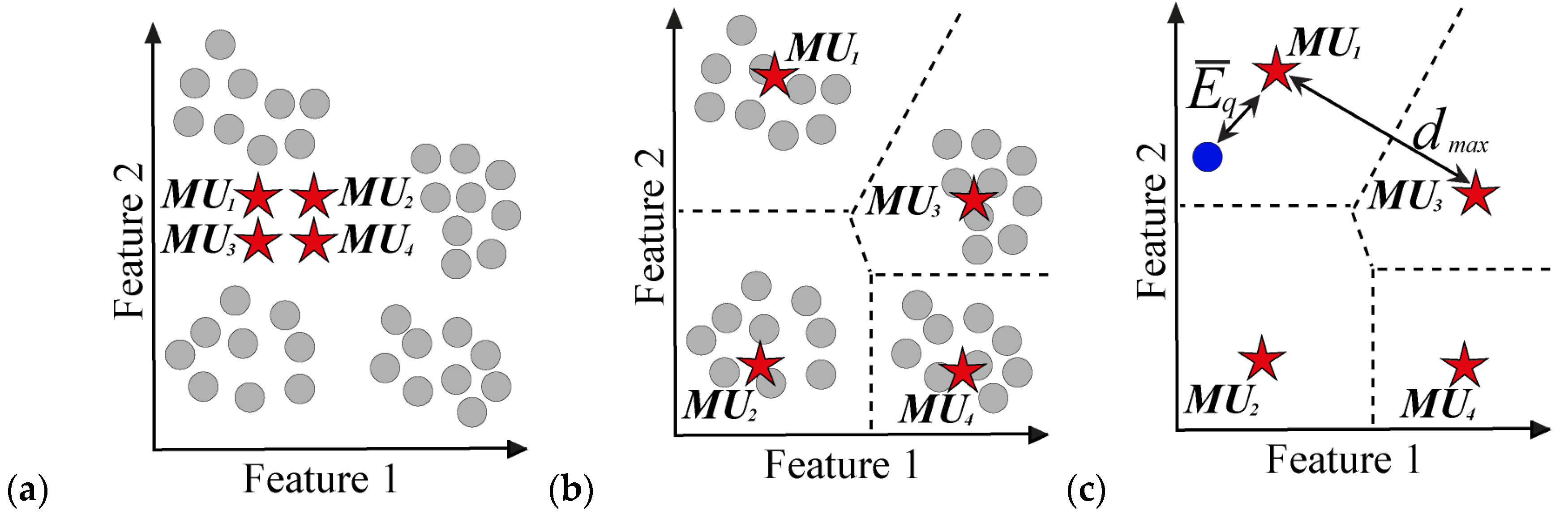
. (b) Resulting training procedure, where, the dotted lines represent the assigned memberships regions of the matching units considering Euclidian distances. The maximum distance between MUs, dmax, corresponds with MU1 and MU3. (c) Assessment of a new input data sample, Electronics 11 00287 i003. Assignation to MU1 as closest matching unit with the corresponding individual quantization error E ¯ q .
Electronics 11 00287 g002
Figure 3. Diagram of the proposed methodology based on an optimized multi-domain feature selection for the detection and classification of disturbances.
Electronics 11 00287 g003
Figure 4. Flow chart for the GA implementation.
Electronics 11 00287 g004
Figure 5. Set of different electrical signals that are synthetically generated and that belong to evaluated conditions: (a) healthy or normal, (b) sag voltage, (c) swell voltage, (d) voltage fluctuations, (e) harmonic distortion and (f) transients.
Electronics 11 00287 g005aElectronics 11 00287 g005b
Figure 6. 2-d visual representation of the data distribution for all the assessed conditions achieved by the PCA technique during the analysis of each characteristic feature matrices for: (a) the estimated features for FD and (b) the subset of selected features for FD.
Electronics 11 00287 g006
Figure 7. 2-d visual representation of the data distribution performed by the T-SNE technique over the resulting SOM neuron grid models for all considered conditions when analyzing: (a) SOM neuron grids models for TD, (b) SOM neuron grids models for FD and (c) SOM neuron grids models for TFD.
Electronics 11 00287 g007
Figure 8. 2-d visual representation of the data distribution performed by the T-SNE technique over the resulting SOM neuron grid models for all considered conditions when analyzing all SOM neuron grid models from the three analyzed domains, TD, FD and TFD.
Electronics 11 00287 g008
Figure 9. Real signal analyzed through the proposed PQ detection strategy: (a) representation of 100 s of the analyzed signal and (b) zoom over the near area where the detection of swell is presented.
Electronics 11 00287 g009
Figure 10. Achieved quantization error, E ¯ q , during the assessment of a real signal over the SOM neuron grids that models the conditions of: (a) normal condition, (b) sag, (c) swell, (d) fluctuation, (e) harmonic and (f) transients.
Electronics 11 00287 g010aElectronics 11 00287 g010b
Table 1. Mathematical models used in the generation of the synthetic signals for the 6 different conditions.
ConditionMathematical ModelParameter Description
Healthy x h l t ( k ) = A sin ( 2 π f f c k + ϕ ) + η ( k , σ ) 1 π 12 ϕ π 12
Voltage sag x s a g ( k ) = α A [ u ( k k 1 ) u ( k k 2 ) ] sin ( 2 π f f c k + ϕ ) + η ( k , σ ) 2 0.1 α 0.9
k 1 < k 2
π 12 ϕ π 12
Voltage swell x s w e l l ( k ) = α A [ u ( k k 1 ) u ( k k 2 ) ] sin ( 2 π f f c k + ϕ ) + η ( k , σ ) 0.1 α 0.3
k 1 < k 2
π 12 ϕ π 12
Transients x t r ( k ) = A [ sin ( 2 π f f c k + ϕ ) ψ ( e 750 ( k k 1 ) e 344 ( k k 1 ) ) ( u ( k k 1 ) u ( k k 2 ) ) ] + η ( k , σ ) 0.222 ψ 1.11
k b = k a + 8
π 12 ϕ π 12
Voltage fluctuation x f l ( k ) = α A sin ( 2 π f f l k + ϕ ) sin ( 2 π f f c k + ϕ ) + η ( k , σ ) 1 f f l 30
0 < α 0.1
π 12 ϕ π 12
Harmonics x h a r ( k ) = A sin ( 2 π f f c k + ϕ ) + h n = 2 M A h sin ( 2 π h n f f c k + ϕ ) + η ( k , σ ) 5 M 50
0.012 A h 0.1
π 12 ϕ π 12
1 The term η ( k , σ ) represents additive Gaussian noise with zero mean and standard deviation 0.05 σ 0.1 . 2 u (   ) is the step function.
Table 2. Proposed set of statistical features for the characterization of the available signals during the processing in the time-domain analysis, where, x(i) is a sample for i = 1, 2,…, N, and N is the number of points for each acquired signal.
Statistical Time-Domain FeatureMathematical Equation
Mean T 1 = 1 N · i = 1 N | x i |
Maximum value T 2 = m a x ( x )
Root mean square T 3 = 1 N · i = 1 N ( x i ) 2
Square root mean T 4 = ( 1 N · i = 1 N | x i | ) 2
Standard deviation T 5 = 1 N · i = 1 N ( x i T 1 ) 2
Variance T 6 = 1 N · i = 1 n ( x i T 1 ) 2
RMS shape factor T 7 = T 3 1 N · i = 1 N | x i |
SRM shape factor T 8 = T 4 1 N · i = 1 N | x i |
Crest factor T 9 = T 2 T 3
Latitude factor T 10 = T 2 T 4
Impulse factor T 11 = T 2 1 N · i = 1 N | x i |
Skewness T 12 = [ ( x i T 1 ) 3 ] T 5 3
Kurtosis T 13 = [ ( x i T 1 ) 4 ] T 5 4
Fifth moment T 14 = [ ( x i T 1 ) 5 ] T 5 5
Sixth moment T 15 = [ ( x i T 1 ) 6 ] T 5 6
Table 3. Proposed set of statistical features for the characterization of frequency spectra estimated from each available signal during its processing in the frequency-domain analysis, where s(k) is a spectrum for j = 1, 2,…, M, and M is the number of lines with fj as the frequency value of the jth spectrum line.
Statistical FeatureMathematical Equation
Mean F 1 = 1 M · j = 1 M s ( j )
Variance F 2 = 1 M 1 · j = 1 M ( s ( j ) F 1 ) 2
Third moment F 3 = 1 M ( F 2 ) 3 · j = 1 M ( s ( j ) F 1 ) 3
Fourth moment F 4 = 1 M ( F 2 ) 2 · j = 1 M ( s ( j ) F 1 ) 4
Grand mean F 5 = j = 1 M f j   s ( j ) j = 1 M s ( j )
Standard deviation 1 F 6 = j = 1 M ( f j F 5 ) 2   s ( j ) M
C factor F 7 = j = 1 M f j 2   s ( j ) j = 1 M s ( j )
D factor F 8 = j = 1 M f j 4   s ( j ) j = 1 M f j 2   s ( j )
E factor F 9 = j = 1 M f j 2   s ( j ) j = 1 M s ( j )   j = 1 M f j 4   s ( j )
G factor F 10 = F 6 F 5
Third moment 1 F 11 = j = 1 M ( f j F 5 ) 3   s ( j ) M   F 6 3
Fourth moment 1 F 12 = j = 1 M ( f j F 5 ) 4   s ( j ) M   F 6 4
H factor F 13 = j = 1 M ( f j F 5 ) 1 / 2   s ( j ) M   F 6
J factor F 14 = ( F 7 + F 8 ) F 1
Table 4. Resulting feature selection achieved by the GA–PCA selection structure applied to each evaluated condition for each analyzed domain with TD = 15, FD = 14 and TFD = 45, where, T D     TD , F D     FD and T F D     TFD .
ConditionDomain of Analysis
TDFDTFD
Normal2, 123, 1018, 19, 20, 21, 33, 34, 35, 36, 39
Sag3, 113, 64, 15, 24
Swell4, 512, 148, 32
Fluctuation5, 154, 615, 31
Harmonic2, 3, 5, 144, 521, 26
Transients4, 72, 1221, 35
Selected features2, 3, 4, 5, 7, 11, 12, 14, 152, 3, 4, 5, 6, 10, 12, 144, 8, 15, 18, 19, 20, 21, 24, 26, 31, 32, 33, 34, 35, 36, 39
Table 5. Achieved values of E ¯ q and E ¯ t resulting from the feature learning procedure performed by the proposed SOM neuron grid models.
ConditionDomain of AnalysisFusion Approach
(TD+TF+TFD)
TDFDTFD
E ¯ q E ¯ t E ¯ q E ¯ t E ¯ q E ¯ t E ¯ q E ¯ t
Healthy1.27300.02590.78890.01441.76460.02023.41770.0115
Sag9.87010.20759.93010.386281.850.3833114.5330.0951
Swell3.16490.30844.02350.109534.1350.391952.7410.2421
Flicker3.92990.09222.80750.29114.72130.175815.1050.0403
Harmonics1.09240.50430.66080.282431.66330.334337.22560.2911
Transients1.39960.07201.17450.0403485.1310.6455483.89920.6023
Table 6. Resulting feature selection achieved by the GA–PCA selection structure applied to each evaluated condition for each analyzed domain.
Feature DomainGlobal Classification Ratio
TrainingTest
TD78.7%79.3%
FD82.8%84.0%
TFD55.8%52.7%
Fusion approach (TD+TF+TFD)100%100%
Publisher’s Note: MDPI stays neutral with regard to jurisdictional claims in published maps and institutional affiliations.

