Multi-Scale Memetic Image Registration

Abstract

Many technological applications of our time rely on images captured by multiple cameras. Such applications include the detection and recognition of objects in captured images, the tracking of objects and analysis of their motion, and the detection of changes in appearance. The alignment of images captured at different times and/or from different angles is a key processing step in these applications. One of the most challenging tasks is to develop fast algorithms to accurately align images perturbed by various types of transformations. The paper reports a new method used to register images in the case of geometric perturbations that include rotations, translations, and non-uniform scaling. The input images can be monochrome or colored, and they are preprocessed by a noise-insensitive edge detector to obtain binarized versions. Isotropic scaling transformations are used to compute multi-scale representations of the binarized inputs. The algorithm is of memetic type and exploits the fact that the computation carried out in reduced representations usually produces promising initial solutions very fast. The proposed method combines bio-inspired and evolutionary computation techniques with clustered search and implements a procedure specially tailored to address the premature convergence issue in various scaled representations. A long series of tests on perturbed images were performed, evidencing the efficiency of our memetic multi-scale approach. In addition, a comparative analysis has proved that the proposed algorithm outperforms some well-known registration procedures both in terms of accuracy and runtime.

1. Introduction

The modern world uses a lot of digital imaging, both motion and static, captured through a myriad of devices of all kinds, and the trend is rapidly growing. All these images must be processed, implying understanding the content and making decisions. Most of the digital content is, in the end, irrelevant for the decision-making process but must be examined nevertheless in order to categorize it. While the human worker is still the best choice for understanding an image, the sheer amount of digital content to be processed is beyond their capabilities. Nobody can afford to hire and retain a huge army of people to analyze the digital imagery that must be processed. Besides being a huge task, it is also a repetitive and, after all, menial task, which makes it prone to errors. This is where computers can step in to perform the menial, repetitive tasks that make up the bulk of the processing and leave only final decision-making steps to humans. Even some simpler decisions can be entrusted to computers.

The understanding of digital imagery content by computers is generally referred to as “computer vision”, an umbrella term that covers all the research conducted in this field.

The processing power of computers constantly grows, but at the same time the amount of processing needed also grows, which leads to an “arms race”. Time is a critical resource and reducing the processing time is the main goal. Computers need better arms in this fight, which are materialized in better algorithms. Technological advances translate into images with higher resolution. More and more pixels are available for computers to process, but for many tasks, not all those pixels are relevant. One of the “weapons” in the arsenal is the use of lower resolution images during processing and then applying the results to the full-scale image. The lower resolution contains relevant information for the processing algorithm and limits the consumption of computing power to what matters. However, it cannot be said in advance which reduced scale is best suited for a given process. Finding a perfect balance between consumed time and quality of results can be difficult or impossible, taking too much time and thus defeating the initial goal of reducing the processing time. A way around this conundrum is the use of several reduced-scale images with various scaling factors. In the literature, this is called “multi-scale” or “pyramid strategy”, and researches indicate that it can be successfully used in multiple tasks.

This paper is structured in sections as follows. Section 2 provides a brief review of state-of-the-art works regarding multi-scale processing techniques. Section 3 summarizes the memetic approach to image registration and the algorithm we introduced in [1]. Section 4 is the main part of this article, in which we describe in detail the new method that extends the bio-inspired clustered technique presented in Section 3 to a multi-scale approach. Computation is carried out in different reduced representations to obtain promising initial solutions and identify search directions leading to the global optimum. The section also includes the computation of the search space, a justification for using multi-scale images, and the proposed methodology. The proposed algorithm was tested on various images, and the experimental results are reported in Section 5. Conclusions derived from a comparative analysis against some classical image registration methods proved the validity of the proposed algorithm, outperforming those methods from an accuracy point of view. In addition, the results show significant improvements regarding time consumption when compared to the algorithm presented in Section 3. In the last section, we summarize our conclusions and future development directions.

2. Literature Review

The idea of using multi-scaling is not new; the reasons behind it manifesting themselves early in the development of computers and computer vision. Key articles at the base of multi-scaling [2,3,4] indicate two main reasons for using images with lower resolutions in various processing stages of computer vision: first, the obvious reduction in processing power needed; second, a lower resolution eliminates distracting pixels, and thus the context of the image is better understood and can be applied on the high-resolution image.

Multi-scale images have been successfully used for various resource-intensive tasks. The identification of elements in images is one such task intensively approached. One direction looks into the identification of objects of interest in an image (salient objects), while another direction looks to identify the same object in a set of images acquired by various sources. In [5], the authors show that multi-scale images are related to the way biological vision works for segmenting, identifying objects, and understanding the perceived image.

The detection of salient segments using adapted graph algorithms and numerical techniques through multi-scale versions of an image is explored in [6]. In [7,8], Convolutional Neural Networks (CNN) are used to create models for salient object detection (objects that attract the attention of the eye) with the purpose of object detection. The CNN are trained using reduced-scale images, which provide the needed information without wasting computing time on irrelevant details. The trained network can be used to detect objects of interest in high-resolution images for various purposes, including personal identification. Multiple scale versions of an image are also used to identify targets of various sizes (both big and small) in an image through the use of the YOLO (You Only Look Once) v3 CNN in [9].

Re-identification (or identification of the same subject in multiple images) is an important task in processing images captured by various cameras. In [10], the potential of meaningful information in reduced scale images is harnessed for vehicle re-identification in images captured by non-overlapping security cameras. In [11,12], the same idea is used for the re-identification of persons. Various reduced-scale images provide useful explicit information for the stated goal. The identification of objects in static or motion images is also accomplished using multi-scale image processing in [13].

For a more engineering-based approach, multi-scale images have been used to detect and classify specific elements of importance. In [14], reduced-scale images (scale 2 and 4) are used to train a CNN to identify and outline six types of possible damages in civil infrastructure, thus relieving human inspectors of a huge workload, usually beyond their physical capabilities. An improved image denoising method that uses multi-scaling in combination with a Normalized Attention Neural Network is proposed in [15]. In [16], the authors use multi-scaling to overcome the difficulties in the detection and identification of very specific objects (ships) in single sensor images in infrared and visible spectra.

The biomedical field also benefits from the added information that can be found in reduced scale images. In [17], authors show that machine learning technology performs very well in image recognition, thus helping diagnosis, but not so well in prognosis. The authors also discuss the integration of machine learning with multi-scale modelling to improve prognosis performance.

3. Memetic Approach of Image Registration

Hybrid and memetic algorithms are among the most commonly used metaheuristics for image alignment, as the evolutionary process is enhanced with local search techniques that reduce the risk of premature convergence and speed up computation. In the following, we present the basic method we proposed in [1]. The method will be further improved to speed up computation, extending it to multi-scale processing and including specialized mechanisms to avoid premature convergence.

The degradation model is of geometric type, consisting of translations, rotations, and non-uniform scaling. We denote the target image by T and let S be the observed image, i.e., the perturbed version of T, where

$$\mathrm{S}\left(\mathrm{x},\mathrm{y}\right)=\mathrm{T}\left({\mathrm{f}}_{\mathrm{p}}\left(\mathrm{x},\mathrm{y}\right)\right)$$

(1)

and

$${\mathrm{f}}_{\mathrm{p}}\left(\mathrm{x},\mathrm{y}\right)=\left[\begin{array}{c}\mathrm{a}\\ \mathrm{b}\end{array}\right]+\left[\begin{array}{cc}{\mathrm{s}}_{\mathrm{x}}& 0\\ 0& {\mathrm{s}}_{\mathrm{y}}\end{array}\right]·\left[\begin{array}{cc}\cos \mathsf{\theta }& -\sin \mathsf{\theta }\\ \sin \mathsf{\theta }& \cos \mathsf{\theta }\end{array}\right]·\left[\begin{array}{c}\mathrm{x}\\ \mathrm{y}\end{array}\right].$$

(2)

The parameter vector defining (2) is $\mathrm{p}=\left(\mathrm{a},\mathrm{b},{\mathrm{s}}_{\mathrm{x}},{\mathrm{s}}_{\mathrm{y}},\mathsf{\theta }\right)$, where (a, b) is the translation vector, ${\mathrm{s}}_{\mathrm{x}}$ and ${\mathrm{s}}_{\mathrm{y}}$ are the scale factors, ${\mathrm{s}}_{\mathrm{x}},{\mathrm{s}}_{\mathrm{y}}>0$, and $\mathsf{\theta }$ is the rotation angle. Note that the rotation is relative to the upper left corner of the image. From a mathematical point of view, aligning S to T means computing g, the transformation to reverse (2), that is:

$$\mathrm{T}\left(\mathrm{x},\mathrm{y}\right)=\mathrm{S}\left({\mathrm{g}}_{\mathrm{p}}\left(\mathrm{x},\mathrm{y}\right)\right).$$

(3)

The inverse transformation ${\mathrm{g}}_{\mathrm{p}}$ is computed as:

$${\mathrm{g}}_{\mathrm{p}}\left(\mathrm{x},\mathrm{y}\right){=\mathrm{R}}^{\mathrm{T}}·{\mathrm{S}}_{\mathrm{xy}}^{-1}\left(\left[\begin{array}{c}\mathrm{x}\\ \mathrm{y}\end{array}\right]-\left[\begin{array}{c}\mathrm{a}\\ \mathrm{b}\end{array}\right]\right)$$

(4)

where ${\mathrm{S}}_{\mathrm{xy}}^{-1}=\left[\begin{array}{cc}\frac{1}{{\mathrm{s}}_{\mathrm{x}}}& 0\\ 0& \frac{1}{{\mathrm{s}}_{\mathrm{y}}}\end{array}\right]$ and $\mathrm{R}=\left[\begin{array}{cc}\cos \mathsf{\theta }& -\sin \mathsf{\theta }\\ \sin \mathsf{\theta }& \cos \mathsf{\theta }\end{array}\right]$.

To solve the image alignment problem using evolutionary computing one has to define the chromosome representation, the search space, and the fitness function. In our work, the images are binarized by applying an edge detector. The chromosome space coincides with the phenotype space, and it is defined by $\left[{\mathrm{a}}_{\min },{\mathrm{a}}_{\max }\right]\times \left[{\mathrm{b}}_{\min },{\mathrm{b}}_{\max }\right]\times \left[-\mathsf{\pi },0\right]\times (0,{\mathrm{smax}}_{\mathrm{x}}]\times (0,{\mathrm{smax}}_{\mathrm{y}}]$. The boundaries of the translation parameters are evaluated based on ${\mathrm{smax}}_{\mathrm{x}}$, ${\mathrm{smax}}_{\mathrm{y}}$, and the object pixels in T and S, respectively [1]. The quality of a chromosome corresponding to a parameter vector p1 is defined in our work by the Dice similarity between the target and the result computed by (3):

$$\mathrm{fitness}\left(\mathrm{p}1\right)=\mathrm{DICE}\left(\mathrm{S}\left({\mathrm{g}}_{\mathrm{p}1}\right),\mathrm{T}\right).$$

(5)

The Dice coefficient of the binary images $\mathrm{A}$ and $\mathrm{B}$ is defined by [18]:

$$\mathrm{DICE}\left(\mathrm{A},\mathrm{B}\right)=\frac{2·\left|\mathrm{A}{\displaystyle \cap }\mathrm{B}\right|}{\left|\mathrm{A}\right|+\left|\mathrm{B}\right|}$$

(6)

where $|·|$ is the cardinal function.

The registration mechanism combines a version of Firefly Algorithm (FA) global optimization [19,20] with the local search implemented by Two Membered Evolutionary Strategy (2MES) [21] applied on clustered data. Let ${\mathrm{c}}_0$ be an input individual, and we denote the initial step size by ${\mathsf{\sigma }}_0$. At each moment t, 2MES iteratively updates the point ${\mathrm{c}}_{\mathrm{t}-1}$ using,

$${\mathrm{c}}_{\mathrm{t}}=\{\begin{array}{ll}\hfill {\mathrm{c}}_{\mathrm{t}-1}+\mathrm{z},& \mathrm{if}\mathrm{fitness}\left({\mathrm{c}}_{\mathrm{t}-1}+\mathrm{z}\right)>\mathrm{fitness}\left({\mathrm{c}}_{\mathrm{t}-1}\right)\\ \hfill {\mathrm{c}}_{\mathrm{t}-1},& \mathrm{otherwise}\end{array}$$

(7)

where $\mathrm{z}$ is a random value drawn from $\mathrm{N}\left(0,{\mathsf{\sigma }}_{\mathrm{t}-1}\right)$. The step size parameter ${\mathsf{\sigma }}_{\mathrm{t}}$ is updated according to the celebrated 1/5 rule [21].

$${\mathsf{\sigma }}_{\mathrm{t}}=\{\begin{array}{cc}\frac{{\mathsf{\sigma }}_{\mathrm{t}-1}}{\mathsf{\vartheta }},& \mathrm{sr}>0.2\\ {\mathsf{\sigma }}_{\mathrm{t}-1}·\mathsf{\vartheta },& \mathrm{sr}<0.2\\ {\mathsf{\sigma }}_{\mathrm{t}-1},& \mathrm{sr}=0.2\end{array} ,$$

(8)

where $\mathsf{\vartheta }\in [0.817,1)$ and $\mathrm{sr}$ is the success rate, i.e., the displacement rate corresponding to the last $\mathsf{\tau }$ updates.

FA is a nature-inspired search that simulates the behavior of fireflies in terms of bioluminescence evolution. The position of a firefly corresponds to a candidate solution of (1), its fitness being measured by the corresponding light intensity. Each firefly j attracts less bright fireflies i, i.e., j modifies the positions ${\mathrm{c}}_{\mathrm{i}}$ according to:

$${\mathrm{c}}_{\mathrm{i}}\left(\mathrm{t}+1\right){=\mathrm{c}}_{\mathrm{i}}\left(\mathrm{t}\right){+\mathsf{\beta }}_{\mathrm{j}}\left(\mathrm{r}\right)·\left({\mathrm{c}}_{\mathrm{j}}\left(\mathrm{t}\right){-\mathrm{c}}_{\mathrm{i}}\left(\mathrm{t}\right)\right)+\mathsf{\alpha }\mathrm{r}·\mathsf{\epsilon },$$

(9)

where $\mathsf{\alpha }\mathrm{r}$ is the randomness parameter, $\mathsf{\epsilon }$ is a draw from $\mathrm{U}\left(0,1\right)$, ${\mathsf{\beta }}_{\mathrm{j}}\left(\mathrm{r}\right)$is the attractiveness of firefly j seen by firefly i. The attractiveness function is defined as:

$${\mathsf{\beta }}_{\mathrm{j}}\left(\mathrm{r}\right){=\mathsf{\beta }}_0·{\mathrm{e}}^{{-\mathsf{\gamma }\mathrm{r}}^2}$$

(10)

where $\mathrm{r}$ is the distance between fireflies i and j, ${\mathsf{\beta }}_0$ indicates the brightness at $\mathrm{r}=0,$ and $\mathsf{\gamma }$ stands for the light absorption coefficient. In our work, we use $\mathsf{\alpha }\mathrm{r}$, the updating rule, and the border reflection mechanism introduced in [22].

The registration algorithm reported in [1] is summarized below as Algorithm 1, where the FA parameters are ${\mathsf{\beta }}_0,\mathsf{\gamma }$, the 2MES input arguments are ${\mathsf{\sigma }}_0,\mathsf{\vartheta },$ $\mathsf{\tau }$, and the size of the sequence of individuals, MAX.

Algorithm 1 Cluster-Based Memetic Algorithm
1.	Input: the binarized versions of S and T, 2MES parameters, FA parameters, the number of iterations NMax, K (K < Nmax), and the fitness value threshold ${\mathsf{\tau }}_{\mathrm{stop}}$
2.	Compute the boundaries of the search space
3.	Compute the initial population, randomly generate the candidate solutions, and apply the 2MES procedure to locally improve a small number of individuals
4.	Evaluate the initial population and find the best; time = 0
5.	while $\mathrm{time}<\mathrm{NMax}$ and the highest fitness value ${<\mathsf{\tau }}_{\mathrm{stop}}$ do
6.	Execute one FA iteration
7.	Compute the best individual
8.	if the best fitness value has not been improved
9.	if the best fitness value has not been improved during the last K iterations, apply the premature convergence avoidance mechanism:
10.	Increase the step size of 2MES,
11.	Increase the number of clusters
12.	Replace a small number of individuals with randomly generated and locally improved ones
13.	end if
14.	Apply k-means to split the population into clusters and locally improve the best individual from each class using 2MES
15.	Keep the best individual in the current population
16.	end if
17.	$\mathrm{time}=\mathrm{time}+1$
18.	end while
19.	Output: The best individual corresponding to the perturbation parameter vector

4. The New Multi-Scale Methodology

The algorithm aligns an observed image S to the target T by extending the bio-inspired cluster-based technique described in S3 to a multi-scale approach that includes mechanisms especially tailored to avoid premature convergence. The ideas underlying the proposed methodology are that the computation carried out in different reduced representations can produce both promising initial solutions and individuals able to redirect the search to the global optimum. Furthermore, multi-scale processing may significantly improve registration accuracy and lead to faster algorithms.

4.1. The Geometric Degradation Model and the Search Space

The proposed approach aims to register images perturbed by translations, rotations, and non-uniform scaling according to (1). The translation domain $\left[{\mathrm{a}}_{\min },{\mathrm{a}}_{\max }\right]\times \left[{\mathrm{b}}_{\min },{\mathrm{b}}_{\max }\right]$ can be narrowed down by considering the following transformation instead of (2).

$${\mathrm{f}}_{\mathrm{p}}\left(\mathrm{x},\mathrm{y}\right)=\left[\begin{array}{c}\mathrm{m}\\ \mathrm{n}\end{array}\right]+\left[\begin{array}{c}\mathrm{a}\\ \mathrm{b}\end{array}\right]+\left[\begin{array}{cc}{\mathrm{s}}_{\mathrm{x}}& 0\\ 0& {\mathrm{s}}_{\mathrm{y}}\end{array}\right]·\left[\begin{array}{cc}\cos \mathsf{\theta }& -\sin \mathsf{\theta }\\ \sin \mathsf{\theta }& \cos \mathsf{\theta }\end{array}\right]·\left[\begin{array}{c}\mathrm{x}-\mathrm{m}\\ \mathrm{y}-\mathrm{n}\end{array}\right],$$

(11)

where $\mathrm{p}=\left(\mathrm{a},\mathrm{b},{\mathrm{s}}_{\mathrm{x}},{\mathrm{s}}_{\mathrm{y}},\mathsf{\theta }\right)$ and the rotation is relative to the center of the image (m, n). In this case, the inverse transformation ${\mathrm{g}}_{\mathrm{p}}$ is given by:

$${\mathrm{g}}_{\mathrm{p}}\left(\mathrm{x},\mathrm{y}\right)=\left[\begin{array}{c}\mathrm{m}\\ \mathrm{n}\end{array}\right]+{\mathrm{R}}^{\mathrm{T}}·{\mathrm{S}}_{\mathrm{xy}}^{-1}\left(\left[\begin{array}{c}\mathrm{x}\\ \mathrm{y}\end{array}\right]-\left[\begin{array}{c}\mathrm{a}+\mathrm{m}\\ \mathrm{b}+\mathrm{n}\end{array}\right]\right).$$

(12)

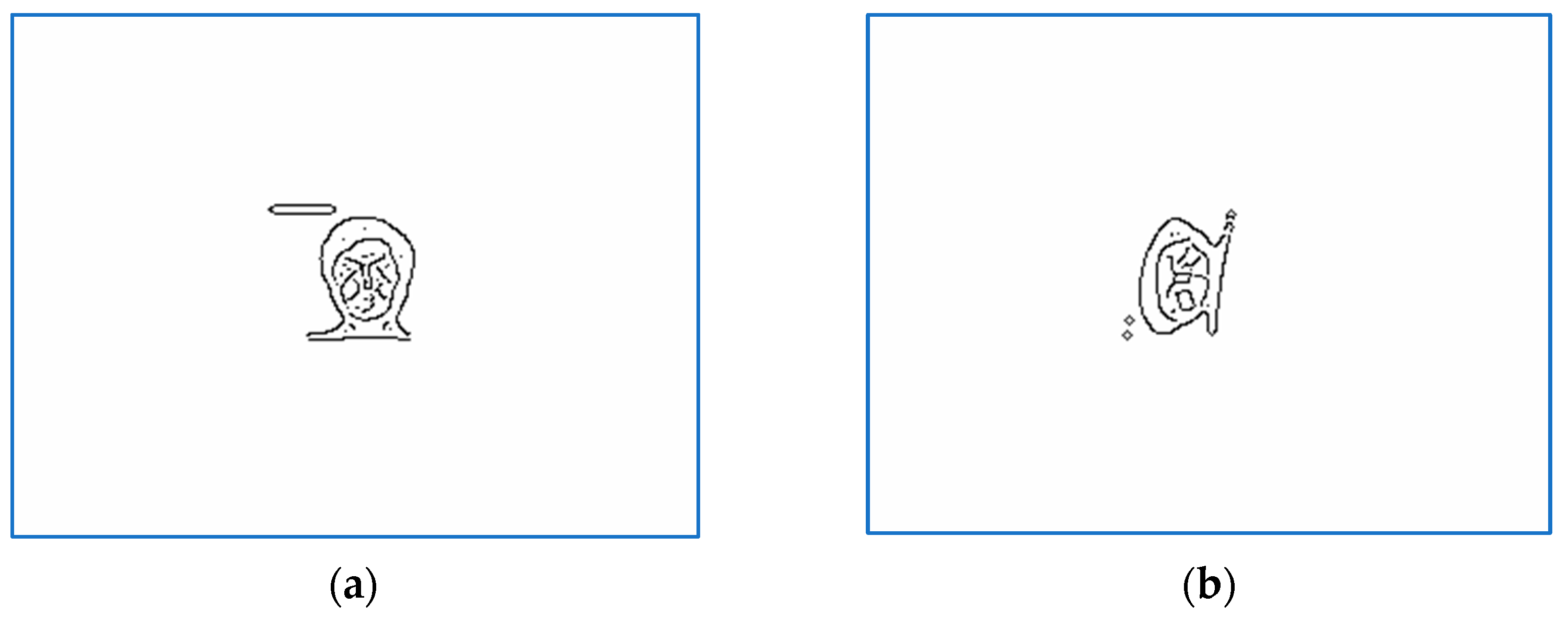
The search space boundaries are set as follows. We assume that $\left(\mathsf{\theta },{\mathrm{s}}_{\mathrm{x}},{\mathrm{s}}_{\mathrm{y}}\right)\in \left[-\mathsf{\pi }/2,0\right]\times \left[0,{\mathrm{smax}}_{\mathrm{x}}\right]\times \left[0,{\mathrm{smax}}_{\mathrm{y}}\right]$. The alignment is performed using a binarized version of S and T computed by the Canny edge detector [23]; therefore, the input images are represented by sets of contour pixels. We denote by $\mathrm{B}\left(\mathrm{T}\right)=\left\{\left({\mathrm{x}}_{\mathrm{T}},{\mathrm{y}}_{\mathrm{T}}\right),{\mathrm{minx}}_{\mathrm{T}}\le {\mathrm{x}}_{\mathrm{T}}\le {\mathrm{maxx}}_{\mathrm{T}},{\mathrm{miny}}_{\mathrm{T}}\le {\mathrm{y}}_{\mathrm{T}}\le {\mathrm{maxy}}_{\mathrm{T}}\right\}$ and $\mathrm{B}\left(\mathrm{S}\right)=\left\{\left({\mathrm{x}}_{\mathrm{S}},{\mathrm{y}}_{\mathrm{S}}\right),{\mathrm{minx}}_{\mathrm{S}}\le {\mathrm{x}}_{\mathrm{S}}\le {\mathrm{maxx}}_{\mathrm{S}},{\mathrm{miny}}_{\mathrm{S}}\le {\mathrm{y}}_{\mathrm{S}}\le {\mathrm{maxy}}_{\mathrm{S}}\right\}$ the binarized versions of T and S, respectively. Since the elements in B(S) are obtained from those in B(T) using (11), we obtain:

$${\mathrm{minx}}_{\mathrm{T}}\le \mathrm{m}+\mathrm{a}+{\mathrm{s}}_{\mathrm{x}}·\left(\left(\mathrm{x}-\mathrm{m}\right)·\cos \mathsf{\theta }-\left(\mathrm{y}-\mathrm{n}\right)·\sin \mathsf{\theta }\right)\le {\mathrm{maxx}}_{\mathrm{T}}$$

And

$${\mathrm{miny}}_{\mathrm{T}}\le \mathrm{n}+\mathrm{b}+{\mathrm{s}}_{\mathrm{y}}·\left(\left(\mathrm{x}-\mathrm{m}\right)·\sin \mathsf{\theta }+\left(\mathrm{y}-\mathrm{n}\right)·\cos \mathsf{\theta }\right)\le {\mathrm{maxy}}_{\mathrm{T}}.$$

By straightforward computation, we obtain that $\left(\mathrm{a},\mathrm{b}\right)\in \left[{\mathrm{a}}_{\min },{\mathrm{a}}_{\max }\right]\times \left[{\mathrm{b}}_{\min },{\mathrm{b}}_{\max }\right]$:

$${\mathrm{a}}_{\min }={\mathrm{minx}}_{\mathrm{T}}-\mathrm{m}+\underset{\left(\mathrm{x},\mathrm{y},\mathsf{\theta },{\mathrm{s}}_{\mathrm{x}}\right)\in \mathrm{Da}}{\min }\mathrm{a}\_\lim \left(\mathrm{x},\mathrm{y},\mathsf{\theta },{\mathrm{s}}_{\mathrm{x}}\right),$$

(13)

$${\mathrm{a}}_{\max }={\mathrm{maxx}}_{\mathrm{T}}-\mathrm{m}+\underset{\left(\mathrm{x},\mathrm{y},\mathsf{\theta },{\mathrm{s}}_{\mathrm{x}}\right)\in \mathrm{Da}}{\max }\mathrm{a}\_\lim \left(\mathrm{x},\mathrm{y},\mathsf{\theta },{\mathrm{s}}_{\mathrm{x}}\right),$$

(14)

$${\mathrm{b}}_{\min }={\mathrm{miny}}_{\mathrm{T}}-\mathrm{n}+\underset{\left(\mathrm{x},\mathrm{y},\mathsf{\theta },{\mathrm{s}}_{\mathrm{y}}\right)\in \mathrm{Db}}{\min }\mathrm{b}\_\lim \left(\mathrm{x},\mathrm{y},\mathsf{\theta },{\mathrm{s}}_{\mathrm{y}}\right),$$

(15)

$${\mathrm{b}}_{\max }={\mathrm{maxy}}_{\mathrm{T}}-\mathrm{n}+\underset{\left(\mathrm{x},\mathrm{y},\mathsf{\theta },{\mathrm{s}}_{\mathrm{y}}\right)\in \mathrm{Db}}{\max }\mathrm{b}\_\lim \left(\mathrm{x},\mathrm{y},\mathsf{\theta },{\mathrm{s}}_{\mathrm{y}}\right),$$

(16)

where

$$\begin{gathered} \mathrm{a}\_\lim :\mathrm{Da}\to ℝ \\ \mathrm{Da}=\left[-\mathsf{\pi }/2,0\right]\times \left[0,{\mathrm{smax}}_{\mathrm{x}}\right]\times \left[{\mathrm{minx}}_{\mathrm{S}},{\mathrm{maxx}}_{\mathrm{S}}\right]\times \left[{\mathrm{miny}}_{\mathrm{S}},{\mathrm{maxy}}_{\mathrm{S}}\right] \\ \mathrm{a}\_\lim \left(\mathrm{x},\mathrm{y},\mathsf{\theta },{\mathrm{s}}_{\mathrm{x}}\right){=\mathrm{s}}_{\mathrm{x}}·\left(\left(\mathrm{y}-\mathrm{n}\right)·\sin \mathsf{\theta }-\left(\mathrm{x}-\mathrm{m}\right)·\cos \mathsf{\theta }\right) \end{gathered}$$

(17)

And

$$\begin{gathered} \mathrm{b}\_\lim :\mathrm{Db}\to ℝ \\ \mathrm{Db}=\left[-\mathsf{\pi }/2,0\right]\times \left[0,{\mathrm{smax}}_{\mathrm{y}}\right]\times \left[{\mathrm{minx}}_{\mathrm{S}},{\mathrm{maxx}}_{\mathrm{S}}\right]\times \left[{\mathrm{miny}}_{\mathrm{S}},{\mathrm{maxy}}_{\mathrm{S}}\right] \\ \mathrm{b}\_\lim \left(\mathrm{x},\mathrm{y},\mathsf{\theta },{\mathrm{s}}_{\mathrm{y}}\right){=-\mathrm{s}}_{\mathrm{y}}·\left(\left(\mathrm{x}-\mathrm{m}\right)·\sin \mathsf{\theta }+\left(\mathrm{y}-\mathrm{n}\right)·\cos \mathsf{\theta }\right) \end{gathered}$$

(18)

Note that the functions $\mathrm{a}\_\lim$ and $\mathrm{b}\_\lim$ are bounded and attain their margins. From a practical point of view, the extreme values of $\mathrm{a}\_\lim$ and $\mathrm{b}\_\lim$ can be computed in many ways. In our work, we used the pattern search method implemented by the MATLAB function patternsearch [24].

4.2. The Multi-Scale Representation of Images

A long series of research works involving multi-scale image processing using various mathematical tools have been reported in the literature [2,3,4,5,6,7,8,9,10,11,12,13,14,15,16,17]. In our approach, scaling refers to the uniform change of object sizes in processed images and corresponds to the standard geometric transformation (11) defined by the parameter vector ${\mathrm{p}}_{\mathrm{s}}=\left(0,0,\mathrm{s},\mathrm{s},0\right),\mathrm{s}>1$. 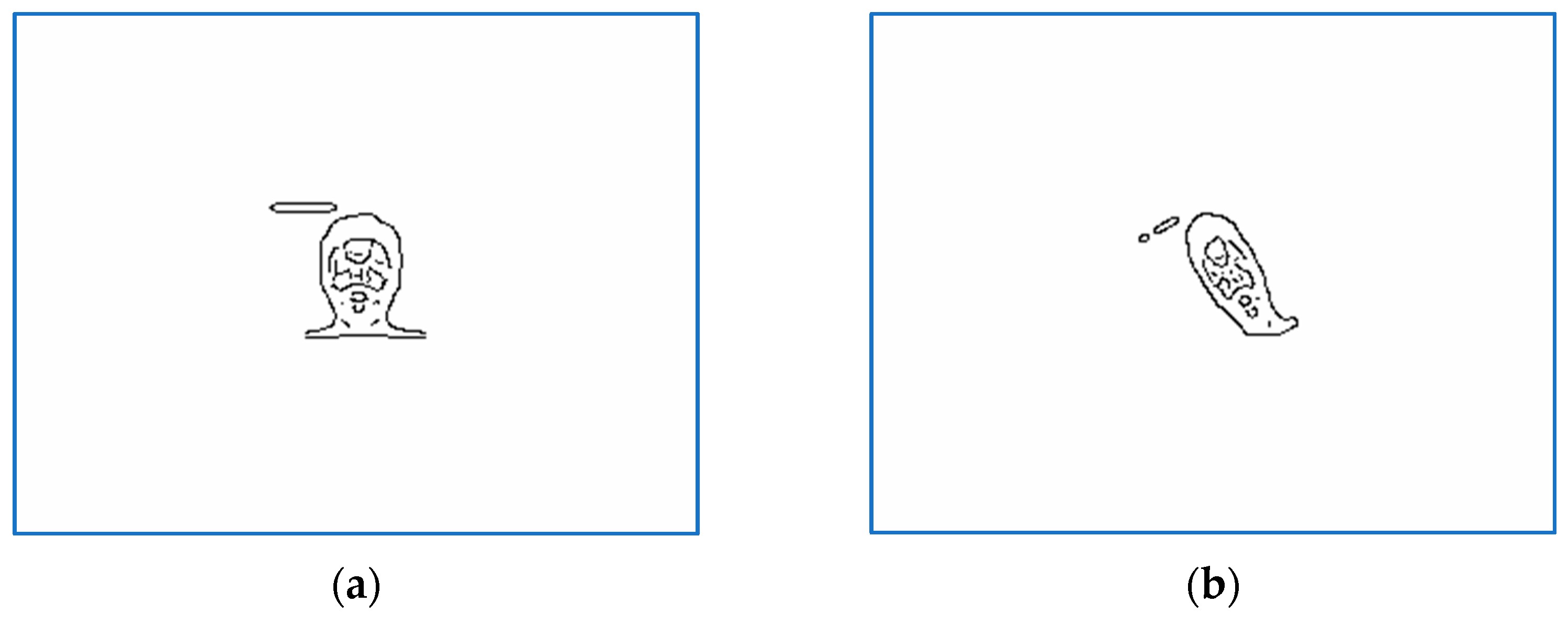Note that the dimension of the input images remains unchanged, while the size of the binary representations $\mathrm{B}\left(\mathrm{T}\right)$ and $\mathrm{B}\left(\mathrm{S}\right)$ decrease proportionally to s.

Let $\mathrm{s}>1$ be a stretching factor, T the target image, S the version of T perturbed by (11) with $\mathrm{p}=\left(\mathrm{a},\mathrm{b},{\mathrm{s}}_{\mathrm{x}},{\mathrm{s}}_{\mathrm{y}},\mathsf{\theta }\right),$ and $\left[{\mathrm{a}}_{\min },{\mathrm{a}}_{\max }\right]\times \left[{\mathrm{b}}_{\min },{\mathrm{b}}_{\max }\right]\times \left[-\mathsf{\pi }/2,0\right]\times (0,{\mathrm{smax}}_{\mathrm{x}}]\times (0,{\mathrm{smax}}_{\mathrm{y}}]$ the search space corresponding to the inputs S and T. The representation of S and T in scale s, denoted by ${\mathrm{S}}^{\mathrm{s}}$ and ${\mathrm{T}}^{\mathrm{s}}$, leads to a narrowed search space $\left[{\mathrm{a}}_{\min }/\mathrm{s},{\mathrm{a}}_{\max }/\mathrm{s}\right]\times \left[{\mathrm{b}}_{\min }/\mathrm{s},{\mathrm{b}}_{\max }/\mathrm{s}\right]\times \left[-\mathsf{\pi }/2,0\right]\times (0,{\mathrm{smax}}_{\mathrm{x}}]\times (0,{\mathrm{smax}}_{\mathrm{y}}]$. Indeed, denoting by ${\mathrm{p}}^{\prime }=\left(\mathrm{a}/\mathrm{s},\mathrm{b}/\mathrm{s},{\mathrm{s}}_{\mathrm{x}},{\mathrm{s}}_{\mathrm{y}},\mathsf{\theta }\right)$, we obtain:

$$\begin{gathered} {\mathrm{S}}^{\mathrm{s}}\left(\mathrm{x},\mathrm{y}\right)=\mathrm{S}\left({\mathrm{f}}_{{\mathrm{p}}_{\mathrm{s}}}\left(\mathrm{x},\mathrm{y}\right)\right)=\mathrm{T}\left({\mathrm{f}}_{\mathrm{p}}\left({\mathrm{f}}_{{\mathrm{p}}_{\mathrm{s}}}\left(\mathrm{x},\mathrm{y}\right)\right)\right) \\ {\mathrm{f}}_{\mathrm{p}}\left({\mathrm{f}}_{{\mathrm{p}}_{\mathrm{s}}}\left(\mathrm{x},\mathrm{y}\right)\right)={\mathrm{f}}_{{\mathrm{p}}_{\mathrm{s}}}\left({\mathrm{f}}_{{\mathrm{p}}^{\prime }}\left(\mathrm{x},\mathrm{y}\right)\right) \end{gathered}$$

(19)

Since ${\mathrm{T}}^{\mathrm{s}}\left(\mathrm{x},\mathrm{y}\right)=\mathrm{T}\left({\mathrm{f}}_{{\mathrm{p}}_{\mathrm{s}}}\left(\mathrm{x},\mathrm{y}\right)\right)$, the following relation holds:

$${\mathrm{S}}^{\mathrm{s}}\left(\mathrm{x},\mathrm{y}\right){=\mathrm{T}}^{\mathrm{s}}\left({\mathrm{f}}_{{\mathrm{p}}^{\prime }}\left(\left(\mathrm{x},\mathrm{y}\right)\right)\right)$$

(20)

Consequently, aligning S to T can be reduced to registering ${\mathrm{S}}^{\mathrm{s}}$ and ${\mathrm{T}}^{\mathrm{s}}$. That is, computing p’.

From an implementation point of view, digital image scaling using large scale factors s involves information loss due to object shrinkage. Therefore, the size of the binary representations $\mathrm{B}\left({\mathrm{T}}^{\mathrm{s}}\right)$ and $\mathrm{B}\left({\mathrm{S}}^{\mathrm{s}}\right)$ is smaller than the size of $\mathrm{B}\left(\mathrm{T}\right)$ and $\mathrm{B}\left(\mathrm{S}\right)$, yielding to faster registration algorithms.

The multi-scale memetic algorithm introduced in the next section involves stages that use images represented at different scale factors. The algorithm evolves from one stage to another by changing the chromosome values and the boundaries of the translation parameter according to (20).

4.3. The Proposed Multi-Scale Registration Method

The extension of the clustered-based memetic algorithm provided in S3 registers pairs of monochrome images (S, T) in the case of the perturbation model defined by (11). If S and T are colored images, monochrome representation can be considered instead to obtain the inverse transformation (11).

The proposed algorithm involves a pre-processing stage, as follows. First, the binary representations B(S) and B(T) are computed using a noise invariant edge detector, and the search space boundaries are evaluated according to (13)–(16). Then, the data is represented at two scales $1<\mathrm{s}1<\mathrm{s}2$. The scale s1 is used in developing the registration procedure from (Algorithm 2), while s2 is used to generate the initial population (Algorithm 3) and to avoid getting stuck in a local optimum (Algorithm 4). The genotypes computed in the search space defined by s2 are converted in the algorithm’s scale s1 using transformation (2), where $\mathrm{s}=\mathrm{s}1/\mathrm{s}2$. One can generalize the multi-scale approach by using multiple scale parameters to develop Algorithms 3 and 4, respectively. The fitness function that controls the evolution of the memetic algorithm is defined by (6), while the method used to cluster the current population of individuals is the k-mean. Note that the fitness values lie in [0, 1].

First, the population is randomly instantiated. Then, a few chromosomes computed by Algorithm 1 using the s2 scale are added to it. The memetic registration is an iterative process that applies an FA iteration to compute the new generation followed by locally 2MES-based improvement of the best chromosome of clustered data. The data is grouped into k clusters, which varies depending on the population quality.

$$\mathrm{k}={\mathrm{c}}_{\mathrm{number}}+\frac{\mathrm{ct}1}{\mathrm{bvalFA}},$$

(21)

where $\mathrm{ct}1>1$ is a constant that controls the maximum number of clusters, and c_number stands for the initial number of clusters.

To avoid premature convergence, we apply the following procedure. If the best fitness value bval is the same during the last iterations, increase the step size of 2MES, multiplying it by $\mathrm{ct}2/{\mathrm{bval}}^2,$ where $\mathrm{ct}2>1$ is a constant tuning the perturbation size z in (7). If the best fitness value bval is the same during the last it’ > it iterations, ${\mathrm{k}}_0$ new locally improved individuals and the result computed by Algorithm 1 with $\mathrm{s}2=15$ replace ${\mathrm{k}}_0+1$ individuals belonging to the current population.

The proposed method is summarized by Algorithm 2. Using ${\mathrm{C}\text{\_}\mathrm{Pop}}^{\mathrm{t}}{=\{\mathrm{c}}_1^{\mathrm{t}}{,\mathrm{c}}_2^{\mathrm{t}}{,\dots ,\mathrm{c}}_{\mathrm{n}}^{\mathrm{t}}\}$, we denote the population at moment t. The input arguments are grouped depending on their use, as follows:

• general parameters: the input images, S and T; the maximum number of iterations, NMax; the population size, n; the threshold fitness value, ${\mathsf{\tau }}_{\mathrm{stop}}$; the scales s1 and s2; the constants c_number, ct1, and ct2; 2MES inputs, ${{\mathsf{\sigma }}^{\prime }}_0$, ${\mathsf{\vartheta }}^{\prime },{{\mathsf{\tau }}^{\prime }}_{\mathrm{ES}},$ and ${\mathrm{MAX}}^{\prime }$; FA parameters ${\mathsf{\beta }}_0,\mathsf{\gamma }$;
• Algorithm 3 parameters, corresponding to Algorithm 1 arguments: 2MES parameters, ${\mathsf{\sigma }}_0,\mathsf{\vartheta }{,\mathsf{\tau }}_{\mathrm{ES}},\mathsf{\upsilon },$ and MAX; FA parameters (same as those belonging to the list of general parameters); NMax1, K1, and the threshold value ${\mathsf{\tau }}_{\mathrm{stop}1}$;
• Algorithm 4 parameters: the number of non-effective successive iterations, i.e., without highest quality changes, cp; it, it’, and ${\mathrm{k}}_0$ as described above; 2MES parameters (same as those belonging to the list of general parameters); Algorithm 1 parameters (same as those described in the list of Algorithm 3 parameters); the population C_Pop.

Algorithm 2 Multi-Scale Memetic Algorithm
1.	Input:$\mathrm{S}$, $\mathrm{T}$, $\mathrm{NMAX}$, $\mathrm{n}$, ${\mathsf{\tau }}_{\mathrm{stop}}$, $\mathrm{s}1$, $\mathrm{s}2$, ${{\mathsf{\sigma }}^{\prime }}_0$, ${\mathsf{\vartheta }}^{\prime }$, ${{\mathsf{\tau }}^{\prime }}_{\mathrm{ES}}$, ${\mathsf{\upsilon }}^{\prime }$, ${\mathrm{MAX}}^{\prime }$, ${\mathsf{\beta }}_0$, $\mathsf{\gamma }$, ${\mathsf{\sigma }}_0$, $\mathsf{\vartheta }$, ${\mathsf{\tau }}_{\mathrm{ES}}$, $\mathsf{\upsilon }$, $\mathrm{MAX}$, $\mathrm{NMAX}1$, $\mathrm{K}1$, ${\mathsf{\tau }}_{\mathrm{stop}1}$
2.	Compute $\mathrm{B}\left({\mathrm{T}}^{\mathrm{s}1}\right)$, $\mathrm{B}\left({\mathrm{T}}^{\mathrm{s}2}\right)$, $\mathrm{B}\left({\mathrm{S}}^{\mathrm{s}1}\right)$, $\mathrm{B}\left({\mathrm{S}}^{\mathrm{s}2}\right)$, and the corresponding boundaries of each search space
3.	$\mathrm{t}=0;\mathrm{cp}=0$
4.	Compute $\mathrm{C}\_{\mathrm{Pop}}^{\mathrm{t}}$ using Algorithm 3 and the input arguments $\mathrm{n}$, $\mathrm{B}\left({\mathrm{T}}^{\mathrm{s}2}\right)$, $\mathrm{B}\left({\mathrm{S}}^{\mathrm{s}2}\right)$, ${\mathsf{\sigma }}_0$, ${\mathsf{\vartheta }}_0$, ${\mathsf{\tau }}_{\mathrm{ES}0}$, $\mathsf{\upsilon }$, $\mathrm{MAX}$, ${\mathsf{\beta }}_0$, $\mathsf{\gamma }$, $\mathrm{NMAX}1$, $\mathrm{K}1,$ and ${\mathsf{\tau }}_{\mathrm{stop}1}$
5.	Obtain the representation of $\mathrm{C}\_{\mathrm{Pop}}^{\mathrm{t}}$ in the s1 scale search space
6.	Evaluate $\mathrm{C}\_{\mathrm{Pop}}^{\mathrm{t}}$ and compute $\mathrm{bval}=\underset{\mathrm{c}\in {\mathrm{C}\text{\_}\mathrm{Pop}}^{\mathrm{t}}}{\max }\mathrm{fitness}\left(\mathrm{c}\right)$
7.	while$\mathrm{t}<\mathrm{NMax}$ and ${\mathrm{bval}<\mathsf{\tau }}_{\mathrm{stop}}$ do
8.	Apply an FA iteration and get $\mathrm{C}\_{\mathrm{Pop}}^{\mathrm{t}+1}$
9.	Compute $\mathrm{bindFA}$: $\mathrm{bvalFA}=\underset{\mathrm{c}\in {\mathrm{C}\text{\_}\mathrm{Pop}}^{\mathrm{t}+1}}{\max }\mathrm{fitness}\left(\mathrm{c}\right)$
10.	if $\mathrm{bvalFA}\le \mathrm{bval}$
11.	Apply the premature convergence avoiding mechanism Algorithm 4 with the input arguments $\mathrm{n}$, $\mathrm{B}\left({\mathrm{T}}^{\mathrm{s}2}\right)$, $\mathrm{B}\left({\mathrm{S}}^{\mathrm{s}2}\right)$, $\mathrm{cp}$, $\mathrm{it}$, ${\mathrm{it}}^{\prime }$, ${\mathrm{k}}_0$, ${{\mathsf{\sigma }}^{\prime }}_0$, ${\mathsf{\vartheta }}^{\prime }$, ${{\mathsf{\tau }}^{\prime }}_{\mathrm{ES}}$, ${\mathrm{MAX}}^{\prime }$, ${\mathsf{\sigma }}_0$, ${\mathsf{\vartheta }}_0$, ${\mathsf{\tau }}_{\mathrm{ES}0}$, $\mathsf{\upsilon }$, $\mathrm{MAX}$, ${\mathsf{\beta }}_0$, $\mathsf{\gamma }$, $\mathrm{NMAX}1$, $\mathrm{K}1$, ${\mathsf{\tau }}_{\mathrm{stop}1}$, and $\mathrm{C}\_{\mathrm{Pop}}^{\mathrm{t}+1}$ represented in the s2 scale search space
12.	Get the representation of $\mathrm{C}\_{\mathrm{Pop}}^{\mathrm{t}+1}$ in the s1 scale search space
13.	Get the clusters ${\mathrm{C}}_1,\dots ,{\mathrm{C}}_{\mathrm{k}}$ using k-means
14.	for $\mathrm{i}=1\dots \mathrm{k}$
15.	Compute the best candidate solution $\mathrm{c}\in {\mathrm{C}}_{\mathrm{i}}$
16.	Apply 2MES with the arguments ${{\mathsf{\sigma }}^{\prime }}_0$, ${\mathsf{\vartheta }}^{\prime }$, ${{\mathsf{\tau }}^{\prime }}_{\mathrm{ES}}$, ${\mathsf{\upsilon }}^{\prime }$, ${\mathrm{MAX}}^{\prime }$ to locally improve $\mathrm{c}$
17.	end for
18.	Compute $\mathrm{bvalnew}=\underset{\mathrm{c}\in {\mathrm{C}\text{\_}\mathrm{Pop}}^{\mathrm{t}+1}}{\max }\mathrm{fitness}\left(\mathrm{c}\right)$
19.	if $\mathrm{bvalnew}>\mathrm{bval}$
20.	$\mathrm{bval}=\mathrm{bvalnew}$; cp = 0
21.	else
22.	Keep the best individual in $\mathrm{C}\_{\mathrm{Pop}}^{\mathrm{t}+1}$
23.	cp = cp + 1
24.	end if
25.	end if
26.	$\mathrm{t}=\mathrm{t}+1$
27.	end while
28.	Output:$\mathrm{the}\mathrm{best}\mathrm{parameter}\mathrm{vector}\mathrm{in}\mathrm{the}\mathrm{final}\mathrm{population}$

Algorithm 3 Population at t = 0
1.	Input:$\mathrm{n}$, $\mathrm{S}$, $\mathrm{T}$, ${\mathsf{\sigma }}_0$, ${\mathsf{\vartheta }}_0$, ${\mathsf{\tau }}_{\mathrm{ES}0}$, $\mathsf{\upsilon }$, $\mathrm{MAX}$, ${\mathsf{\beta }}_0$, $\mathsf{\gamma }$, $\mathrm{NMAX}1$, $\mathrm{K}1$, and ${\mathsf{\tau }}_{\mathrm{stop}1}$
2.	Randomly generate a set of n-nr individuals ${\{\mathrm{c}}_1^0{,\mathrm{c}}_2^0{,\dots ,\mathrm{c}}_{\mathrm{n}-\mathrm{nr}}^0\}$
3.	for$\mathrm{i}=1\dots \mathrm{nr}$
4.	Apply Algorithm 1 to compute${\mathrm{c}}_{\mathrm{n}-\mathrm{nr}+\mathrm{i}}^0$
5.	end for
6.	Output:${\mathrm{C}\text{\_}\mathrm{Pop}}^0{=\{\mathrm{c}}_1^0{,\mathrm{c}}_2^0{,\dots ,\mathrm{c}}_{\mathrm{n}}^0\}$

Algorithm 4 Premature Convergence Avoiding Mechanism
1.	Inputs:$\mathrm{n}$, $\mathrm{S}$, $\mathrm{T}$, $\mathrm{cp}$, $\mathrm{it}$, ${\mathrm{it}}^{\prime }$, ${\mathrm{k}}_0$, ${{\mathsf{\sigma }}^{\prime }}_0$, ${\mathsf{\vartheta }}^{\prime }$, ${{\mathsf{\tau }}^{\prime }}_{\mathrm{ES}}$, ${\mathrm{MAX}}^{\prime }$, ${\mathsf{\sigma }}_0$, ${\mathsf{\vartheta }}_0$, ${\mathsf{\tau }}_{\mathrm{ES}0}$, $\mathsf{\upsilon }$, $\mathrm{MAX}$, ${\mathsf{\beta }}_0$, $\mathsf{\gamma }$, $\mathrm{NMAX}1$, $\mathrm{K}1$, ${\mathsf{\tau }}_{\mathrm{stop}1}$, and $\mathrm{C}\_\mathrm{Pop}$
2.	if cp = it1
3.	${{\mathsf{\sigma }}^{\prime }}_0=\frac{{{\mathsf{\sigma }}^{\prime }}_0}{{\mathrm{bval}}^2}$
4.	end if
5.	if counter = it2
6.	for$\mathrm{i}=1\dots {\mathrm{k}}_0$
7.	Randomly generate an individual ${\mathrm{c}}_{\mathrm{i}}$
8.	Apply 2MES with the arguments ${{\mathsf{\sigma }}^{\prime }}_0$, ${\mathsf{\vartheta }}^{\prime },{{\mathsf{\tau }}^{\prime }}_{\mathrm{ES}}$, ${\mathrm{MAX}}^{\prime }$ to locally improve ${\mathrm{c}}_{\mathrm{i}}$
9.	end for
10.	Apply Algorithm 1 to compute ${\mathrm{c}}_{{\mathrm{k}}_0+1}$
11.	Apply 2MES with the arguments ${{\mathsf{\sigma }}^{\prime }}_0$, ${\mathsf{\vartheta }}^{\prime }$ ${{\mathsf{\tau }}^{\prime }}_{\mathrm{ES}}$, ${\mathrm{MAX}}^{\prime }$ to locally improve ${\mathrm{c}}_{{\mathrm{k}}_0+1}$
12.	Replace ${\mathrm{k}}_0+1$ individuals in $\mathrm{C}\_\mathrm{Pop}$ by $\left\{{\mathrm{c}}_1,\dots ,{\mathrm{c}}_{{\mathrm{k}}_0+1}\right\}$
13.	end if
14.	Output:${{\mathsf{\sigma }}^{\prime }}_0,$ $\mathrm{C}\_\mathrm{Pop}$

5. Experimental Results and Discussion

A long series of tests on binary, monochrome, and colored images have been performed to assess the performances of the new registration algorithm. The computer used for testing has the following configuration: Intel Core i7-10870H, 16GB RAM DDR4, SSD 512GB, NVIDIA GeForce GTX 1650Ti 4GB GDDR6.

The algorithm performances have been measured using runtime and registration accuracy. The accuracy has been evaluated by a series of measures to reflect the effectiveness of Algorithm 2 in a comprehensive manner. The main indicator is the mean success rate recorded for NR runs of Algorithm 2, where a successful run is the one that produces an individual whose quality exceeds a certain limit. The indicator measures the capability of Algorithm 2 to compute approximations of the fitness global optimum. The success rate of the algorithm that aligns the image S to the target T is computed by:

$$\mathrm{SR}\left(\mathrm{T},\mathrm{S}\right)=\frac{\mathrm{NS}}{\mathrm{NR}}·100\%,$$

(22)

where NS represents the number of attempts with correct registration, and S and T are of the same size, $\mathrm{M}\times \mathrm{N}$.

We also evaluated the accuracy of Algorithm 2 through similarity indicators computed between the images T and $\tilde{\mathrm{T}}$, where $\tilde{\mathrm{T}}$ is the image obtained by aligning S using the result of Algorithm 2. Denoting the density function by $\mathrm{p}\left(\mathrm{x}\right)$, the similarity measures are the following:

• Signal-to-Noise-Ratio (SNR).

  $$\mathrm{SNR}\left(\mathrm{T},\tilde{\mathrm{T}}\right)=10{\ast \log }_{10}\left[\frac{{{\displaystyle \sum }}_{\mathrm{x}=1}^{\mathrm{M}}{{\displaystyle \sum }}_{\mathrm{y}=1}^{\mathrm{N}}{\left(\mathrm{T}\left(\mathrm{x},\mathrm{y}\right)\right)}^2}{{{\displaystyle \sum }}_{\mathrm{x}=1}^{\mathrm{M}}{{\displaystyle \sum }}_{\mathrm{y}=1}^{\mathrm{N}}{\left(\mathrm{T}\left(\mathrm{x},\mathrm{y}\right)-\tilde{\mathrm{T}}\left(\mathrm{x},\mathrm{y}\right)\right)}^2}\right].$$

  (23)
• Shannon normalized mutual information [25,26].

  $${\mathrm{NMI}}^{\mathrm{S}}\left(\mathrm{T},\tilde{\mathrm{T}}\right)=\frac{2·{\mathrm{MI}}^{\mathrm{S}}\left(\mathrm{T},\tilde{\mathrm{T}}\right)}{{\mathrm{H}}^{\mathrm{S}}\left(\mathrm{T}\right)+{\mathrm{H}}^{\mathrm{S}}\left(\tilde{\mathrm{T}}\right)},$$

  (24)

  where

  $${\mathrm{MI}}^{\mathrm{S}}\left(\mathrm{T},\tilde{\mathrm{T}}\right){=\mathrm{H}}^{\mathrm{S}}\left(\mathrm{T}\right){+\mathrm{H}}^{\mathrm{S}}\left(\tilde{\mathrm{T}}\right){-\mathrm{H}}^{\mathrm{S}}\left(\mathrm{T},\tilde{\mathrm{T}}\right),$$

  (25)

  $${\mathrm{H}}^{\mathrm{S}}\left(\mathrm{X}\right)=-{\displaystyle \sum }_{\mathrm{x}=0}^{\mathrm{L}-1}\mathrm{p}\left(\mathrm{x}\right)·{\log }_2\mathrm{p}\left(\mathrm{x}\right).$$

  (26)
• Tsallis normalized mutual information of order α [27,28].

  $${\mathrm{NMI}}_{\mathsf{\alpha }}^{\mathrm{T}}\left(\mathrm{T},\tilde{\mathrm{T}}\right)=\frac{{\mathrm{MI}}_{\mathsf{\alpha }}^{\mathrm{T}}\left(\mathrm{T},\tilde{\mathrm{T}}\right)}{{\mathrm{H}}_{\mathsf{\alpha }}^{\mathrm{T}}\left(\mathrm{T},\tilde{\mathrm{T}}\right)},$$

  (27)

  where

  $${\mathrm{MI}}_{\mathsf{\alpha }}^{\mathrm{T}}\left(\mathrm{T},\tilde{\mathrm{T}}\right){=\mathrm{H}}_{\mathsf{\alpha }}^{\mathrm{T}}\left(\mathrm{T}\right){+\mathrm{H}}_{\mathsf{\alpha }}^{\mathrm{T}}\left(\tilde{\mathrm{T}}\right){-\mathrm{H}}_{\mathsf{\alpha }}^{\mathrm{T}}\left(\mathrm{T},\tilde{\mathrm{T}}\right)$$

  (28)

  $${\mathrm{H}}_{\mathsf{\alpha }}^{\mathrm{T}}\left(\mathrm{X}\right)=\frac{1}{\mathsf{\alpha }-1}·\left(1-{\displaystyle \sum }_{\mathrm{x}=0}^{\mathrm{L}-1}\mathrm{p}{\left(\mathrm{x}\right)}^{\mathsf{\alpha }}\right).$$

  (29)

A good approximation $\tilde{\mathrm{T}}$ is such that the value of $\mathrm{SNR}\left(\mathrm{T},\tilde{\mathrm{T}}\right)$ is very large (infinite for $\tilde{\mathrm{T}}=\mathrm{T}$), while ${\mathrm{NMI}}^{\mathrm{S}}\left(\mathrm{T},\tilde{\mathrm{T}}\right)$ and ${\mathrm{NMI}}_{\mathsf{\alpha }}^{\mathrm{T}}\left(\mathrm{T},\tilde{\mathrm{T}}\right)$ are both near 1. Note that, in case of significant perturbations, the information residing in the observed image S is not enough to completely reconstruct T; that is, reversing the exact geometric transformation leads to an image T’ possible different from T. For this reason, the correct way to measure the quality of the registration is to evaluate the ratio.

$$\mathrm{RSIM}\left(\mathrm{T},\tilde{\mathrm{T}}\right)=\frac{\mathrm{SIM}\left({\mathrm{T}}^{\prime },\mathrm{T}\right)}{\mathrm{SIM}\left(\tilde{\mathrm{T}},{\mathrm{T}}^{\prime }\right)},$$

(30)

where $\mathrm{SIM}\in \left\{\mathrm{SNR},{\mathrm{NMI}}^{\mathrm{S}},{\mathrm{NMI}}_{\mathsf{\alpha }}^{\mathrm{T}} \right\}$; the theoretical maximum value being 1.

If T can be completely reconstructed using a geometric transformation, the fitness threshold value is usually set above 0.8. In case of significant perturbations, the threshold value ${\mathsf{\tau }}_{\mathrm{stop}}$ is set to [0.5, 0.6].

Since the proposed method is of stochastic type, the above-mentioned measures is applied NR times on each pair of images, and the recorded result is computed using the corresponding mean value. Consequently, if we denote by ${\tilde{\mathrm{T}}}_1,\dots ,{\tilde{\mathrm{T}}}_{\mathrm{R}}$ the images obtained when S is aligned using the geometric transformations computed by Algorithm 2, the accuracy measures are defined by:

$$\mathrm{MeanRSIM}\left(\mathrm{T},\mathrm{S}\right)=\frac{{{\displaystyle \sum }}_{\mathrm{i}=1}^{\mathrm{NR}}\mathrm{SIM}(\mathrm{T},{\tilde{\mathrm{T}}}_{\mathrm{i}})}{\mathrm{NR}},$$

(31)

The evaluation of the computation complexity is assessed by:

$$\mathrm{MeanRT}\left(\mathrm{T},\mathrm{S}\right)=\frac{{{\displaystyle \sum }}_{\mathrm{i}=1}^{\mathrm{NR}}{\mathrm{t}}_{\mathrm{i}}}{\mathrm{NR}},$$

(32)

where ${\mathrm{t}}_1,\dots ,{\mathrm{t}}_{\mathrm{NR}}$ are the corresponding runtimes.

We used various parameter settings and uniform scaling factors to implement the proposed multi-scale memetic approach and optimize the alignment accuracy and the execution times.

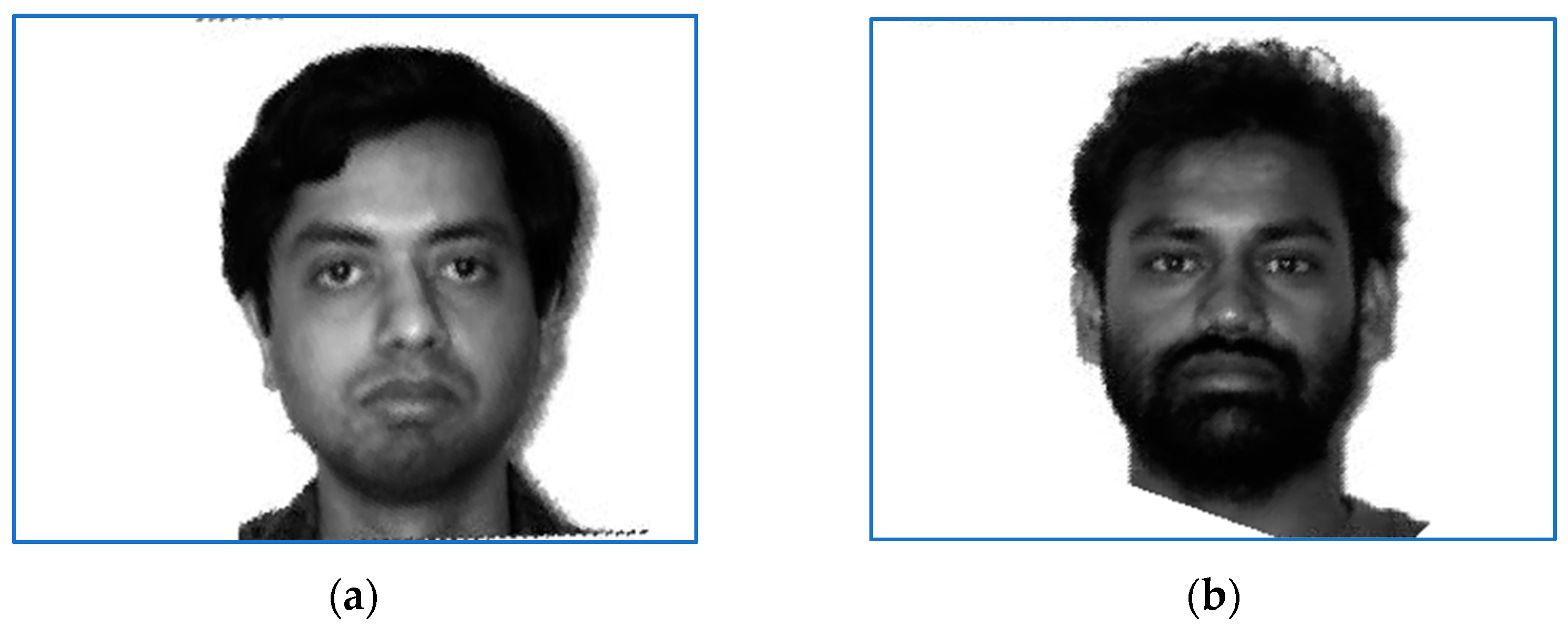
Below, we provide a summary of the registration results obtained for images belonging to the Yale Face Database [29]. The database consists of 165 monochrome face images of 15 persons, 11 samples for each. The spatial resolution for all images is 320 × 243 pixels.

Table 1. The recorded runtimes for Algorithms 1 and 2.

Picture Number	MeanRT Algorithm 2	Standard Deviation Algorithm 2	MeanRT Algorithm 1	Standard Deviation Algorithm 1
1	16.683	13.840	39.226	51.040
2	7.032	4.448	18.024	12.859
3	8.693	9.794	21.973	34.752
4	9.279	6.536	19.962	14.004
5	10.875	9.985	26.616	34.338
6	27.259	25.174	81.579	80.575
7	6.592	6.219	17.904	14.108
8	9.898	8.019	19.449	11.861
9	9.992	8.588	14.837	14.519
10	45.863	35.704	73.085	95.596
11	17.577	11.032	32.336	17.693
12	3.713	2.134	7.921	3.138
13	7.026	4.049	14.868	8.589
14	12.279	8.817	29.684	20.397
15	22.550	21.484	78.269	79.963
16	16.881	13.385	40.910	33.674
17	10.417	8.510	25.807	44.410
18	6.941	4.229	19.458	14.295
19	9.059	7.981	14.484	8.955
20	6.998	4.559	12.114	8.604
21	5.218	2.388	10.452	6.977
22	15.622	11.741	36.905	50.612
23	10.943	12.642	23.850	24.620
24	7.110	6.141	17.508	13.665
25	6.595	4.438	17.884	15.519
26	3.500	2.740	8.466	4.721
27	10.334	8.059	27.193	24.778
28	8.165	7.235	24.559	23.945
29	6.027	4.516	20.026	23.594
30	4.437	3.095	15.116	11.412
Mean value	11.452	9.249	27.015	26.774

,

Table 2. RSNR values and success rates – Algorithm 2, PAT and RS-GD.

Picture Number	MeanRSNR Algorithm 2	Standard Deviation Algorithm 2	Correct Alignment Algorithm 2	RSNR PAT	Correct Alignment PAT	RSNR RS-GD	Correct Alignment RD-GD
1	0.911	0.022	1	0.401	0	0.538	0
2	0.808	0.033	1	0.366	0	0.874	1
3	0.738	0.051	1	0.317	0	0.877	1
4	0.872	0.042	1	0.354	0	0.887	1
5	0.887	0.046	1	0.442	0	0.438	0
6	0.775	0.064	1	0.275	0	0.421	1
7	0.959	0.019	1	0.822	1	0.765	1
8	0.978	0.009	1	0.874	1	0.803	1
9	0.820	0.036	1	0.407	0	0.395	0
10	0.876	0.039	1	0.424	0	0.482	0
11	0.843	0.050	1	0.325	0	0.921	1
12	0.884	0.039	1	0.400	0	0.940	1
13	0.817	0.015	1	0.770	1	0.876	1
14	0.885	0.037	1	0.854	1	0.377	0
15	0.826	0.038	1	0.321	0	0.428	0
16	0.808	0.016	1	0.375	0	0.892	1
17	0.842	0.045	1	0.322	0	0.928	1
18	0.937	0.022	1	0.777	1	0.977	1
19	0.761	0.048	1	0.306	0	0.826	1
20	0.853	0.041	1	0.443	0	0.515	0
21	0.945	0.029	1	0.251	0	0.360	0
22	0.730	0.048	1	0.358	0	0.440	0
23	0.870	0.049	1	0.364	0	0.405	0
24	0.750	0.021	1	0.344	0	0.894	1
25	0.943	0.029	1	0.733	1	0.984	1
26	0.768	0.038	1	0.366	0	0.441	0
27	0.928	0.027	1	0.584	1	0.471	0
28	0.883	0.037	1	0.767	1	0.925	1
29	0.774	0.034	1	0.434	0	0.392	0
30	0.784	0.035	1	0.347	0	0.408	0
Mean value	0.848	0.035	1	0.471	0.267	0.663	0.533

,

Table 3. The ${\mathrm{RNMI}}^{\mathrm{S}}$ values—Algorithm 2, PAT and RS-GD.

Picture Number	${\mathbf{MeanRNMI}}^{\mathbf{S}}\mathbf{Algorithm}\mathbf{2}$	Standard Deviation Algorithm 2	${\mathbf{RNMI}}^{\mathbf{S}}\mathbf{PAT}$	${\mathbf{RNMI}}^{\mathbf{S}}$ RS-GD
1	0.830	0.032	0.317	0.437
2	0.862	0.040	0.419	1.012
3	0.802	0.038	0.362	0.997
4	0.929	0.025	0.390	1.015
5	0.923	0.031	0.426	0.443
6	0.864	0.041	0.369	0.976
7	0.873	0.042	0.580	1.025
8	0.875	0.027	0.620	1.027
9	0.853	0.035	0.453	0.504
10	0.845	0.036	0.400	0.442
11	0.866	0.041	0.379	1.025
12	0.897	0.035	0.408	1.024
13	0.903	0.021	0.835	1.009
14	0.913	0.033	0.801	0.342
15	0.881	0.030	0.340	0.458
16	0.797	0.021	0.383	1.017
17	0.866	0.035	0.393	1.018
18	0.872	0.032	0.712	1.037
19	0.876	0.032	0.357	0.994
20	0.888	0.044	0.404	0.446
21	0.872	0.022	0.356	0.364
22	0.820	0.040	0.395	0.470
23	0.871	0.050	0.421	0.465
24	0.809	0.019	0.383	1.014
25	0.904	0.039	0.616	1.040
26	0.825	0.032	0.396	0.488
27	0.876	0.031	0.522	0.427
28	0.886	0.037	0.729	1.010
29	0.859	0.034	0.486	0.424
30	0.858	0.033	0.429	0.520
Mean value	0.866	0.034	0.469	0.749

and

Table 4. The ${\mathrm{RNMI}}_{\mathsf{\alpha }}^{\mathrm{T}}$ values—Algorithm 2, PAT and RS-GD.

Picture Number	${\mathbf{MeanRNMI}}_{\mathbf{\alpha }}^{\mathbf{T}}\mathbf{Algorithm}\mathbf{2}$	Standard Deviation Algorithm 2	${\mathbf{RNMI}}_{\mathbf{\alpha }}^{\mathbf{T}}$ PAT	${\mathbf{RNMI}}_{\mathbf{\alpha }}^{\mathbf{T}}$ RS-GD
1	0.935	0.013	0.658	0.796
2	0.947	0.015	0.705	0.978
3	0.911	0.020	0.655	0.973
4	0.972	0.010	0.672	0.977
5	0.970	0.012	0.741	0.765
6	0.944	0.018	0.694	0.940
7	0.949	0.018	0.830	0.980
8	0.965	0.009	0.856	0.982
9	0.942	0.015	0.712	0.748
10	0.938	0.015	0.713	0.756
11	0.948	0.016	0.718	0.995
12	0.965	0.014	0.698	0.989
13	0.956	0.008	0.898	0.969
14	0.965	0.014	0.850	0.597
15	0.944	0.013	0.621	0.745
16	0.922	0.009	0.680	0.977
17	0.946	0.016	0.655	0.978
18	0.955	0.012	0.882	0.996
19	0.944	0.016	0.624	0.973
20	0.952	0.019	0.668	0.695
21	0.951	0.008	0.734	0.709
22	0.923	0.017	0.655	0.751
23	0.947	0.021	0.695	0.744
24	0.913	0.008	0.632	0.976
25	0.959	0.017	0.845	0.986
26	0.935	0.014	0.707	0.765
27	0.955	0.013	0.823	0.716
28	0.952	0.015	0.856	0.969
29	0.925	0.019	0.785	0.715
30	0.933	0.016	0.677	0.805
Mean value	0.945	0.014	0.731	0.865

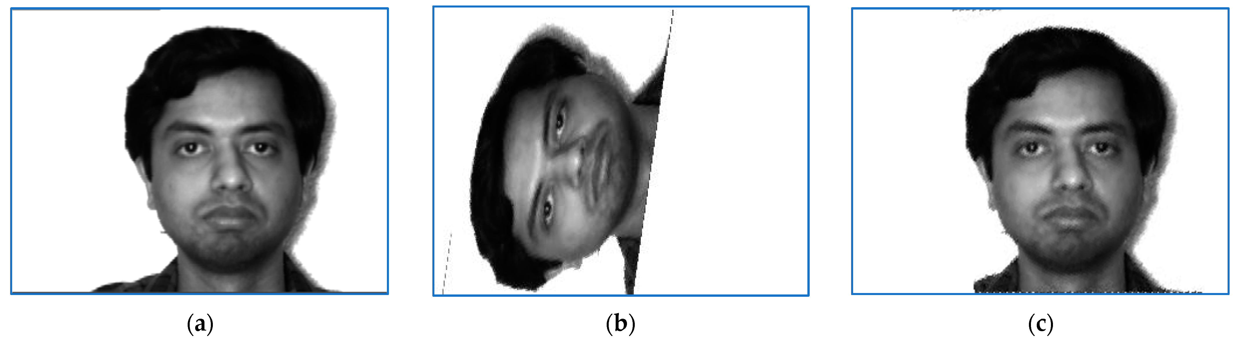
present results for 30 test images (two for each person). Figure 1, Figure 2, Figure 3, Figure 4, Figure 5, Figure 6 and Figure 7 show a selection of images for two persons that includes target, perturbed, and aligned pictures and also binarized and scaled versions used during computations.

The perturbation model is given by (11), with the parameters: $\mathsf{\theta }\in \left[-\frac{\mathsf{\pi }}{2},0\right]$, ${\mathrm{s}}_{\mathrm{x}},{\mathrm{s}}_{\mathrm{y}}\in \left[0.5,1.5\right]$, $\mathrm{a}\in \left[-20,80\right]$ and $\mathrm{b}\in \left[-40,80\right]$. The sensed images shown in Figure 1 and are perturbed by $\mathrm{p}=\left[80,40,-\frac{\mathsf{\pi }}{2.2},1.5,0.8\right]$, and $\mathrm{p}=\left[10,-10,-\frac{\mathsf{\pi }}{2.1},1.1,1.35\right]$, respectively.

The proposed alignment procedure computes an approximation of the perturbation parameter vector in the search space narrowed down by the stretching factor $\mathrm{s}1=4$, while significantly larger scaling values s2 are used to generate the initial population and it prevent becoming stuck in a local optimum. In our work, the scaling parameter $\mathrm{s}2$ was between 11 and 15.

The results of applying Algorithm 2 are summarized below. Figure 1 and Figure 2 show recorded, sensed, and registered images for two test samples, subjects 10 and 7. The corresponding numerical results are presented in rows 10 and 7 in Table 1, Table 2, Table 3 and Table 4.

Figure 3 and Figure 4 represent scaled and binarized variants of the images from Figure 1 and Figure 2, computed by Algorithm 2.

Algorithm 2 parameters were set to: ${\mathsf{\tau }}_{\mathrm{stop}}\in \left[0.5,0.6\right],$ $\mathrm{n}=20$, $\mathrm{NMAX}=250$, $\mathrm{nr}=6$, $\mathrm{ind}=4$, ${\mathsf{\beta }}_0=\mathsf{\gamma }=1, {\mathsf{\sigma }}_0=\left[12, 12, 0.3, 0.5\right]$, $\mathsf{\vartheta }={\mathsf{\vartheta }}^{\prime }=0.85$, ${\mathsf{\tau }}_{\mathrm{ES}}=20$, $\mathsf{\upsilon }=0.3$, $\mathrm{MAX}=800$, ${{\mathsf{\sigma }}^{\prime }}_0=\left[7, 7, 0.03, 0.05\right]$, ${{\mathsf{\tau }}^{\prime }}_{\mathrm{ES}}=15,$ ${\mathrm{MAX}}^{\prime }=240$, $\mathrm{it}=3$, and ${\mathrm{it}}^{\prime }=7$. Each time the algorithm gets caught by a local optimum, ${\mathrm{k}}_0=7$ new locally improved individuals and the result computed by Algorithm 1 with $\mathrm{s}2=15$ replace ${\mathrm{k}}_0+1$ individuals belonging to the current population. Note that the parameters’ values used in 2MES and FA algorithms are set in line with values widely used in various reported works [19,20,21], which constitute a de facto standard.

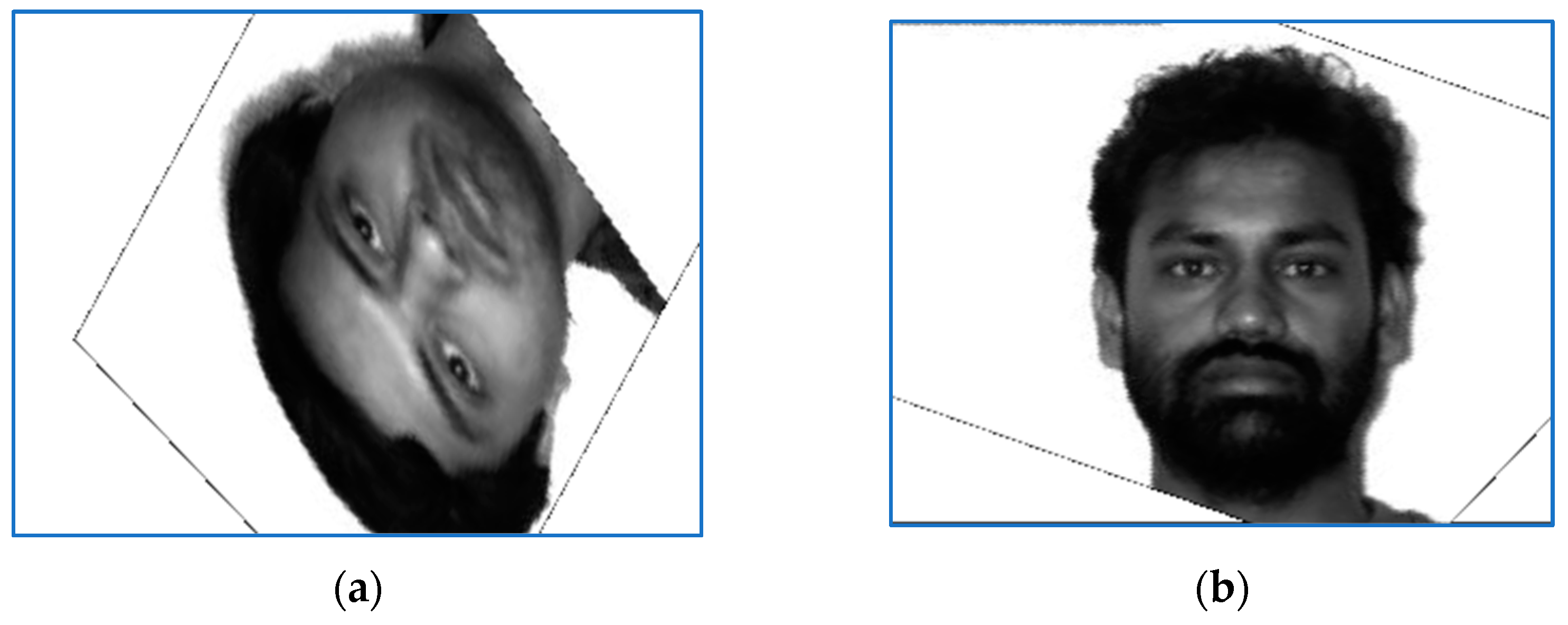
Figure 5 present the alignment results of Algorithm 2.

The proposed algorithm has yielded a perfect success rate, correctly aligning all the test image pairs. Note that Algorithm 1 correctly aligns the considered images, but the recorded runtimes are substantially larger than those obtained by the proposed method. The numeric results reported below refer to the mean value and the standard deviation of the runtimes computed for Algorithms 2 and 1, respectively. The data in Table 1 prove that Algorithm 2 is significantly faster than Algorithm 1.

The mean values and the standard deviation values computed for the accuracy measures are displayed in Table 2, Table 3 and Table 4. Note that we used $\mathsf{\alpha }=1.2$ to compute the Tsallis mutual information. The maximum value of the functions defined by (31) is 1, but due to rounding and computation errors, slightly larger values may be obtained.

Additionally, in order to derive comprehensive conclusions regarding the performances of Algorithm 2, we tested it against two classical methods for monomodal image registration, the regular step gradient descent optimization (RS-GD) based on mean squares image similarity metric (MS) [30,31], and Principal Axes Transform (PAT) [18]. RS-GD based registration adjusts the geometric transformation parameters so that the evolution of the considered metric is toward the extrema. PAT is an image registration technique based on features automatically extracted from images, where the image features are defined by the corresponding set of principal axes.

Figure 6 present the results of applying the PAT method, and Figure 7 present the results of applying the RS-GD algorithm.

The accuracy results of all tested methods are reported in Table 2, Table 3 and Table 4. The mean and standard deviation values of RSNR correspond to Algorithm 2 and RSNR values recorded for PAT and RS-GD are provided in Table 2. In addition, Table 2 show the success ratios of Algorithm 2 and whether classical methods managed to correctly align the tested pairs of images. Note that, in the case of severely perturbed sensed images, both classical methods may misregister the inputs. The resulted accuracy rate of PAT is only 26.7%, while for RS-GD, it is 53.3%. Algorithm 2 had a 100% accuracy, correctly registering all tested images in all runs.

The mean and standard deviation values of ${\mathrm{RNMI}}^{\mathrm{S}}$ and ${\mathrm{RNMI}}_{\mathsf{\alpha }}^{\mathrm{T}}$ computed in the case of Algorithm 2 are displayed in Table 3 and Table 4, respectively. The tables also present the values of ${\mathrm{RNMI}}^{\mathrm{S}}$and ${\mathrm{RNMI}}_{\mathsf{\alpha }}^{\mathrm{T}}$ corresponding to PAT and RS-GD methods.

The numerical results indicate that Algorithm 2 produces more accurate results than PAT and RS-GD in the light of all informational and quantitative indicators used. In addition, the new method is considerably faster than the method reported in [1].

6. Conclusions

The aim of the paper was to propose a new comprehensive multi-scale method that extends the approach reported in [1] to obtain accurate and efficient registration algorithms. The input images were pre-processed by a noise-insensitive edge detector to obtain binarized versions, i.e., the sets containing contour pixels. Isotropic scaling transformations were used to compute multi-scale representations of the binarized inputs. The registration was then carried out in different reduced representations to obtain promising initial solutions and to identify search directions leading to the global optimum. The process combined bio-inspired and evolutionary computation techniques with clustered search and implemented a procedure specially tailored to address the premature convergence issue.

A long series of tests involving monochrome images were conducted to ascertain meaningful conclusions regarding the registration capabilities of the proposed method. The experiments involved accuracy and efficiency measures, expressed in terms of SNR, Shannon mutual information, Tsallis entropy, and runtime. We compared Algorithm 2 against the basic method introduced in [1] and two of the most commonly used alignment procedures for monomodal images, namely the regular step gradient descent optimization based on MS image similarity metric and PAT registration. In terms of accuracy, Algorithm 2 is similar to Algorithm 1, with a success rate of 100%, which means that it has always managed to correctly align the input images. In contrast, both RS-GD and registration and PAT alignment failed to solve the problem of severely perturbed sensed images, their corresponding success rate being far less than 100%. In terms of efficiency, there were significant improvements over Algorithm 1, with the proposed method being at least two times faster.

The experimentally established results validate the proposed method and open the path for further developments and extensions to more complex transformations. In addition, metaheuristics involving other promising bio-inspired techniques, such as the flower pollination algorithm, cuckoo search, and bat algorithm, will be considered for the population-based optimization component. In addition, an experimental study on the influence of parameter values on the performance of the proposed method is in progress.