An Application-Oriented Method Based on Cooperative Map Matching for Improving Vehicular Positioning Accuracy

Abstract

Accurate vehicular positioning is important for intelligent and connected vehicles (ICVs). However, in urban canyons, vehicles that rely solely on global navigation satellite system (GNSS) are susceptible to factors such as signal blocking and multi-path, reducing the positioning performance. In this paper, an application-oriented cooperative map matching (CMM) method is proposed, and a low-cost Global Positioning System (GPS)/BeiDou navigation satellite system (BDS) integrated positioning system is designed. The road constraints of a real traffic environment, which simplifies the computational complexity and facilitates practical applications, are modeled. The positioning system is designed to collect and store the positioning data for experimental analysis. Static and dynamic experiments are conducted to verify the effectiveness of the CMM method. From the experimental results, the mean absolute error (MAE) and root mean square error (RMSE) of the positioning with CMM correction in the static experiment are reduced by 9.0% and 4.9%, respectively. In the dynamic experiment, compared with the original positioning error, the MAE is reduced by 44.2% while the RMSE is reduced by 24.3%. The results show that the proposed method can improve vehicular positioning accuracy effectively in both static and dynamic environments.

1. Introduction

Over the past years, intelligent transportation systems have been developed rapidly. As an essential component of intelligent transportation systems, the navigation system can provide location information for vehicles. A GNSS determines its position by calculating pseudoranges of multiple satellites [1]. Generally, the errors of pseudoranges are divided into common error and non-common error. Common error is mainly caused by satellite clock error, ionospheric error, ephemeris error, and tropospheric error [2]. Non-common error includes receiver noise, receiver clock error, and multipath error [3]. The high accuracy of location is critical for intelligent connected vehicles [4]. However, low-cost satellite receivers deployed in vehicles suffer from the problems of low positioning accuracy, insufficient reliability, and frequent signal loss. For example, the nominal accuracy of Global Positioning System (GPS) is about 15 to 20 meters [5], which might not be sufficient for the applications in the field of safe driving, such as lane-level positioning.

Many methods can be used to improve accuracy for ego-localization. A common approach is to fuse the GNSS data with other embedded information sources such as dead reckoning (DR) sensors, inertial navigation system (INS), video cameras, and radar [6,7,8,9]. Data fusion algorithms (e.g., classical Kalman filter and particle filter [10]) are used to process the fused information for obtaining more accurate localization positions. Differential GNSS (DGNSS) is an enhancement to GNSS that can improve the positioning accuracy to sub-meter level [11]. In DGNSS, the position information received by the base station receiver is corrected with the precise position of the fixed base station, and then the correction values are broadcast to nearby users for improving the positioning accuracy. Then centimeter-level accuracy or decimeter-level accuracy is achieved by the real-time kinematic (RTK) in an outdoor environment [12]. Precision point positioning (PPP) can reach a level of positioning accuracy at the decimetre level; the performance level of PPP is usually close to the level that can be achieved by the differential method [13,14]. However, these methods rely on expensive infrastructure, and there is large positioning error in areas such as urban and canyons.

With the emergence of vehicular ad hoc networks (VANETS), and the development of dedicated short range communication (DSRC) technologies, cooperative positioning (CP) provides an alternative for improving positioning performance [15,16]. However, there are data security and delay problems when vehicles are sharing information. Song et al. [17] proposed a novel framework blockchain-based ICVs that improves and ensures data security. Ansari et al. [18] proposed a relative position prediction mechanism to cover the problem that the data contained in the DRSC messages may soon become outdated. Rabiee et al. [19] proposed a new particle-filter-based information fusion algorithm to achieve lane-level tracking accuracy in GNSS-denied environments, which achieves a lane-level positioning RMES of no more than 1.5 m. However, some additional sensors such as radar and inertial measurement unit (IMU), could result in the problems of increasing equipment cost and algorithm complexity. Amini et al. [20] proposed a comprehensive positioning algorithm that utilizes all data from different sources, which significantly improves vehicle positioning accuracy under the condition of weak GPS signals. Mahmoud et al. [21] presented a new unified cooperative localization solution that improves localization accuracy and usability in urban canyons. However, a disadvantage of INS is that the accumulated error will increase over time [22]. Liu et al. [23] presented a distributed location estimation algorithm based on vehicle-to-vehicle distance detection to improve the accuracy of vehicle localization. This method only relies on the pseudoranges of GPS and the detected inter-vehicle distance without any reference point for positioning error correction. Nonetheless, this data-sharing-based approach may cause data incest, which often leads to over-convergence issues. Xu et al. [24] proposed a Gaussian condensation filter algorithm based on error-ellipse resampling, which can effectively eliminate accumulated error and outperform particle filtering. Liu et al. [25] presented a novel robust cubature Kalman filter to improve data fusion performance in uncertain sensor observation environments.

Map matching is a method of cooperative positioning, which could correct the position deviation from the road by combining the measured GPS position with the accurate digital map. Based on geometric analysis and topological analysis, the current map matching methods are mainly divided into three categories: geometric, topological, and advanced. With the development of high-precision digital maps, cooperative positioning algorithms based on map matching have been widely studied [26,27,28,29]. In urban environments, these studies are devoted to improving lane-level localization accuracy of visual map matching. Although these studies have obtained relatively satisfactory results, visual equipment do not work well in certain weather conditions. Thus, it is necessary to add other sensor equipment, but it increases the cost of positioning. Additionally, these methods also incorporate other algorithms (e.g., supervised neural network and robust lane marking detection), which increase the computational complexity. Rohani et al. [30] presented a novel CMM approach to improve vehicular positioning, which is based on the cooperation of vehicles by communicating their positioning information for improving vehicular positioning. However, the road constraints of real roads are not easily described by mathematical analysis. Shen et al. [31] presented a particle-based CMM algorithm to eliminate the common biases and reduce the positioning error, but it may lead to a lack of particle diversity.

The cooperative positioning algorithms mentioned above could improve the positioning accuracy effectively. However, it is still challenging to achieve a balance between the positioning accuracy, computational complexity, and receiver cost. In this paper, a simplified CMM method with road constraint model is conducted, and a low-cost positioning system is designed to verify the effectiveness. The main contributions can be summarized as follows:

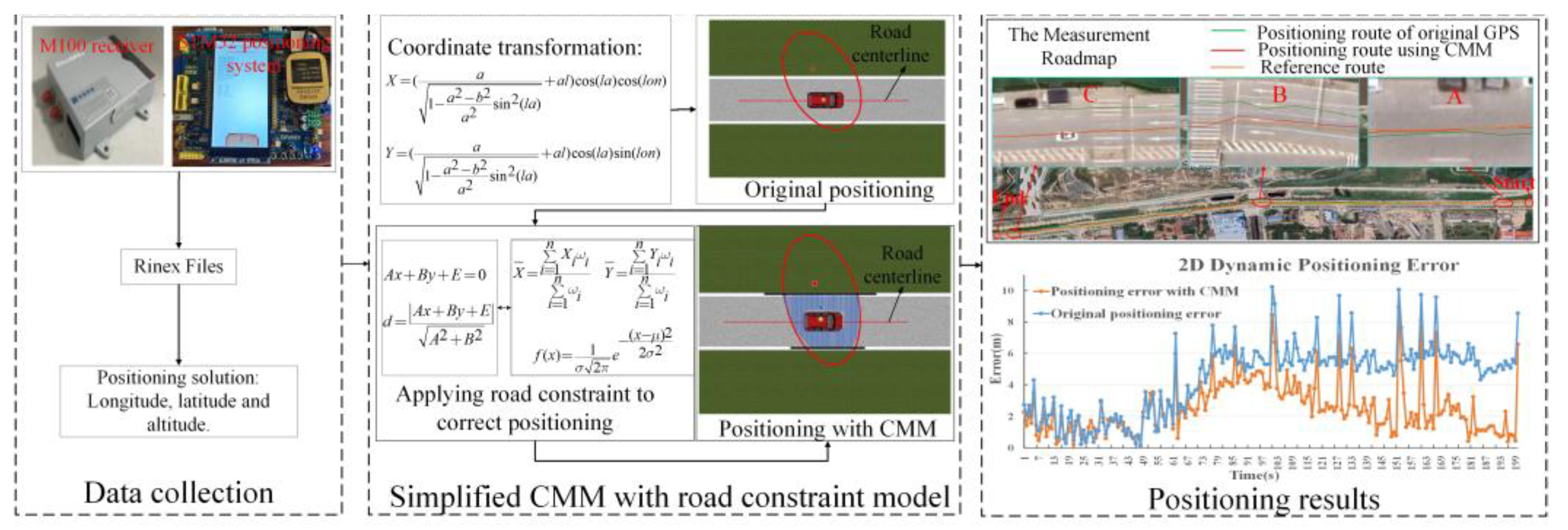
• A CMM method is designed to optimize the positioning effect combined with high-precision digital map. The road coordinate system is established according to the map, and the road constraints are modeled, which realizes the analysis and description of the position constraints, simplifies the calculation complexity, and facilitates practical application.
• A low-cost GPS/BDS integrated positioning system, which can realize real-time vehicular positioning and store the positioning data, is designed and implemented.
• The vehicular positioning data are collected in the real traffic scene, and the effectiveness of the proposed CMM method is verified on the collected dataset.

The rest of this paper is organized as follows. In Section 2, the CMM and the modeling process of road constraints are detailed. Section 3 presents and analyzes the static and dynamic experimental results. Finally, conclusions are provided in Section 4.

2. Cooperative Map Matching Method

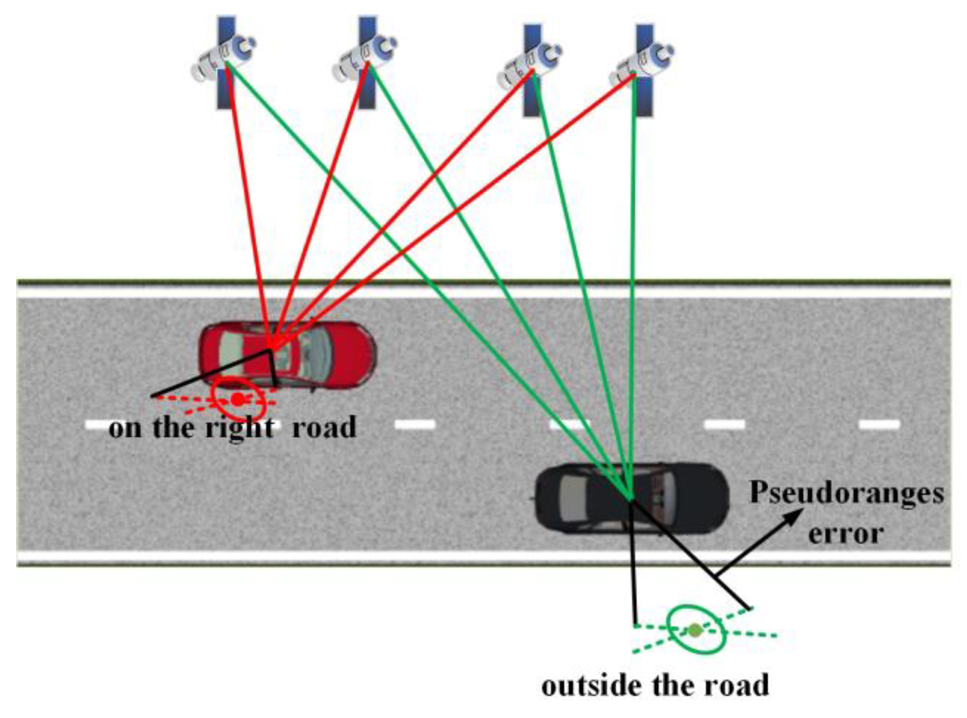
2.1. Method Description

Biased localization can be caused by the influence of pseudoranges error. As shown in Figure 1, due to the pseudoranges error, the position of the black vehicle is not located in its lane, and the red vehicle is in its lane but not in an exact location.

As mentioned above, both the common and non-common error, can result in the biased localization. The key idea of the CMM method is to use the known precise position information of the high-precision map as a constraint to effectively reduce the pseudoranges error, so that the biased localization can be corrected for a more precise position. The overall process of CMM correction positioning is shown in Figure 2.

2.2. Pseudoranges Calculation

Positioning accuracy is largely determined by the pseudoranges measurement. The formula of pseudoranges can be calculated as

$${\rho }_j^{(i)}=D_j^{(i)}+c\delta t^{(i)}+{\zeta }_j^{(i)}+{\eta }^{(i)}$$

(1)

where ${\rho }_j^{(i)}$ is the measured pseudoranges from $j\mathrm{th}$ satellite to $i\mathrm{th}$ GPS receiver, $D_j^{(i)}$ is the true distance from the $j\mathrm{th}$ satellite to the $i\mathrm{th}$ GPS receiver, $c$ is the speed of light, $\delta t^{(i)}$ is the clock error between receiver and satellite, ${\zeta }_j^{(i)}$ is the common error, and ${\eta }^{(i)}$ is the un-common error.

The estimated position $X^{(i)}=[x^{\left(i\right)},y^{\left(i\right)},z^{\left(i\right)}]$ of $i\mathrm{th}$ vehicle can be obtained from the GPS receiver. Position of the $j\mathrm{th}$ satellite is $X^{\left(j\right)}=[x^{(j)},y^{(j)},z^{(j)}]$, and geometric distance from the $i\mathrm{th}$ vehicle to the $j\mathrm{th}$ satellite is

$$D_j^{(i)}=\sqrt{{(x^{(j)}-x^{(i)})}^2+{(y^{(j)}-y^{(i)})}^2+{(z^{(j)}-z^{(i)})}^2}$$

(2)

With the utilization of CMM, the estimated position of the $i\mathrm{th}$ vehicle can be calculate as $\widetilde{X^{(i)}}=[\widetilde{x^{(i)}},\widetilde{y^{(i)}},\widetilde{z^{(i)}}]$, and the geometric distance between $i\mathrm{th}$ vehicle and $j\mathrm{th}$ satellite is

$${\tilde{D}}_j^{(i)}=\sqrt{{(x^{(j)}-\widetilde{x^{(i)}})}^2+{(y^{(j)}-\widetilde{y^{(i)}})}^2+{(z^{(j)}-\widetilde{z^{(i)}})}^2}$$

(3)

In the CMM, although the non-common error of pseudoranges for adjacent vehicles is approximated, influence of the error must be considered. If the error is ignored, it may cause over convergence to a non-true position, which would seriously affect the positioning accuracy. However, the non-common error is independent for each vehicle, and the error varies rapidly. Therefore, in order to accurately analyze the error, we use the zero-mean Gaussian distribution to model the non-common error as follows:

$${\eta }^{(i)}~N(0,{{\sigma }_{\eta }}^2)$$

(4)

Since the map is a static image, there are some defects where it cannot fully reflect the dynamic world. It is also necessary that the error effect caused by map defects should be considered in CMM method. Similarly, we consider simulating this error ${\eta }_{map}$ with a Gaussian distribution as follows:

$${\eta }_{map}~N(0,{{\sigma }_{map}}^2)$$

(5)

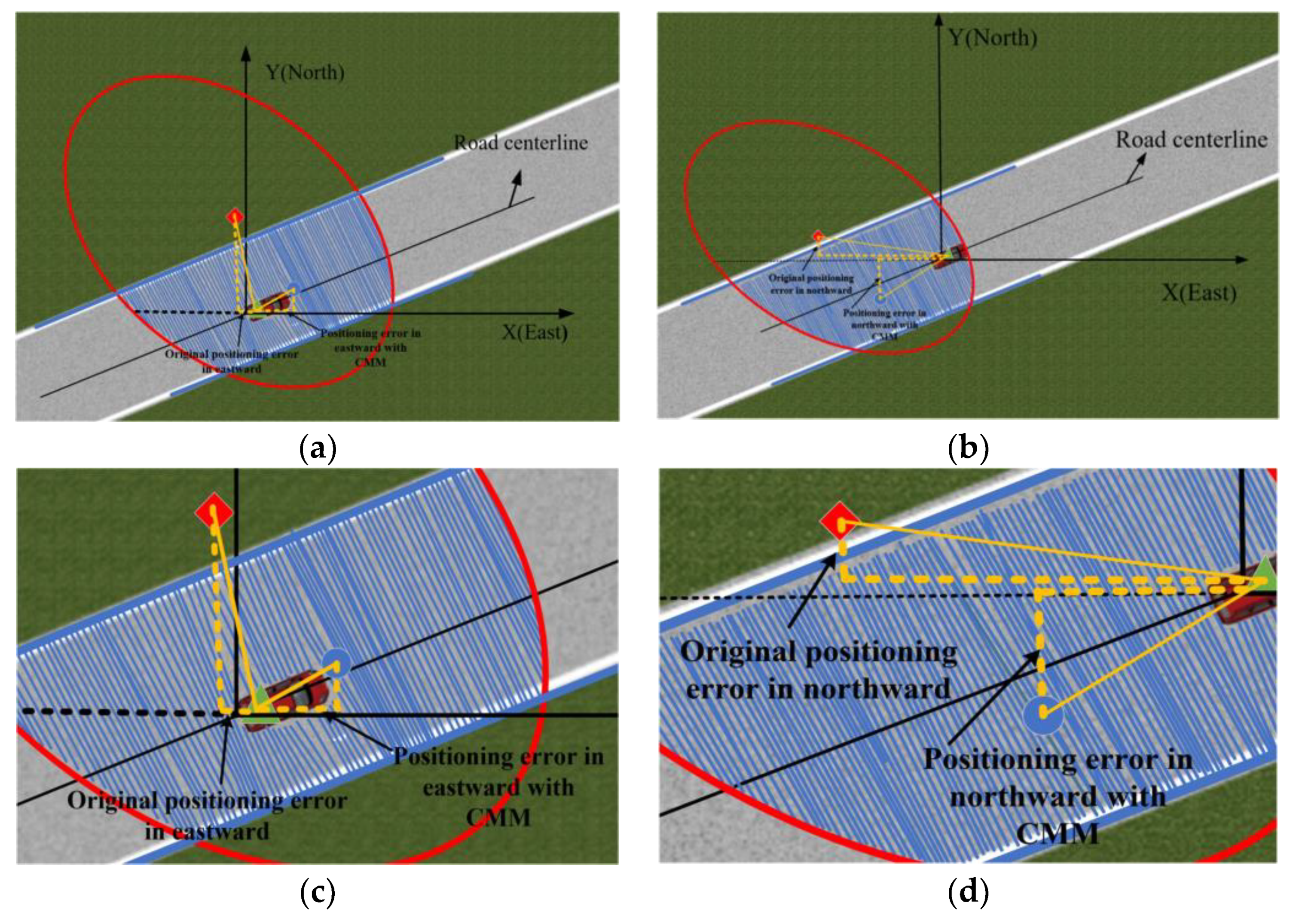
2.3. Simplified CMM with Road Constraint Model

In order to improve the positioning accuracy, an improved CMM method that applies map road constraints is proposed to improve the positioning accuracy. A receiver is fixed on the vehicle to obtain the initial measurement position. The received data from GPS are WGS-84 coordinate data which are expressed in latitude and longitude. In general, it is usually used to adopt two-dimensional plane Cartesian coordinate data. Therefore, it is necessary to convert the latitude and longitude data into plane coordinates. To obtain the plane coordinate data, we adopt the Gauss-Kruger projection method. The plane coordinate data are obtained by projecting the China Geodetic Coordinate System 2000 (CGCS2000) reference system.

$$X=(\frac{a}{\sqrt{1-\frac{a^2-b^2}{a^2}{\sin }^2(la)}}+al)\cos (la)\cos (lon)$$

(6)

$$Y=(\frac{a}{\sqrt{1-\frac{a^2-b^2}{a^2}{\sin }^2(la)}}+al)\cos (la)\sin (lon)$$

(7)

where $a$ is the major semi-axis of the ellipsoid, $b$ is the minor semi-axis of the ellipsoid, $la$ is latitude, $lon$ is longitude, and $al$ is altitude. In CGCS2000, $a$ is usually equals 6,378,137 m, and $b$ equals 6,356,752.31414 m. $X$ is the longitude in two-dimensional plane Cartesian coordinates, and $Y$ is the latitude in two-dimensional plane Cartesian coordinates.

The straight line of the lane center can be obtained from the digital map:

$$Ax+By+E=0$$

(8)

where $A$ and $B$ are the coefficients of the variables of the straight line, and $E$ is the intercept of the equation. Distance from the plane coordinate position of the vehicle to the lane center equation can be expressed as

$$d=\frac{\left|Ax+By+E\right|}{\sqrt{A^2+B^2}}$$

(9)

When the distance is greater than half the lane width, the vehicle position is not within the lane. We implement the CMM through particle filtering. Firstly, according to the GPS measurement positioning, $M$ particles can be started. Then, we reset the weight of the particle on the basis of distance $d$ from the particle to the lane center. When the particle is not in the lane, the weight is set to 0, and remaining particles $n$ are reserved. Finally, the weighted average of the remaining particles is viewed as the estimated position.

$$\stackrel{-}{X}=\frac{{\displaystyle \sum _{k=1}^n{X}_k{\omega }_{xk}}}{{\displaystyle \sum _{k=1}^n{\omega }_{xk}}} ,\stackrel{-}{Y}=\frac{{\displaystyle \sum _{k=1}^n{Y}_k{\omega }_{yk}}}{{\displaystyle \sum _{k=1}^n{\omega }_{yk}}}$$

(10)

where $\stackrel{-}{X}$ and $\stackrel{-}{Y}$ are the weighted average of dataset $X_k$ and $Y_k$, respectively. ${\omega }_{xk}$ and ${\omega }_{yk}$ are the weight of $X_k$ and $Y_k$, respectively. The $M$ particles are initialized with a Gaussian distribution, where the standard deviation is

$$\sigma ={\sigma }_{\eta }+{\sigma }_{map}$$

(11)

Moreover, the value of the random variable μ is the plane coordinates of the actual measurement position. During the data processing, the standard deviation σ is the distance between the actual measurement position and precise position at the same timestamp. The weight corresponding to each initial particle is

$${\omega }_k=\frac{1}{\sigma \sqrt{2\pi }}{e}^{-\frac{{(x-\mu )}^2}{2{\sigma }^2}}$$

(12)

The principle of the road constraints model is shown in Figure 3, where the red ellipse is the uncertainty error of GPS, the red square is the measured position, the green triangle is the real position of vehicle, the black straight line represents the line centerline, the blue area is the GPS error range after applying the map road constraints, and the blue dot is the corrected position.

Figure 3 reveals the principle of the CMM method applying the road constraint model. When applying the road constraint model for map matching, the road constraints are mainly used to correct the positioning error in the direction perpendicular to the line, and there are no constraints in the direction parallel to the line. Therefore, the proposed CMM method may not improve the error effectively or even increase the error in the sub-direction, but there is an effective improvement in the overall error. Figure 3a, b, respectively, present the effect of the CMM method applying the road constraint model in different sub-directions.

3. Experimental Results and Discussion

3.1. Experimental Environment

In this section, in order to verify the application-oriented effectiveness of the proposed method, a low-cost positioning system is designed to collect positioning data.

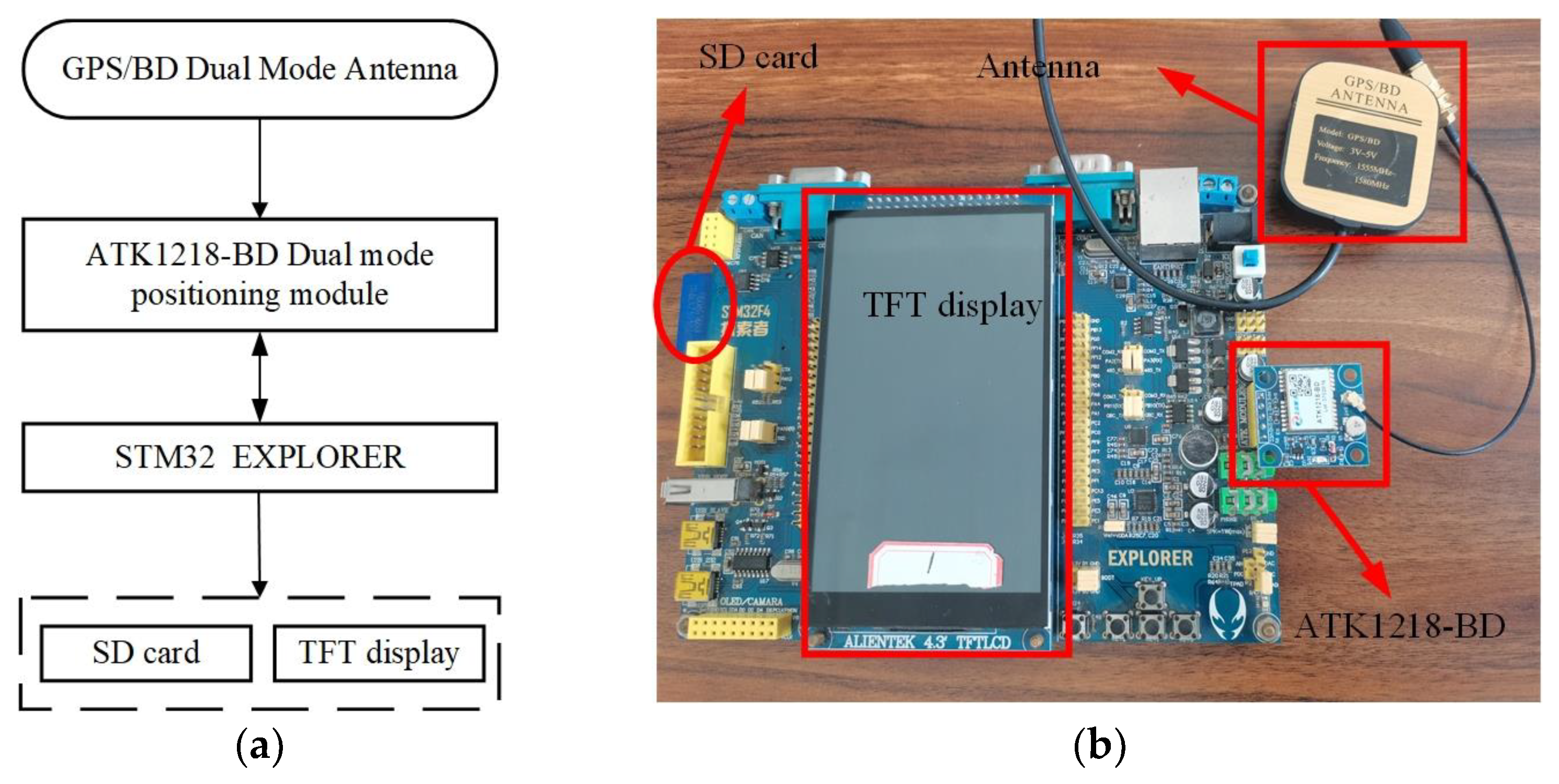
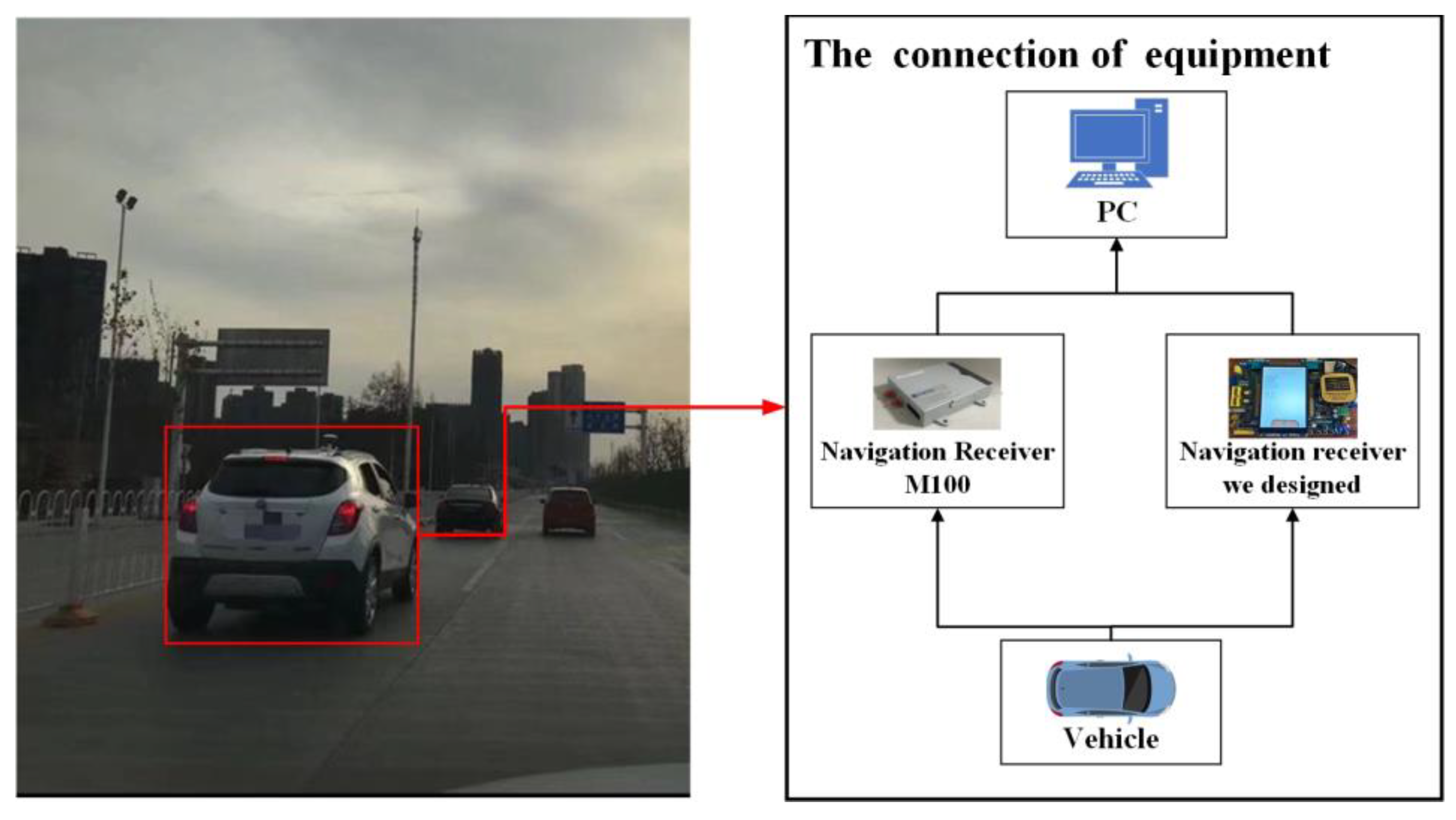
3.1.1. Positioning System Hardware Design

The hardware of the designed positioning system is mainly composed of a main controller, a secure digital (SD) card, and a positioning module, as shown in Figure 4.

In the designed system, STM32 is used as the main controller to control the calculation, storage, and display of positioning data, where the storage capacity of the SD card is 8 gigabyte. The low-cost ATK-1218-BD/GPS module is used as the positioning module. The parameters of the ATK-1218-BD/GPS module are shown in

Table 1. Parameters of ATK-1218-BD/GPS.

Item	Parameters
Positioning chip	S1216
Serial port baud rate	4800–230,400 bps
Positioning accuracy	3 m (root mean square/RMS)
Letter of agreement	NMEA-0183
Data update rate	1/2/4/5/8/10/20 Hz
Cold start time	30 s

.

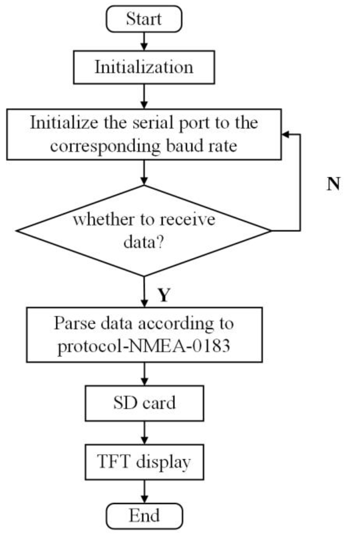
3.1.2. Positioning System Software Design

The software of the designed system analyzes the positioning data of the ATK1218-BD/GPS through the STM32 master controller, saves these data to SD card, and displays real-time positioning information through the thin film transistor (TFT) display. The algorithm process of the software is provided in Figure 5.

The received data are parsed through the national marine electronics association (NMEA) 0183 protocol. NMEA-0183 is a protocol that starts with $GPGSV and has a fixed output format to obtain latitude and longitude, speed, number of satellites, and time information. The ublox protocol realizes the setting of configuration information storage, output information, and serial port baud rate information. After receiving the GPS module data, the system analyzes, stores, and displays the GPS positioning data.

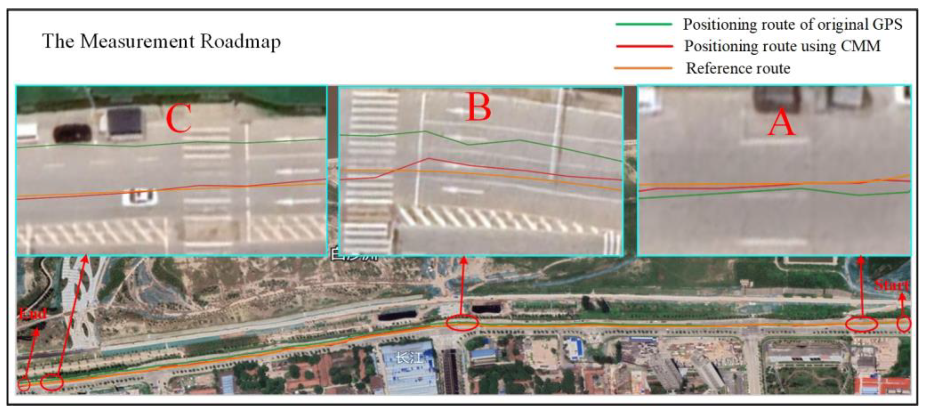
3.1.3. Test Environment

Based on the above theoretical analysis, we designed and performed a real experiment. The experimental equipment included the positioning system designed in the previous section, a Sinan M100 receiver and a computer. The GNSS antenna was mounted on top of the vehicle. The data collected by the positioning system were stored in the SD card and the data collected by the M100 receiver is stored in the computer. The M100 receiver can reach a centimeter-level accuracy in RTK positioning. Its performance parameters are shown in

Table 2. Parameters of M100 receiver.

Item	Parameters
RTK accuracy (RMS)	Horizontal: ± (10 + 1 × 10 − 6 × D) mm Vertical: ± (20 + 1 × 10 − 6 × D) mm
RTD accuracy (RMS)	Horizontal: ± 0.25 m (1 σ) Vertical: ±0.25 m (1 σ)
Single point positioning accuracy	Single frequency: H ≤ 3 m, V ≤ 5 m (1 σ, PDOP ≤ 4) Dual frequency: H ≤ 1.5 m, V ≤ 3 m (1 σ, PDOP ≤ 4)
First positioning time	Cold start < 50 s; Warm start < 45 s; Hot start < 15 s
RTK initialization time	<10 s
Signal reacquisition	<1.5 s (fast); <3.0 s (normal)
Initial confidence	>99.99%
Data update rate	1/2/5/10/20/50 Hz
Operating temperature	−40 °C~+75 °C

. Figure 6 is the connection of the test equipment.

The experiment was conducted on an open urban road along the Yangtze river in Wuhan, China. The positioning result of the low-cost positioning system was used as the information for map matching, and the positioning result of the Sinan navigation receiver M100 was used as the reference value of the real location.

The raw data were collected in both the static and dynamic environments. In the dynamic experiment, the vehicle with experimental test equipment moved at a speed range of 10~30 km/h, and the sampling interval was 1 s. The circular probability error (CEP) of the low-cost positioning system was 2.5 m. The horizontal accuracy of the M100 receiver was ±(8 + 1 × 10 − 6 × D) mm and the vertical accuracy was ±(8 + 1 × 10 − 6 × D) mm, where $D$ is the length of the baseline.

Table 3. The comparison of key parameters for ATK-1218 -BD/GPS and M100.

	Positioning Chip	Positioning Method	Positioning Accuracy (RMS)	Price
Design system (ATK-1218-BD/GPS)	S1216	Single point positioning	3 m	RMB_108
Sinan M100	ASIC	RTK	decimeter-level ± (10 + 1 × 10 − 6×D) mm	RMB_7080

provides information about key performance parameters of the design positioning system and the M100. The positioning method of the designed system is single point positioning, while that of M 100 is RTK. The price of the positioning system we designed is only 1.5% of the M100. Although the positioning accuracy is lower than that of the M100, it can satisfy the positioning requirements of many scenarios.

3.2. Experimental Results and Analysis

3.2.1. Evaluation Indicators

In the analysis of positioning results, mean absolute error (MAE) and root mean square error (RMSE) were used to evaluate the effectiveness of the CMM, which can be calculated as follows:

$$MAE=\frac{1}{W}{\displaystyle \sum _{W=1}^W\left|{\hat{U}}_W-U_W\right|}$$

(13)

$$RMSE=\sqrt{\frac{1}{W}{\displaystyle \sum _{W=1}^W{({\hat{U}}_W-U_W)}^2}}$$

(14)

where $U_W$ is positioning error value, ${\hat{U}}_W$ is the mean of $U_W$ and $W$ is the number of $U_W$.

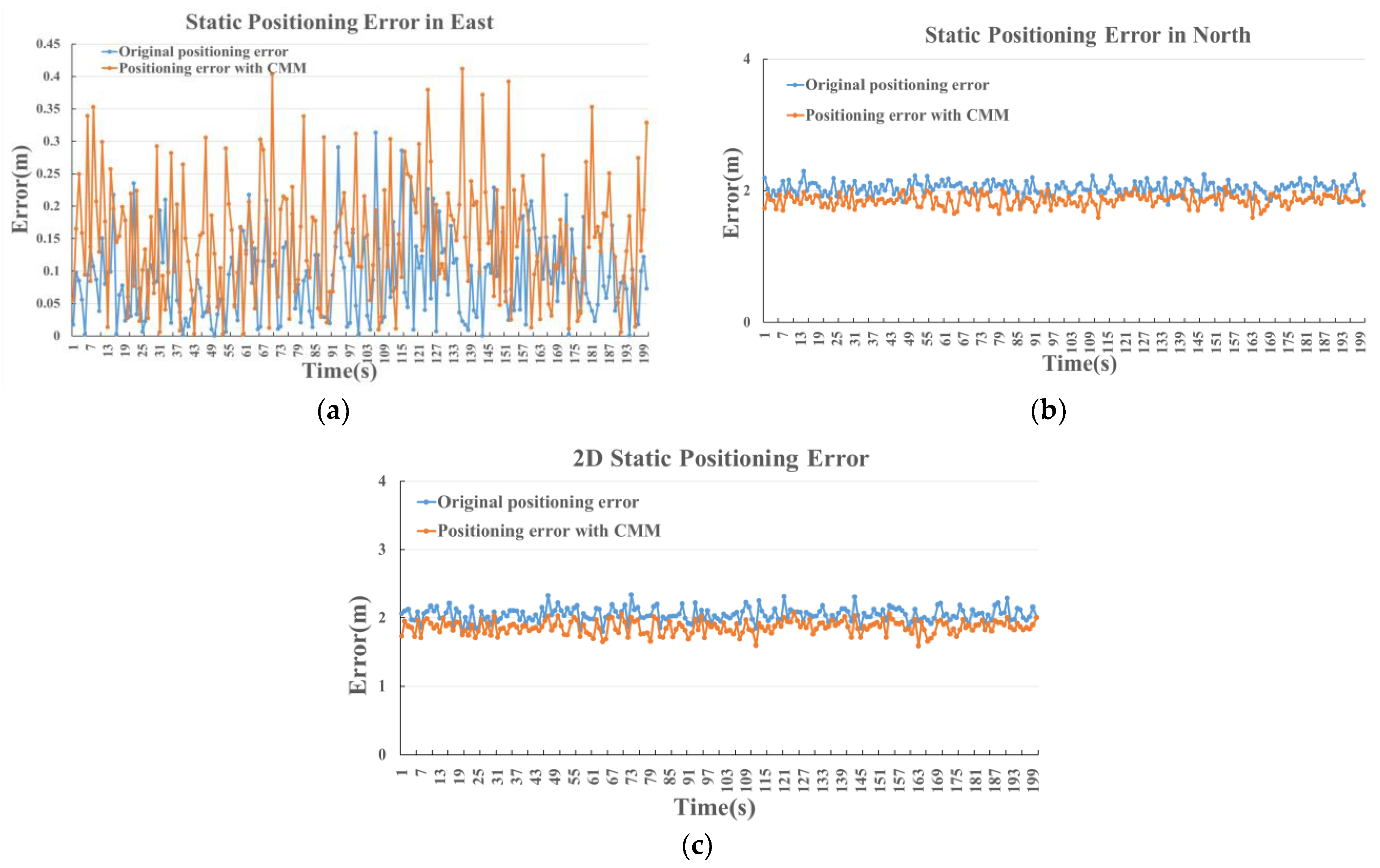
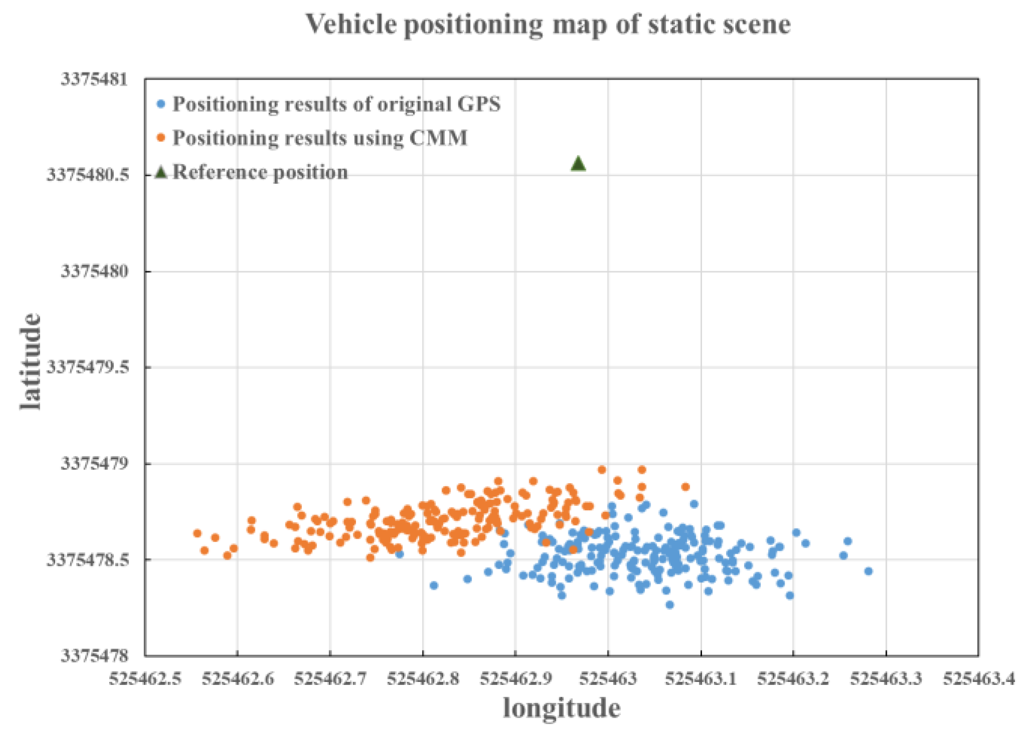
3.2.2. Static Experiment

The CMM was executed through the static positioning data collected by the low-cost positioning system. The experimental results are shown in Figure 7 and Figure 8, and the MAE and RMSE are calculated in

Table 4. The MAE and RMSE of static positioning experimental results.

	MAE (m)			RMSE (m)
	East	North	2D	East	North	2D
Original positioning	0.089	2.033	2.048	0.064	0.099	0.101
Positioning with CMM	0.151	1.854	1.863	0.091	0.092	0.096

.

From the experimental results, the MAE of 2D static positioning error is 2.048 m, which is reduced to 1.863 m through CMM correcting. As shown in Figure 7c, throughout the static experiment, the 2D positioning error with CMM correction is stable at around 1.86 m. Moreover, compared with the original 2D positioning, the overall RMSE is reduced by 4.9%. It can be found from Figure 7b that there is a significant reduction in northward error. The MAE of northward positioning is 2.033 m, which is reduced to 1.854 m. As shown in Figure 7a, the MAE is increased from 0.089 m to 0.151 m in eastward error. Figure 8 shows the positioning results of the static experiment, which is consistent with the analysis in Figure 3a.

The performance of the CMM method is further evaluated by cumulative distribution function (CDF) and probability density function (PDF) of the positioning error. CDF describes the probability that a random variable $X$ falls within a certain range, while PDF describes the probability that the random error output value is near a certain point [32]. The CDF and PDF of static experimental results are shown in Figure 9.

It can be found from the CDF that the error corresponding to the confidence level of 95% is reduced from 2.3 m to 2 m. As can be seen from the PDF, the original static positioning error is mainly distributed in the range of 1.8–2.3 m, and most of the position errors with CMM correction are reduced to the range of 1.6–2 m.

The experimental results indicate that the CMM can effectively improve the positioning accuracy in the static environment.

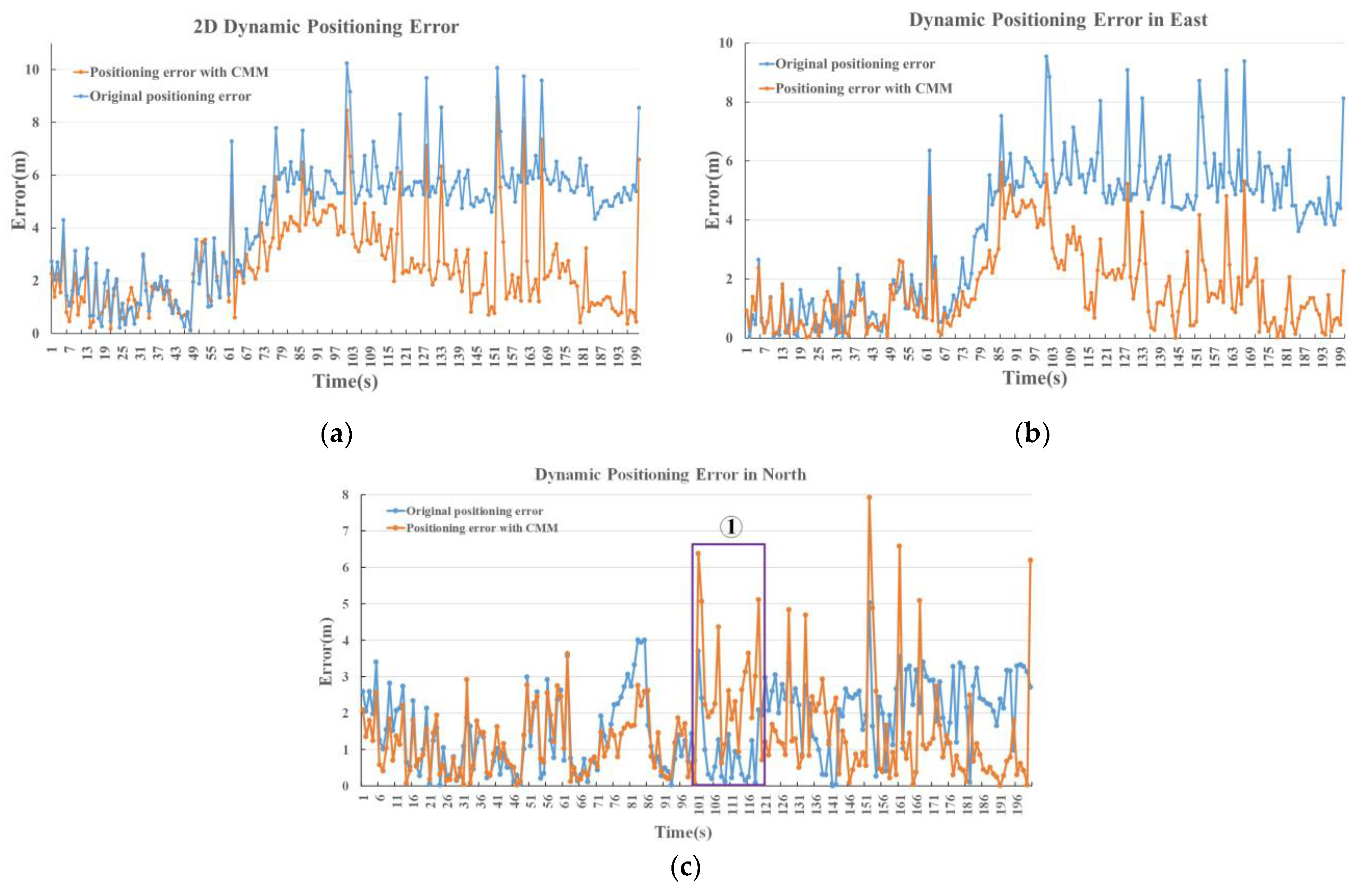
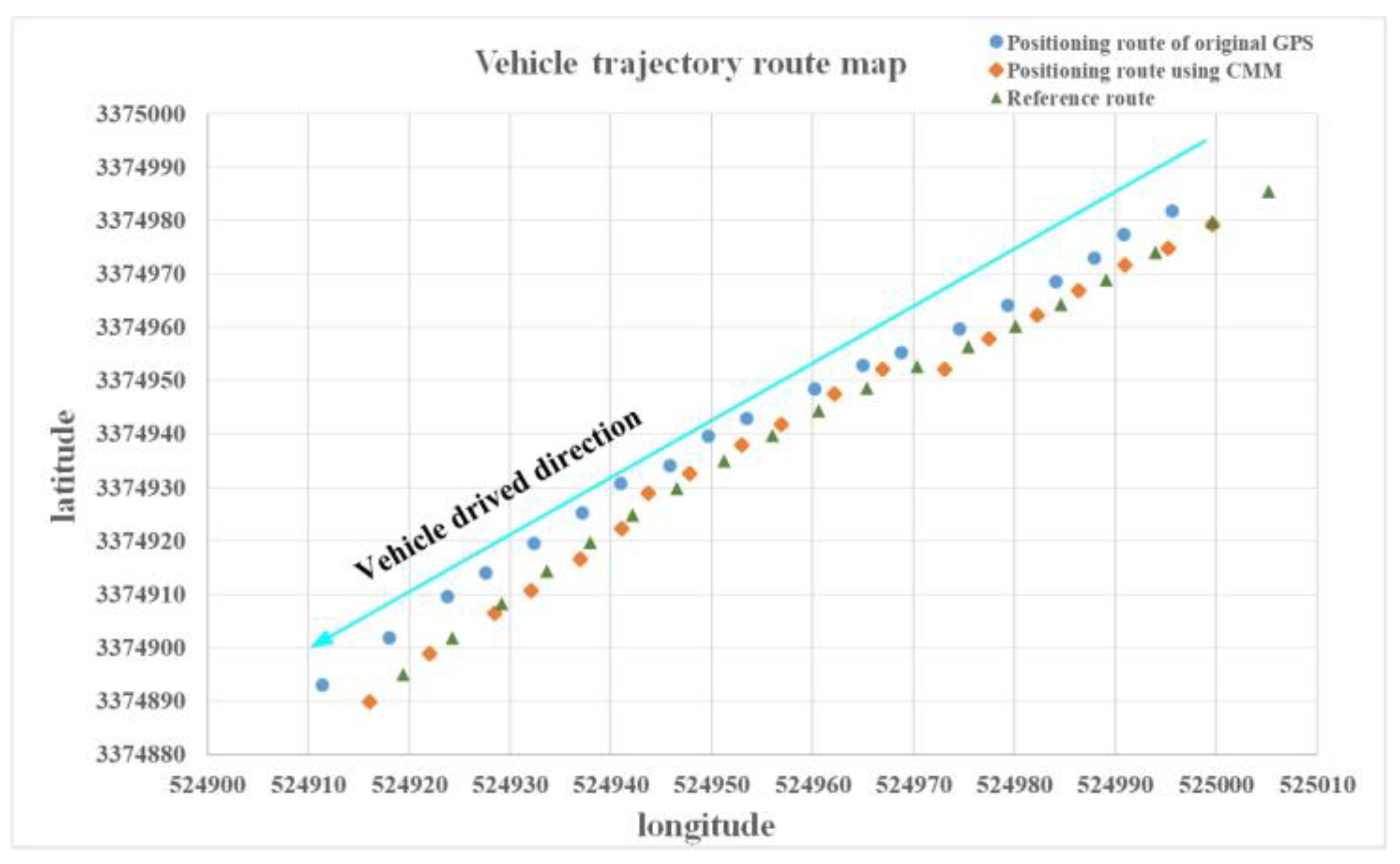
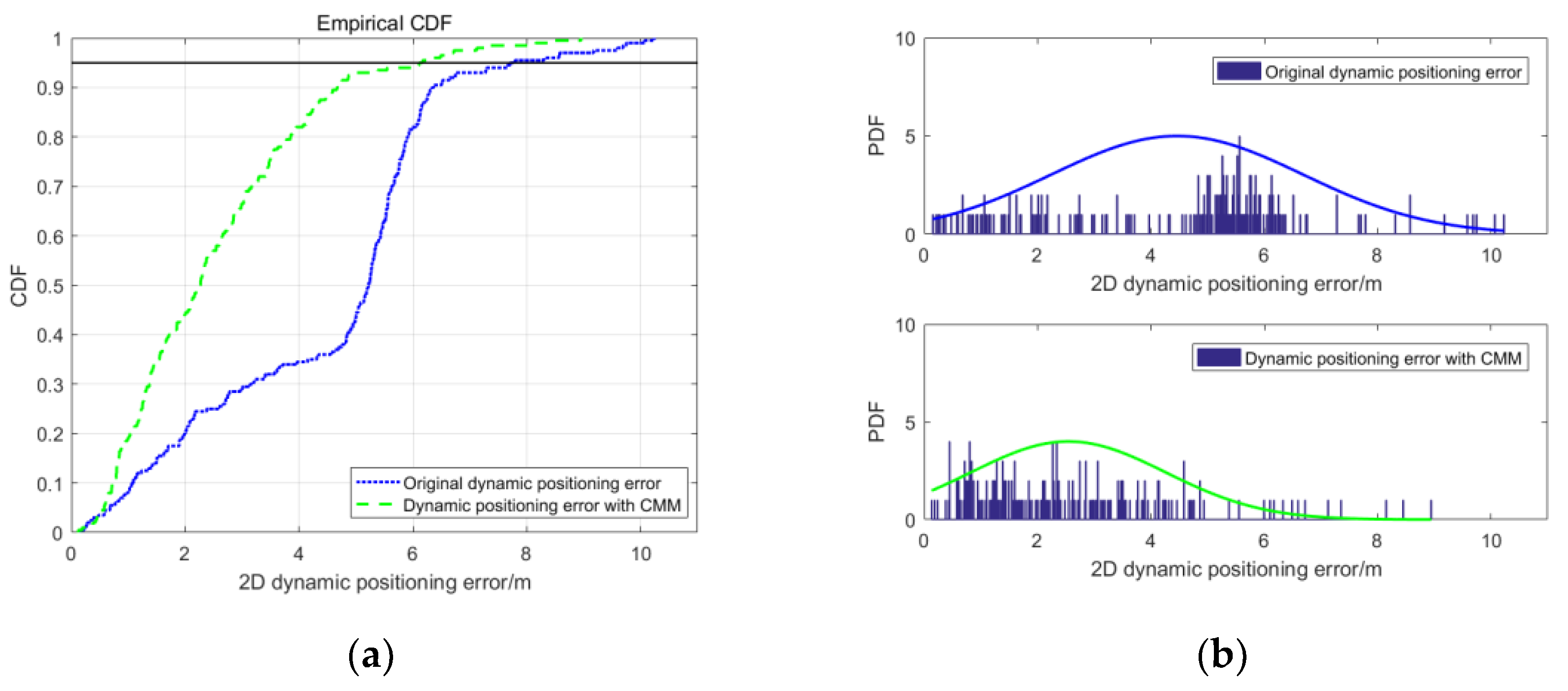
3.2.3. Dynamic Experiment

As shown in Figure 10, during the first 60 s, most of the data collected by the low-cost positioning system and M100 receiver are in the same lane. The results in Figure 10a show that the 2D original positioning error is mainly distributed within 3 m in the first 60 s, with an obvious decrease through CMM correction. After the first 60 s, due to the increase of the vehicle speed, the positioning accuracy is reduced, and the 2D positioning error range is mainly concentrated in 5–8 m, no more than 10.5 m. The dynamic positioning results imply that the positioning accuracy can be effectively improved with CMM correction.

In Figure 10b, it can be seen that the eastward positioning error was effectively reduced through CMM correction. Figure 10c illustrates that the northward positioning error can be also reduced to a certain extent. In addition, in the period of 101–119 s, the northward error is increased, as the circled part ① in Figure 10c indicates. Through the analysis of the vehicle positioning trajectory in this period, as shown in Figure 11, it is consistent with the situation in Figure 3b.

As shown in

Table 5. The MAE and RMSE of dynamic positioning experimental results.

	MAE (m)			RMSE (m)
	East	North	2D	East	North	2D
Original positioning	3.76	1.64	4.46	2.36	1.10	2.22
Positioning with CMM	1.66	1.40	2.49	1.36	1.30	1.68

, the MAE and RMSE of the positioning error results with CMM correction are lower than those of the original positioning error results. The MAE of the 2D positioning error is reduced from 4.46 m to 2.49 m. Compared with the original positioning error, the overall RMSE is reduced by 24.3%. The MAE and RMSE values of the eastward positioning error with the CMM method correction are reduced to 1.66 and 1.36 m, respectively.

The CDF and PDF of the dynamic experimental results are shown in Figure 12. From Figure 12a, the error corresponding to the 95% confidence level is reduced from 8 m to 6 m through CMM correction. The PDF in Figure 12b indicates that most of the original dynamic positioning error is scattered within 6.5 m, mainly concentrated in 4–6.5 m. A small part of the positioning error ranges from 6.5 m to 10 m, and the maximum error does not exceed 11 m. In addition, by utilizing the CMM correction, it can be seen that most of the positioning error is distributed within 4 m. Some positioning error values are in the range of 6–8 m, and the maximum error is no more than 9 m.

The trajectory map of the original GPS positioning, CMM correction positioning and reference positioning in the dynamic scenario is presented in Figure 13. From the roadmap, it can be seen more intuitively that in the test road, the positioning route using CMM is obviously close to the reference route, proving the effectiveness of the proposed method. In addition, the performance and reliability of the designed low-cost positioning system are tested and verified.

The results obtained from the above experiments are satisfactory. In the dynamic experiment, the positioning accuracy with the CMM correction was greatly improved. In terms of cost, the price of the ATK-1218 is only 1.5% of the M100, which greatly reduces the positioning cost. In general, we have the advantages of low cost and complexity in the engineering application of positioning.

4. Conclusions and Future Works

In this paper, an application-oriented CMM method is proposed to improve the vehicular positioning accuracy. A low-cost GPS/BDS integrated positioning system is designed to collect the application-oriented positioning data. To verify the positioning effectiveness, the proposed method is conducted on the positioning data in both static and dynamic environments. In the static experiment, the overall MAE and RMSE are reduced by 9.0 and 4.9%, respectively. The error corresponding to the confidence level of 95% is reduced from 2.3 m to 2 m. The original static positioning error is mainly distributed in the range of 1.8–2.3 m, where it is reduced to the range of 1.6–2 m with the CMM correction. In the dynamic experiment, the overall MAE and RMSE of the proposed method are reduced by 44.2% and 24.3%, respectively. The error corresponding to the 95% confidence level is reduced from 8 m to 6 m. The original dynamic positioning error is mainly concentrated in 4–6.5 m, where it is distributed within 4 m with the CMM correction. The experimental results show that the vehicular positioning performance can be improved effectively by the proposed method in both static and dynamic environments.

For future work, we intend to study the effect of the number of adjacent vehicles on the target vehicle’s localization accuracy. Additionally, we will consider establishing a deep learning model to predict the positioning when the navigation signal is interrupted, and also further modify the positioning with the CMM algorithm, to make the algorithm more suitable for positioning requirements in different environments and scenarios.

References

1. Li, L.; Liu, X.H.; Xiao, W.; Tang, X. Analysis on the Influence of BeiDou Satellite Pseudorange Bias on Positioning. In Proceedings of the 2020 IEEE 3rd International Conference on Information Communication and Signal Processing (ICICSP), Shanghai, China, 12–15 September 2020; pp. 399–404. [Google Scholar]
2. Sathish, N.B.; Krishna, N.K.; Odelu, O. Analysis of Multipath Mitigation Techniques in GNSS for Pseudorange Error Reduction. In Proceedings of the 2019 5th International Conference on Computing, Communication, Control and Automation (ICCUBEA), Pune, India, 19–21 September 2019; pp. 1–5. [Google Scholar]
3. Luo, Y.; Weng, Z.; Qi, Y.; Deng, L.; Yu, W.; Li, F.; James, L.; Zhuang, W.; Miao, M.; Huang, J. Short-Baseline High-Precision DGPS for Smart Snow Blower. IEEE Internet Things 2020, 7, 5033–5041. [Google Scholar] [CrossRef]
4. Li, J.; Gao, J.; Zhang, H.; Qiu, T.Z. RSE-Assisted Lane-Level Positioning Method for a Connected Vehicle Environment. IEEE T. Intell. Transp. 2019, 20, 2644–2656. [Google Scholar] [CrossRef]
5. Wing, M.G.; Eklund, A.; Kellogg, L.D. Consumer-grade global positioning system (GPS) accuracy and reliability. J. For. 2005, 103, 169–173. [Google Scholar] [CrossRef]
6. Jo, K.; Lee, M.; Sunwoo, M. Fast GPS-DR Sensor Fusion Framework: Removing the Geodetic Coordinate Conversion Process. IEEE T. Intell. Transp. 2016, 17, 2008–2013. [Google Scholar] [CrossRef]
7. Henkel, P.; Sperl, A.; Mittmann, U.; Bensch, R.; Färber, P. Precise Positioning of Robots with Fusion of GNSS, INS, Odometry, LPS and Vision. In Proceedings of the 2019 IEEE Aerospace Conference, Big Sky, MT, USA, 2–9 March 2019; pp. 1–6. [Google Scholar]
8. Vu, A.; Ramanandan, A.; Chen, A.; Farrell, J.A.; Barth, M.J. Real-time computer vision/DGPS-aided inertial navigation system for lane-level vehicle navigation. IEEE T. Intell. Transp. 2012, 13, 899–913. [Google Scholar] [CrossRef]
9. Lezki, H.; Yetik, İ.Ş. Localization Using Single Camera and Lidar in GPS-Denied Environments. In Proceedings of the 2020 28th Signal Processing and Communications Applications Conference (SIU), Gaziantep, Turkey, 5–7 October 2020; pp. 1–4. [Google Scholar]
10. Ahmed, H.; Tahir, M. Accurate Attitude Estimation of a Moving Land Vehicle Using Low-Cost MEMS IMU Sensors. IEEE T. Intell. Transp. 2017, 18, 1723–1739. [Google Scholar] [CrossRef]
11. Aono, T.; Fujii, K.; Hatsumoto, S.; Kamiya, T. Positioning of vehicle on undulating ground using GPS and dead reckoning. In Proceedings of the 1998 IEEE International Conference on Robotics and Automation (Cat. No.98CH36146), Leuven, Belgium, 20 May 1998; pp. 3443–3448. [Google Scholar]
12. Mayer, P.; Magno, M.; Berger, A.; Benini, L. RTK-LoRa: High-Precision, Long-Range, and Energy-Efficient Localization for Mobile IoT Devices. IEEE T. Instrum. Meas. 2021, 70, 1–11. [Google Scholar] [CrossRef]
13. Rovira-Garcia, A.; Juan, J.M.; Sanz, J.; González-Casado, G. A Worldwide Ionospheric Model for Fast Precise Point Positioning. IEEE T. Geosci. Remote 2015, 53, 4596–4604. [Google Scholar] [CrossRef] [Green Version]
14. Barbarella, M.; Gandolfi, S.; Poluzzi, L.T.L. Precision of PPP as a Function of the Observing-Session Duration. IEEE T. Aero. Elec. Sys. 2018, 54, 2827–2836. [Google Scholar] [CrossRef]
15. Elsheikh, M.; Noureldin, A.; Korenberg, M. Integration of GNSS Precise Point Positioning and Reduced Inertial Sensor System for Lane-Level Car Navigation. IEEE T. Intell. Transp. 2022, 23, 2246–2261. [Google Scholar] [CrossRef]
16. Chen, L.; Ho, Y. Centimeter-Grade Metropolitan Positioning for Lane-Level Intelligent Transportation Systems Based on the Internet of Vehicles. IEEE T. Ind. Inform. 2019, 15, 1474–1485. [Google Scholar] [CrossRef]
17. Song, Y.X.; Fu, Y.C.; Yu, F.R.; Zhou, L. Blockchain-Enabled Internet of Vehicles with Cooperative Positioning: A Deep Neural Network Approach. IEEE Internet Things 2020, 7, 3485–3498. [Google Scholar] [CrossRef]
18. Ansari, K. Cooperative Position Prediction: Beyond Vehicle-to-Vehicle Relative Positioning. IEEE T. Intell. Transp. 2020, 21, 1121–1130. [Google Scholar] [CrossRef]
19. Rabiee, R.; Zhong, X.H.; Yan, Y.S.; Tay, W.P. LaIF: A Lane-Level Self-Positioning Scheme for Vehicles in GNSS-Denied Environments. IEEE T. Intell. Transp. 2019, 20, 2944–2961. [Google Scholar] [CrossRef]
20. Amini, A.; Vaghefi, R.M.; de la Garza, J.M.; Buehrer, R.M. Improving GPS-based vehicle positioning for Intelligent Transportation Systems. In Proceedings of the 2014 IEEE Intelligent Vehicles Symposium Proceedings, Dearborn, MI, USA, 8–11 June 2014; pp. 1023–1029.
21. Mahmoud, A.; Noureldin, A.; Hassanein, H.S. Integrated Positioning for Connected Vehicles. IEEE T. Intell. Transp. 2020, 21, 397–409. [Google Scholar] [CrossRef]
22. Feng, D.Q.; Wang, C.Q.; He, C.L.; Zhuang, Y.; Xia, X.G. Kalman-Filter-Based Integration of IMU and UWB for High-Accuracy Indoor Positioning and Navigation. IEEE Internet Things 2020, 7, 3133–3146. [Google Scholar] [CrossRef]
23. Liu, K.; Lim, H.B.; Frazzoli, E.; Ji, H.; Lee, V.C.S. Improving Positioning Accuracy Using GPS Pseudorange Measurements for Cooperative Vehicular Localization. IEEE T. Veh. Technol. 2014, 63, 2544–2556. [Google Scholar] [CrossRef]
24. Xu, C.; Wu, H.; Duan, S.H. Constrained Gaussian Condensation Filter for Cooperative Target Tracking. IEEE Internet Things 2022, 9, 1861–1874. [Google Scholar] [CrossRef]
25. Liu, J.; Cai, B.G.; Wang, J. Cooperative Localization of Connected Vehicles: Integrating GNSS With DSRC Using a Robust Cubature Kalman Filter. IEEE T. Intell. Transp. 2017, 18, 2111–2125. [Google Scholar] [CrossRef]
26. Kim, D.; Kim, B.; Chung, T.; Yi, K. Lane-Level Localization Using an AVM Camera for an Automated Driving Vehicle in Urban Environments. IEEE-Asme T. Mech. 2017, 22, 280–290. [Google Scholar] [CrossRef]
27. Deng, L.Y.; Yang, M.; Hu, B.; Li, T.Y.; Li, H.; Wang, C.X. Semantic Segmentation-Based Lane-Level Localization Using Around View Monitoring System. IEEE Sens. J. 2019, 19, 10077–10086. [Google Scholar] [CrossRef]
28. Zhang, Z.H.; Zhao, J.T.; Huang, C.Y.; Li, L. Learning Visual Semantic Map-Matching for Loosely Multi-sensor Fusion Localization of Autonomous Vehicles. IEEE T. Intell. Vehicl. (Early Access) 2022. [Google Scholar] [CrossRef]
29. Cui, D.X.; Xue, J.R.; Zheng, N.N. Real-Time Global Localization of Robotic Cars in Lane Level via Lane Marking Detection and Shape Registration. IEEE T. Intell. Transp. 2016, 17, 1039–1050. [Google Scholar] [CrossRef]
30. Rohani, M.; Gingras, D.; Gruyer, D. A Novel Approach for Improved Vehicular Positioning Using Cooperative Map Matching and Dynamic Base Station DGPS Concept. IEEE T. Intell. Transp. 2016, 17, 230–239. [Google Scholar] [CrossRef]
31. Shen, M.C.; Sun, J.; Peng, H.; Zhao, D. Improving Localization Accuracy in Connected Vehicle Networks Using Rao–Blackwellized Particle Filters: Theory, Simulations, and Experiments. IEEE T. Intell. Transp. 2019, 20, 2255–2266. [Google Scholar] [CrossRef] [Green Version]
32. Du, L.Y.; Ji, J.; Pei, Z.H.; Chen, W. A Novel Error Correction Approach to Improve Standard Point Positioning of Integrated BDS/GPS. Sensors 2020, 20, 6162. [Google Scholar] [CrossRef] [PubMed]
Figure 1. Illustration of biased localization caused by pseudoranges error.
Electronics 11 03258 g001
Figure 2. The overall process of CMM correction positioning.
Electronics 11 03258 g002
Figure 3. The principle of road constraints model. (a) Increase in eastward error; (b) increase in northward error; (c) expanded graph of (a); (d) expanded graph of (b).
Electronics 11 03258 g003
Figure 4. Low-cost positioning system. (a) Hardware design diagram; (b) physical system diagram.
Electronics 11 03258 g004
Figure 5. Software flow diagram.
Electronics 11 03258 g005
Figure 6. The connection of the test equipment.
Electronics 11 03258 g006
Figure 7. Static experimental results. (a) Eastward error; (b) northward error; (c) 2D error.
Electronics 11 03258 g007
Figure 8. Static positioning of the low-cost positioning system.
Electronics 11 03258 g008
Figure 9. The CDF and PDF of 2D static positioning error. (a) CDF; (b) PDF.
Electronics 11 03258 g009
Figure 10. Dynamic experimental results. (a) 2D error; (b) eastward error; (c) northward error.
Electronics 11 03258 g010
Figure 11. 101–119 s time period vehicle positioning trajectory route map.
Electronics 11 03258 g011
Figure 12. The CDF and PDF of 2D dynamic positioning error. (a) CDF; (b) PDF.
Electronics 11 03258 g012
Figure 13. Dynamic positioning result reproduced on Google Earth.
Electronics 11 03258 g013