A No-Reference Quality Assessment Method for Screen Content Images Based on Human Visual Perception Characteristics

Abstract

The widespread application of screen content images (SCIs) has met the needs of remote display and online working. It is a topic that is challenging and worthwhile discussing in research on quality assessment for SCIs. However, existing methods focus on extracting artificial features to predict image quality, which are subjective and incomplete, or lack good interpretability. To overcome these problems, we propose an effective quality assessment method for SCIs based on human visual perceptual characteristics. The proposed method simulates the multi-channel working mechanism of the human visual system (HVS) through pyramid decomposition and the information extraction process of brains with the help of dictionary learning and sparse coding. The input SCIs are first decomposed at multiple scales, and then dictionary learning and sparse coding are applied to the images at each scale. Furthermore, the sparse representation results are analyzed from multiple perspectives. First, a pooling scheme about generalized Gaussian distribution and log-normal distribution is designed to describe the sparse coefficients with and without zero values, respectively. Then the sparse coefficients are used to characterize the energy characteristics. Additionally, the probability of each atom is calculated to describe the statistical property of SCIs. Since the above process only deals with brightness, color-related features are also added to make the model more general and robust. Experimental results on three public SCI databases show that the proposed method can achieve better performance than existing methods.

1. Introduction

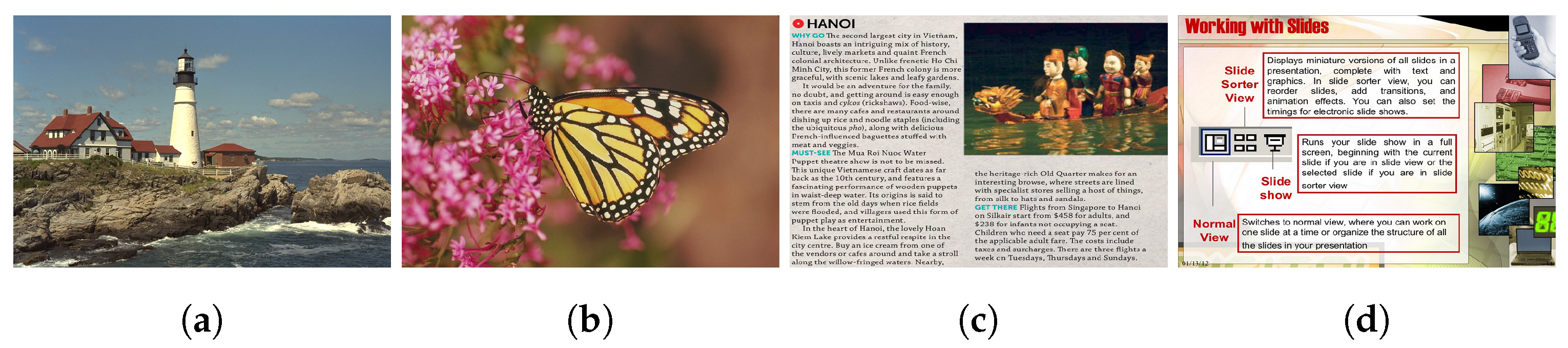
With the rapid development of mobile Internet and multimedia technology, screen content images (SCIs) have been widely used in various interactive scenarios, such as virtual screen sharing, online education, online meetings, cloud computing, and games [1]. Especially in the global outbreak of COVID-19, many normal work and lifestyle cannot be carried out offline in order to prevent crowds from gathering, and people working at home must transmit information through screen content. SCIs generally refer to the interface presented on the screen of a digital viewing device, which usually contain computer-generated content, such as text, computer graphics, etc., as well as content captured by cameras. Examples of traditional natural images and SCIs are shown in Figure 1. In contrast, SCIs typically consist of sharp edges, limited color variations, and repetitive patterns, while natural images usually present smoother edges, rich colors, and complex textures [2,3]. Similar to natural images, in the process of typical multimedia service chain, such as capture, compression, transmission, decompression, and reconstruction, a series of distortions will inevitably be introduced due to the interference of various factors, such as broadband constraint, resolution limitation of hardware devices, and color and contrast changes of remote sharing, which will lead to the decline of the perceived quality of SCIs at the receiving end [4,5,6]. Therefore, as a basic technology in image engineering, image quality assessment (IQA) plays an irreplaceable role in the field of visual information processing and communication, and has profound theoretical significance and important application value.

Generally speaking, IQA methods can be divided into two categories: subjective and objective methods. The former represents the most realistic human perception of images and is the most reliable measure of visual quality among all available means. However, this method is time-consuming and not suitable for real-time processing. Therefore, most studies have focused on the automatic assessment of image quality, aiming to achieve the replacement of human vision in objective ways. Due to its advantages of high efficiency, stability, and integration, the objective research has gradually become a key topic in IQA studies. However, since the modeling of human visual system (HVS) is a very complex process, it is difficult to obtain the characteristics consistent with human vision. In addition, because of the significant differences of perceptual attributes between SCIs and natural images, the existing IQA methods for natural images cannot be directly applied to evaluate the perceptual quality of SCIs [7,8]. Therefore, in order to better meet the needs of practical applications, it is necessary to design an objective and accurate IQA method for SCIs that can fully reflect the characteristics of human visual perception.

2. Related Works

So far, there have been many full-reference (FR) quality assessment studies for SCIs that are able to obtain good performance [9,10,11,12,13,14,15,16]. However, in many practical applications (e.g., remote screen sharing systems and wireless transmission systems), it is often difficult for us to obtain the original versions of distorted SCIs, making such FR methods more limited. Therefore, we focus our research on no-reference (NR) approaches. Existing NR-IQA methods for SCIs can be roughly divided into the following two categories: manual feature extraction-based methods and machine learning-based methods. Gu et al. [17] first proposed a blind quality measurement method (BQMS). Then, a unified framework is concluded and four types of descriptive features are extracted to design an IQA model (SIQE) [18]. Fang et al. [19] utilized histograms to represent statistical luminance and texture features extracted from local normalization and gradient information, respectively. Later on, an improved model (PQSC) [20] was proposed by using a more accurate local ternary patterns (LTP) operator for texture feature extraction and introducing chromatic descriptors. Zheng et al. [21] utilized the variance of local standard deviation to distinguish sharp edge patches (SEPes) and non-SEPes of SCIs. Yang et al. [22] trained stacked autoencoders (SAEs) by a completely unsupervised method to process quality-awareness features extracted from pictorial and textual regions. The problem with these feature extraction-based methods is that those features are obviously subjective and one-sided, and cannot fully reflect the particularity of SCIs. The most typical machine-learning-based approach is the application of neural networks, which provides end-to-end features for better performance. Zuo et al. [23] proposed a framework based on a convolutional neural network (CNN) to predict the quality scores of image patches. Yue et al. [24] attempted to train a network with the entire image and divided the original image into prediction and non-prediction parts according to the internal generation mechanism theory. Chen et al. utilized a “normalization” module consisting of the up-sampling and convolutional layers, aiming to transform the SCIs to have more natural images-like features [25]. Jiang et al. used multi-region local features to generate pseudo-global features, and proposed a novel ranking loss to predict quality scores [26]. Neural networks make up for shortcomings of manual feature extraction methods to a certain extent, but these methods are completely black-box operations that lack interpretability and require a large amount of supervised data, which can easily lead to overfitting if the sample size of the training set is insufficient.

The HVS is critical to the perception of visual signals, and, therefore, we must consider relevant properties of the HVS when designing our model. When we observe the natural world through our eyes, visual signals are transmitted through the lateral geniculate nucleus (LGN) to the primary visual cortex (V1) for visual abstraction. During this process different neurons on the retina and LGN are activated, and these response properties can be successfully explained by the redundancy parsimony principle for interpretation [27]. More theoretical studies have shown that for the perceptual information received by brains from the external world, the primitive visual cortex uses sparse coding to represent them, which is an effective strategy for the distributed representation of neural information populations [28]. In summary, in order to better reflect the characteristics of information processing in HVS, we can use the sparse coding model to simulate the corresponding functions.

The applications of sparse coding in IQA designed for SCIs have also been extensively studied. Existing research shows that algorithms based on sparse coding can achieve data compression more efficiently, and we can use the redundancy property of dictionary to capture intrinsic essential features of signals, which makes it easier to obtain the information contained in signals and improves the effectiveness and completeness of artificial features. Shao et al. [29] proposed a blind quality predictor (BLIQUP-SCI), which was based on the BRISQUE [30] framework, and three features were extracted from both local and global perspectives for SCIs, including gradient magnitude (GM) maps, Gaussian Laplace operator response (GM-LOG) [31], and local binary patterns (LBP). Yang et al. [32] used features based on sparse coding coefficients of the histogram of oriented gradient (HOG) to predict image quality. Zhou et al. [33] achieved a fused representation of images by training local and global feature dictionaries separately. Wu et al. [34] designed a sparse representation model to extract local structural features and combined with global features consisting of luminance statistical features and LBP features. The above algorithms utilize sparse coding to deal with further local and global features, and optimize the artificial features to some extent. To enhance the correlation between features, a tensor domain dictionary-based BIQA method was proposed to better represent SCIs features and the working mechanism of HVS [35].

In summary, current NR-IQA methods for SCIs are mainly considered from two perspectives: on the one hand, the model is applied to extract artificial features directly from the digital representation of images, which is highly subjective and largely depends on the prior knowledge of the quality degradation mechanism of SCIs. On the other hand, neural network-based methods do not have good interpretability, although they can achieve end-to-end training and obtain deep abstract feature representations. Therefore, considering the advantages and limitations of the above two types of approaches, this paper focuses on combining machine learning and manual feature extraction and proposes a NR quality assessment method for SCIs based on human visual perception characteristics. Specifically, we adopt dictionary learning and sparse coding methods in machine learning to simulate the information extraction process of human brains and then analyze the obtained sparse coefficients from multiple perspectives to define artificial features. Compared with previous algorithms, the proposed method extracts more comprehensive features. Additionally, we also introduce a decomposition mechanism of visual channels before simulating brains for sparse analysis to better capture the perception of image details towards human eyes under different viewing conditions. Furthermore, special consideration is given to color information by utilizing a closely related property of color perception as a description of color features. Finally, support vector regression (SVR) is adopted to learn the IQA model from perception features to human subjective scores. Experimental results have shown the performance improvement of the proposed method. In a word, the main contributions of this paper are summarized as follows:

• Dictionary learning and sparse coding techniques were applied to obtain the quality perception characteristics and enhance the effectiveness and objectivity of the feature extraction process. The original samples were transformed into suitable sparse representation, which simplified the learning task and reduced complexity.
• The multi-channel decomposition mechanism of visual system was introduced. Due to the HVS presenting different sensitivity to different frequency signals, details of images under different viewing conditions were captured by introducing multi-scale processing technique, which effectively improved the performance of the proposed model in quality prediction.
• The results of sparse representation were described from several perspectives. Towards the luminance component, a local pooling scheme based on generalized Gaussian distribution and log-normal distribution was designed firstly by analyzing sparse coefficients. Secondly, the overall quality representation was obtained by extracting energy features of the image. Additionally, overall statistical features of SCIs about dictionary atoms were adopted to reduce the information loss in feature aggregation and effectively solve the one-sidedness of artificial features. Finally, we added the image saturation attribute to describe the color information to make extracted features more systematic and complete.

3. No-Reference Quality Assessment Model for Screen Content Images

Considering the characteristics of SCIs and HVS, a no-reference quality assessment model for SCIs is proposed in this paper based on perceptual characteristics of the human visual. The overall framework is shown in Figure 2. On the whole, the proposed method firstly decomposes input images at multiple scales through Gaussian pyramids to simulate the multi-channel working mechanism of HVS. The respective quality contribution is then calculated at each scale, as shown in Figure 3, which contains four stages of dictionary learning, sparse coding, feature extraction, and quality regression. The final quality score Q is obtained by weighted fusion.

3.1. Multi-Scale Processing Technique

The multi-channel mechanism of HVS shows that neurons decompose visual information into different channels, such as color, frequency, orientation, etc. [36]. According to the related research on the phenomenon of contrast sensitivity, human eyes are more sensitive to distortion in the mid-frequency region than in the low-frequency smooth region and the high-frequency texture region [37]. Thus, multi-scale processing is introduced into our algorithm to improve the performance of the quality prediction. The degree of human perception of image details depends on several viewing conditions, such as display resolution, viewing distance, sampling density, etc. To eliminate the effect due to perceptibility differences as much as possible, the multi-scale processing technique simulates the working mechanism of HVS by weighting the relative importance between different scales.

A Gaussian pyramid is a kind of multi-scale representation that applies Gaussian blur and down-sampling several times to generate multiple sets of signals or images at different scales for subsequent processing. The principle of the Gaussian pyramid is shown in Figure 4. In this paper, a Gaussian pyramid is used to process the images, as shown in Figure 2. The proposed model iteratively applies a low-pass filter and down-samples the filtered image by a factor of 2. We denote the index of the original image as scale 1, and the index of the highest scale as scale M, so the result is obtained after a total of $M-1$ iterations. The quality score on the kth scale is denoted as $q_k$, then the final quality prediction score is obtained by combining the results on different scales:

$$Q=\prod _{k=0}^M{\left[q_k\right]}^{{\alpha }_k}$$

(1)

where ${\alpha }_k$ is used to adjust the relative importance of different scales, and we will discuss the values of parameters in detail in Section 4.3.

3.2. Dictionary Learning

Dictionary learning is to capture the most common and essential features among thousands of targets, which can facilitate further processing. A learned representation matrix is used in the general model of dictionary learning to reflect the mapping relationship between the original signal space and the sub-signal space. This important representation matrix is the dictionary, and each column of the dictionary is called an atom. In the implementation, the K-SVD algorithm [38] is adopted for dictionary learning to process input images by using the sequential dictionary update method and completing one dictionary update with K iterations, which has been widely used because of its good performance in various image processing applications. Specifically, we construct an initial dictionary through the dictionary learning objective function model:

$$\underset{D,x_i}{min}\sum _{i=1}^N{∥y_i-D{x}_i∥}_2^2+\lambda \sum {∥x_i∥}_1$$

(2)

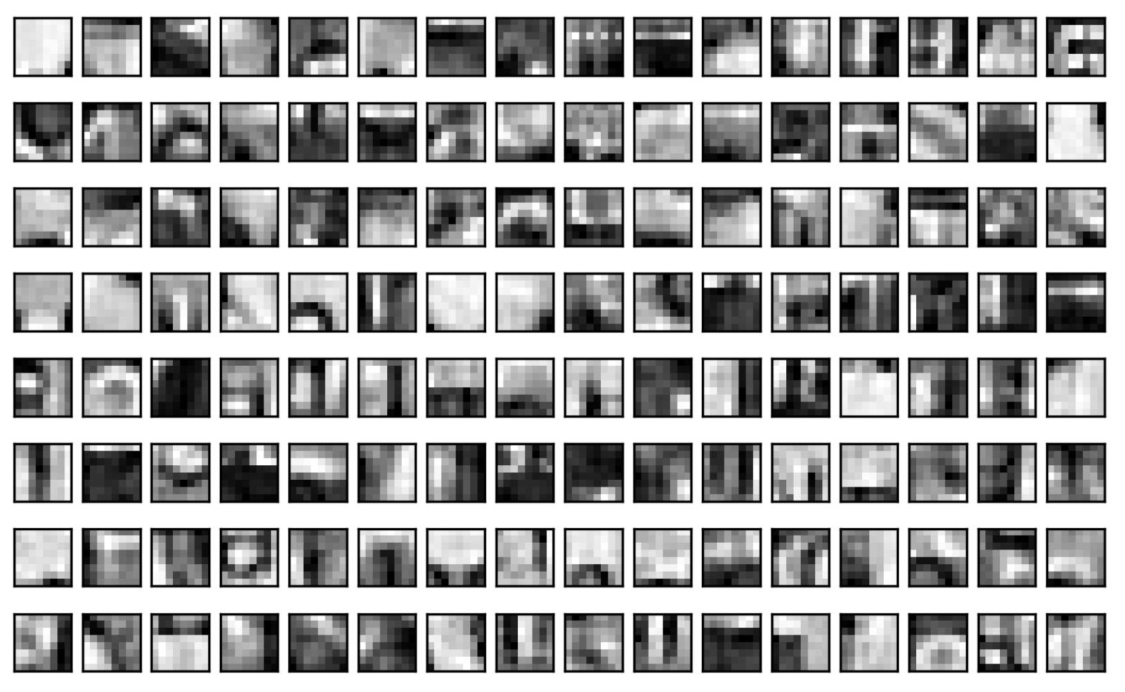
where the first term indicates that the linear combination of the dictionary matrix $D\in {\mathbb{R}}^{p\times K}$ and the sparse representation $x_i\in {\mathbb{R}}^K$ can restore the sample $y_i\in {\mathbb{R}}^p$ as much as possible, and the second cumulative term indicates that the measurement vector $x_i\in {\mathbb{R}}^K$ should be as sparse as possible. The dictionary learned in this paper is shown in Figure 5, where each atom stands for a specific structural feature obtained from the training set, and its corresponding sparse coefficients represent the strength of structural features. Depending on the dictionary, we will obtain different reconstruction coefficients, that is, the values of atoms in the dictionary will directly affect the reconstruction effect of the images.

3.3. Sparse Coding

It has been shown that any given signal is sparse in some transform domain, which means any given signal can be expressed by some dictionary and the corresponding sparse representation [39,40,41,42]. From a biological point of view, sparse coding can be analogous to a neuronal response, while the dictionary atoms being used can be considered as the corresponding active neurons in the retina. Therefore, the existing metric with sparse coefficients can be considered as a measure of degradation of image quality by exploring the different responses given by the same neurons. Sparse coding aims to represent signals with as few useful elements as possible and can, therefore, be well used to describe the receptive fields of simple cells in V1 [28].

Sparse coding simplifies subsequent learning tasks and reduces model complexity by representing the input signal as a sparse linear combination of atoms in a dictionary. In the target dictionary space, sparse reconstruction coefficients can be used to generate effective quality-aware features. In this paper, the optimal solution of Equation (2) is obtained by OMP algorithm. All of the selected atoms are processed orthogonally at each step of decomposition, which enables the faster convergence of the OMP algorithm with the same accuracy requirements. We obtain the sparse coefficients matrix of each patch about dictionary atoms, which will be directly used for feature generation in subsequent modules. According to Equation (3), we can use the learned dictionary $D\in {\mathbb{R}}^{p\times K}$ to perform a sparse representation of the target image:

$$X=argmin{∥x_i∥}_0,s.t.{∥Y-DX∥}_2^2\le T$$

(3)

where $X={\left\{x_i\right\}}_{i=1}^N\in {\mathbb{R}}^{K\times N}$, $Y={\left\{y_i\right\}}_{i=1}^N\in {\mathbb{R}}^{p\times N}$ denotes the input test SCIs, and T denotes the error threshold. We set T to 1 based on experimental comparison results and the effect of different T values on performance will be analyzed in Section 4.3.

3.4. Feature Extraction

After obtaining the sparse representation of images, we can perform feature extraction on the sparse coefficients of all patches, to explore the inherent features for subsequent calculation of quality scores. Considering the characteristics of human visual perception and the particularity of SCIs, five groups of features are selected to form the final feature vector. First, we analyze the sparse coefficient values by adopting different pooling schemes for zero and non-zero values separately to characterize their distribution. Second, we obtain the overall image quality representation by extracting the energy features of the images according to the relationship between sparse coefficient values and energy. Third, We combine the statistical properties of dictionary atoms to obtain the statistical features of images by calculating the probability of atoms in the dictionary. In addition, we add the image saturation property to describe color information of images, making the composition of features more comprehensive and complete. These features will be described one by one below.

3.4.1. Distribution of Sparse Coefficient Values

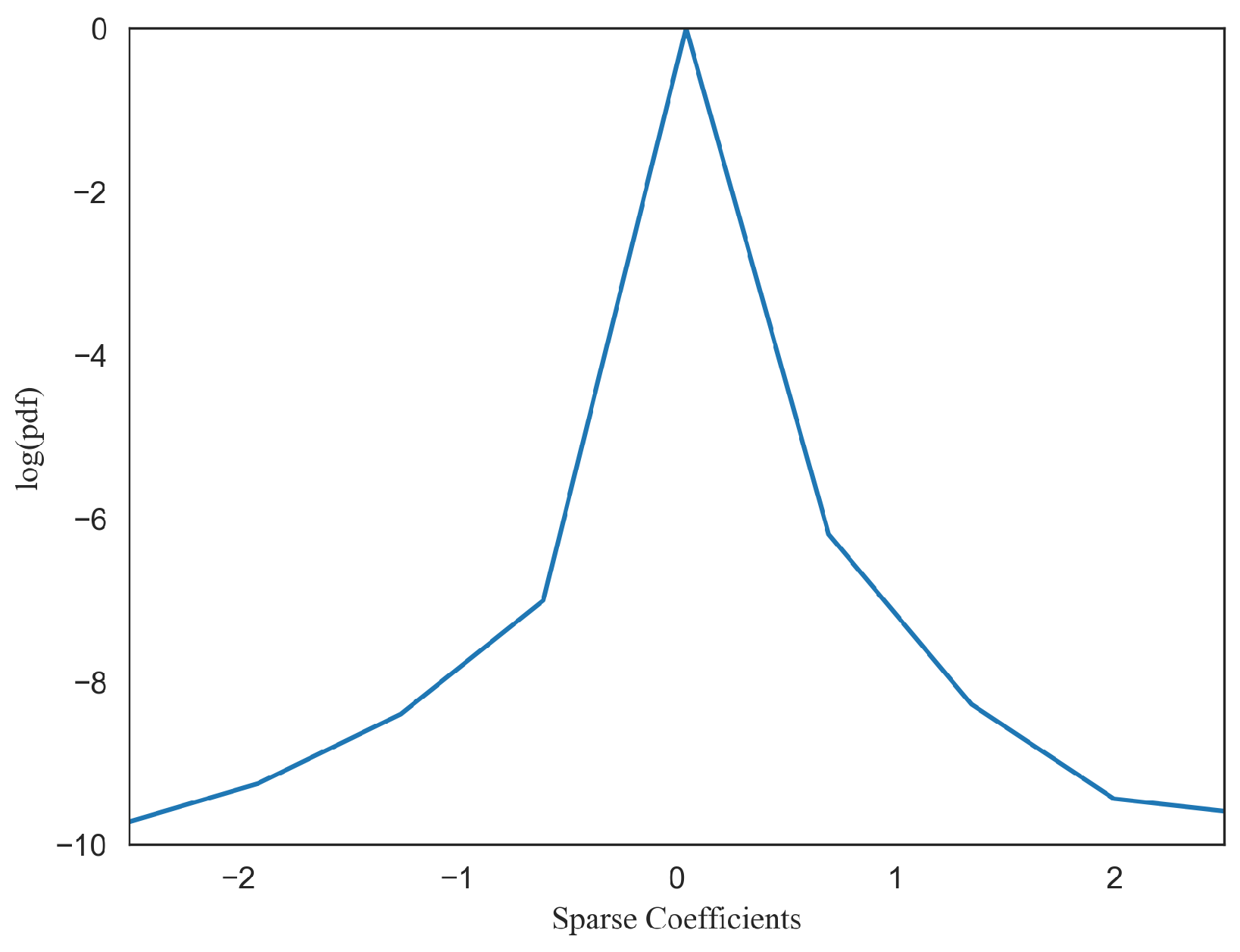
First, we investigate the distribution characteristics of sparse coefficients by analyzing their values to design a suitable pooling scheme. Since the sparse coefficients contain a large number of zero values and a small number of non-zero coefficients with positive and negative values, the process of reconstructing images using a small number of atoms is realized, which greatly improves the efficiency of image reconstruction. Depending on whether the sparse coefficients contain zero values, the frequency distribution histograms show different characteristics. Thus, we will analyze the regularity of sparse coefficients from these two perspectives in this paper. Taking Figure 1c as an example, Figure 6 shows the histogram of all sparse coefficients for atom 1 of the learned dictionary. We can observe that the distribution of sparse coefficients exhibits symmetry and it reaches a very sharp peak at zero with a heavy tail, which can be well approximated by the generalized Gaussian distribution (GGD) [43]. The general definition of GGD is:

$$f\left(x;\alpha ,\beta \right)=\frac{\alpha }{2\times \beta \times \mathsf{\Gamma }\left(\frac{1}{\alpha }\right)}exp-{\left(\frac{\left|x\right|}{\beta }\right)}^{\alpha }$$

(4)

$$\beta =\alpha \sqrt{\frac{\mathsf{\Gamma }\left(\frac{1}{\alpha }\right)}{\mathsf{\Gamma }\left(\frac{3}{\alpha }\right)}}$$

(5)

where $\mathsf{\Gamma }$ represents the gamma function, which is denoted as:

$$\mathsf{\Gamma }\left(z\right)={\int }_0^{\infty }exp\left(-t\right)t^{\left(z-1\right)}\mathrm{d}t,z>0$$

(6)

The GGD model parameters $\left(\alpha ,\beta \right)$ are estimated with the method in [44]. The constant $\alpha$ controls the shape and $\beta$ determines the width of the model. Since the histograms of sparse coefficients and the corresponding GGD model parameters are subject to different distortions, these model parameters can be effectively used for distortion differentiation in quality assessment tasks. 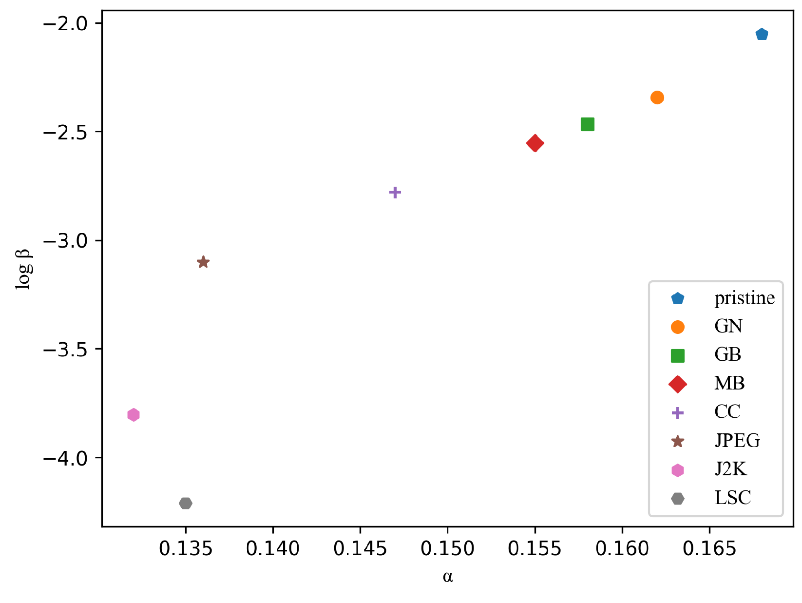Figure 7 shows several sets of GGD parameters fitted by the histogram of sparse coefficients, where the y-axis represents log $\beta$ and the x-axis represents $\alpha$. We can find that there is large discrimination in model parameters for different image distortion types. A similar trend is observed for other atoms. Therefore, the GGD model parameters for each atom of the dictionary form a good set of features for distortion identification, which is denoted as $f^{ggd}$, $f^{ggd}=\left[f_{1,\alpha }^{ggd},f_{1,\beta }^{ggd},\cdots ,f_{K,\alpha }^{ggd},f_{K,\beta }^{ggd}\right]$.

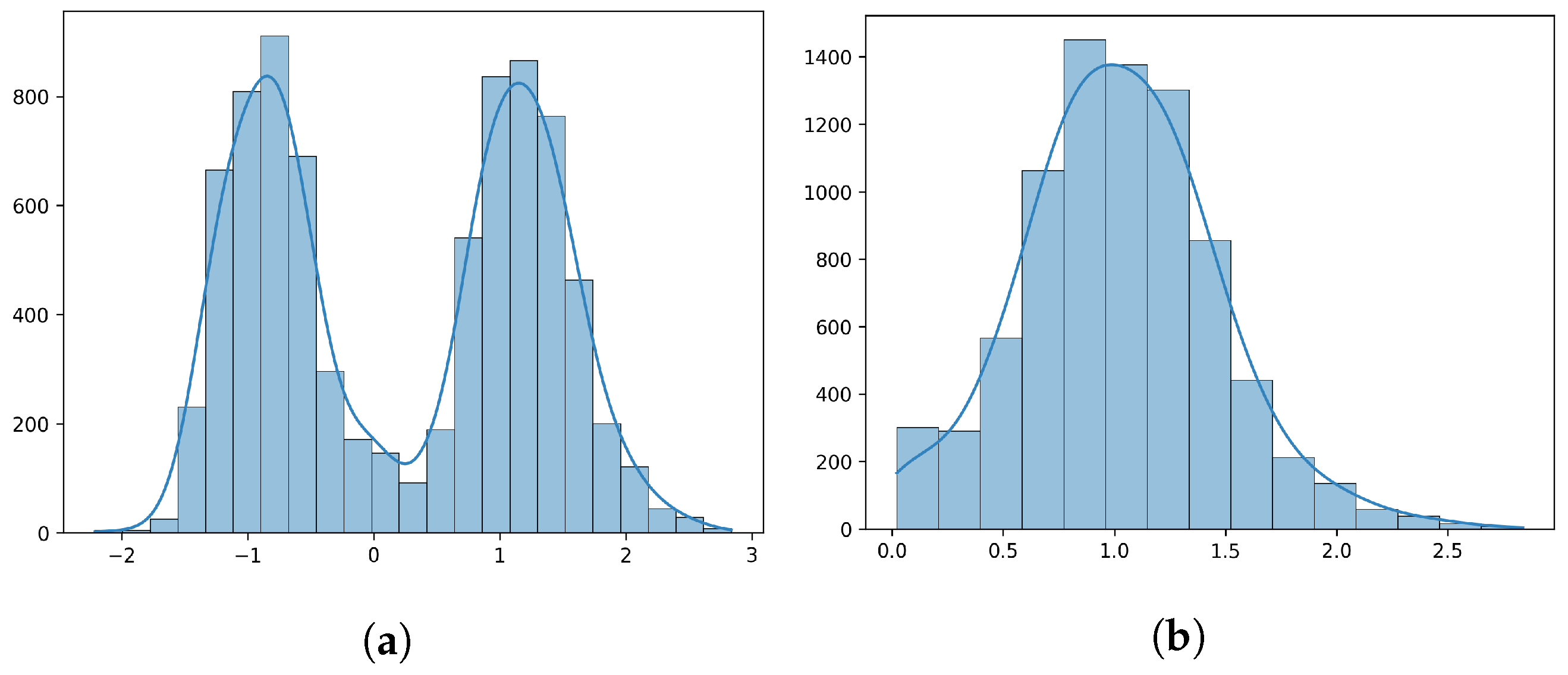
Since atoms with zero coefficients are not involved in the sparse reconstruction of each patch, and test images are reconstructed with partial non-zero sparse coefficient values, the main features of each image can still be accurately characterized [35]. Therefore, we choose non-zero sparse coefficient values as the target object for the next pooling scheme. Figure 8 shows the histograms of sparse coefficients with original and absolute non-zero values.

From Figure 8, it can be seen that values of absolute non-zero sparse coefficients usually follow a log-normal distribution with the probability density function:

$$f\left(x,\mu ,\delta \right)=\frac{1}{\sqrt{2}\pi \delta }exp\left[-\frac{1}{2{\delta }^2}{\left(lnx-\mu \right)}^2\right]$$

(7)

where $\mu$ and $\delta$ are the mean and standard deviation of the logarithm of the variables. Therefore, our statistical feature model can be represented by the mathematical expectation of this log-normal distribution:

$$f^{lnd}=e^{\mu +{\delta }^2/2}$$

(8)

where $f^{lnd}=\left[f_1^{lnd},\cdots ,f_K^{lnd}\right]$ denotes feature vectors of all atoms in the learned dictionary.

3.4.2. Sparse Coefficients and Image Energy

We further consider energy distribution of the overall image. As mentioned above, all atoms in the learned dictionary can be directly used as basic elements to characterize images. Using the dictionary $D\in {\mathbb{R}}^{p\times K}$, each patch can be sparsely represented as follows:

$$Y=DX=\sum _{i=1}^{N}D{x}_i$$

(9)

where N is the patch number and $X\in {\mathbb{R}}^{K\times N}$ denotes the sparse coefficient matrix of $Y\in {\mathbb{R}}^{p\times N}$. Following the derivation in [45], we can compute the energy $\epsilon$ of the sparse coefficients for each image patch as:

$$\epsilon ={∥x_i∥}_2^2=\sum _{j=1}^K{\left|x_{i,j}\right|}^2$$

(10)

where $i\in \left\{0,1,\cdots ,N\right\}$.

Therefore, the energy of each patch can be represented by the corresponding sparse coefficients. If an image is divided into N equal-sized patches, the degree of distortion of the image can be measured by calculating the average energy of all patches. By pooling the energies of all patches, we can obtain the quantity of visual information ${\upsilon }_I$ of an image:

$${\upsilon }_I=\frac{1}{N}\sum _{i=1}^N{\epsilon }_i$$

(11)

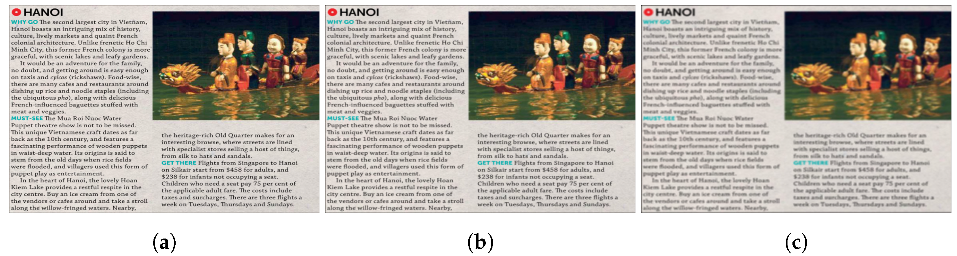
where N is the number of patches contained in the test image. Figure 9 shows three images distorted by Gaussian Blur, and the distortion level increases gradually from Figure 9a–c, which means visual information contained in images is gradually reduced. Through calculation, we can obtain ${\upsilon }_i$ of these three images to be 5.01, 4.73, and 4.31, which is following this decreasing trend.

Since different image patches possess different structural information [46], we need to normalize the energy of each patch with the content change value $\sigma$:

$$q=\frac{\epsilon }{\sigma }$$

(12)

$$\sigma =\frac{1}{P}\sum _{m=1}^P{\left({\lambda }_m-\overline{\lambda }\right)}^2$$

(13)

where P is the number of pixels contained in a patch, ${\lambda }_m$ is the pixel value, and $\overline{\lambda }$ is the average pixel value of an $8\times 8$ image patch. Then, the quality calculation for the entire image can be expressed as:

$$q^{\prime }=\frac{1}{N}\sum _{i=1}^N{q}_i$$

(14)

The calculated results are shown in Figure 9, which are 17447.85, 13406.79, and 9794.33, respectively. We denote this result as the energy feature $f^e$.

3.4.3. Statistical Features of Dictionary Atoms

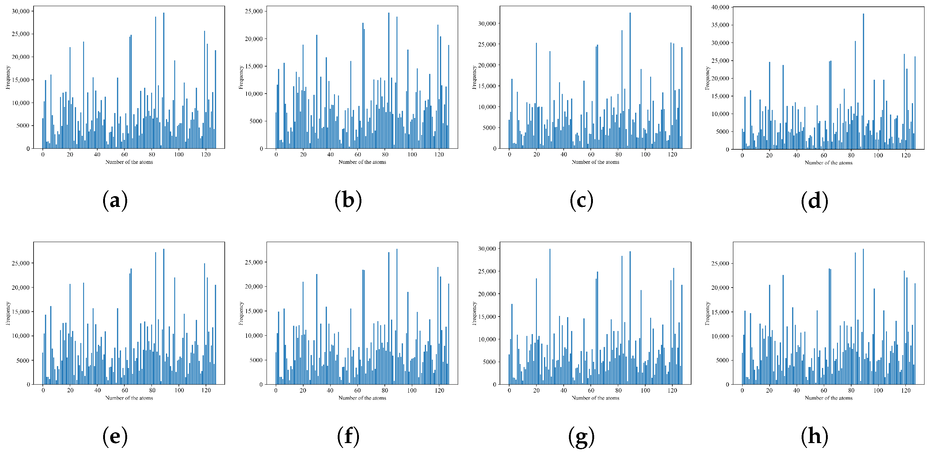
Natural scene statistical information has been widely studied and applied to process natural images, but cannot be directly used for SCIs due to their computer-generated parts. As mentioned above, only the non-zero sparse coefficients are needed to be considered when reconstruction, which means the image reconstruction process can be achieved with different numbers of partial dictionary atoms. We count the occurrence numbers of each atom with different distortion types for Figure 1c,d. The result is shown in Figure 10 and Figure 11. Comparing Figure 10a and Figure 11a, it can be seen that when using the same dictionary to reconstruct images with different contents, the occurrence numbers of each atom in the dictionary are also different. Thus, the statistical features of the dictionary can be used to distinguish different images.

In addition, we further compare and analyze the occurrences of each atom in the dictionary for the same original image with different distortion types. From Figure 11 we can observe that the distribution of occurrences of all atoms has a certain similarity on the whole, but there are still subtle differences due to different types of distortion. This finding shows that statistical features also have the ability to distinguish types of distortion. In summary, there is a certain statistical law in the sparse space of SCIs, which means we can describe the statistical features by counting occurrence numbers of atoms in the dictionary to characterize the changes in quality.

As we know, the occurrence numbers of all atoms are different according to the size of different images. To eliminate this kind of variability, this paper describes the statistical characteristics of SCIs by calculating the probability of atoms. Specifically, the occurrence number of each atom is calculated based on the sparse coefficient vector $X\in {\mathbb{R}}^{K\times N}$, and then the probability value is obtained by normalization process, which is expressed as:

$$f^s=\frac{n_i}{{\sum }_{i=1}^K{n}_i}$$

(15)

where $f^s=\left[f_1^s,\cdots ,f_K^s\right]$ represents the statistical feature vectors of all atoms, and $n_i$ represents the occurrence number of the ith atom in the test image.

3.4.4. Image Color Features

Color information is very attractive to HVS. Existing IQA algorithms for natural images show that the color information contained in an image is also affected to varying degrees when its quality is impaired [47,48,49]. Saturation and hue are properties of color, which are sensitive to color changes and, therefore, are useful to IQA investigations. In the proposed method, we consider the color characteristics of SCIs. We denote an image as $I=\left\{R,G,B\right\}$, thus the image saturation S and hue H can be calculated by:

$$S=1-\frac{3\times M}{U}$$

(16)

$$H={tan}^{-1}\left(\frac{\sqrt{3}\times \left(R-G\right)}{R+G-2B}\right)$$

(17)

where $M=min\left(R,G,B\right)$ and $U=R+G+B$ are denoted as the minimum value and the sum of R, G, and B, respectively. Apparently, the hue values of black and white pixels are zero, which need to be first removed before the color features extraction of input SCIs. Then, calculate the saturation of pixels with hue, and take their mean and quantile values, which are denoted as our image color features $f^c$.

3.5. Quality Regression

In summary, the final vector representation f of this paper is obtained by combining the above five sets of features, where $f=\left[f^{ggd},f^{lnd},f^e,f^s,f^c\right]$. The number of dictionary atoms K is set to 128 in this paper, so each input image contains a total of 517 dimensions in its feature vector.

After obtaining the extracted feature vectors, the support vector regression (SVR) is applied to realize the quality regression at each scale. Specifically, an SVR model trained by the training subset is utilized to obtain the quality score of the testing subset. In this paper, we use SVR with a radial basis function (RBF) kernel as the mapping function to realize the transformation from feature vectors to human subjective quality scores.

4. Results

4.1. SCI Database and Assessment Criteria

In this paper, a total of three public SCI databases are selected for comparative experiments to validate the effectiveness of the proposed method: SIQAD [1], SCID [10], and QACS [50]. SIQAD contains 980 distorted SCIs generated from 20 reference images with a resolution range between $626\times 612$ and $832\times 728$, including a total of seven distortion types with seven degradation levels: GN, GB, MB, CC, JPEG, J2K, and LSC. SCID consists of 40 reference images and 1800 distorted SCIs with a resolution of $1280\times 720$. Each reference image in SCID is degraded by nine distortion types (GN, GB, MB, CC, JPEG, J2K, Color Saturation Change (CSC), High Efficiency Video Coding-Screen Content Coding (HEVC-SCC), and Color Quantization with Dithering (CQD)) and five degradation levels. QACS contains 24 reference images and 492 distorted SCIs with three types of resolutions: $2560\times 1440$, $1920\times 1080$ and $1280\times 720$, and includes two types of distortion: HEVC and SCC.

Meanwhile, to validate the performance of the proposed method, three widely used criteria are employed to calculate the correlation between subjective and objective scores: Pearson Linear Correlation Coefficient (PLCC), Spearman Rank-order Correlation Coefficient (SRCC), and Root Mean Squared Error (RMSE) [51]. PLCC estimates the quality prediction accuracy, SRCC examines the quality prediction monotonicity, and RMSE measures the prediction consistency. In general, higher values of PLCC and SROCC while the lower value of RMSE indicates better performance.

Furthermore, a non-linear logistic regression process was performed to map the dynamic range of the scores from IQA models to a common scale according to the video quality experts group (VQEG):

$$\tilde{Q}={\beta }_1\left[\frac{1}{2}-\frac{1}{1+exp\left[{\beta }_2\left(Q-{\beta }_3\right)\right]}\right]+{\beta }_{4}Q+{\beta }_5$$

(18)

where Q is the objective score calculated by an IQA model, $\tilde{Q}$ is the corresponding mapped score, and ${\beta }_1,{\beta }_2,{\beta }_3,{\beta }_4,{\beta }_5$ are the parameters to be fitted by minimizing the sum of squared differences between the objective and subjective evaluation scores.

In the specific implementation, a dataset is randomly divided into non-overlapping training subset and testing subset, where 80% of the data are selected for training and the remaining 20% for testing. After the optimal model is trained on the training subset, the prediction performance is tested on the test subset. This process is repeated 1000 times and the average values of all prediction results become the measurement of final performance.

4.2. Performance Comparison and Analysis

4.2.1. Overall Performance Comparison

To evaluate the performance of the proposed method, we first compare it with the following FR-IQA methods, which include three classical methods designed for natural images (PSNR, SSIM [52], and GMSD [53]), and eight state-of-the-art methods designed for SCIs (GSS [9], ESIM [10], MDOGS [11], EFGD [12], SFUW [13], CNN-SQE [14], GFM [15], and LGFM [16]).

Table 1. Performance comparison results of different FR-IQA methods on the SIQAD, SCID, and QACS databases.

Method	SIQAD			SCID			QACS
	PLCC	SRCC	RMSE	PLCC	SRCC	RMSE	PLCC	SRCC	RMSE
PSNR	0.5869	0.5608	11.5859	0.7622	0.7512	9.1682	0.861	0.8589	1.1273
SSIM	0.5912	0.5836	11.545	0.7343	0.7146	9.6133	0.8696	0.8683	1.0953
GMSD	0.7387	0.7305	9.6484	0.8337	0.8138	7.8210	0.9019	0.9039	0.9585
GSS	0.8461	0.8359	7.6310	-	-	-	-	-	-
ESIM	0.8788	0.8632	6.8310	0.8630	0.8478	7.1552	-	-	-
MDOGS	0.8839	0.8822	6.6951	-	-	-	-	-	-
EFGD	0.8993	0.8901	6.2595	0.8846	0.8774	6.6044	-	-	-
SFUW	0.8912	0.8800	6.4991	0.8585	0.8281	7.2133	-	-	-
CNN-SQE	0.9042	0.8943	6.1147	0.9147	0.9139	5.7609	-	-	-
GFM	0.8828	0.8735	6.7234	0.8760	0.8759	6.8310	-	-	-
LGFM	-	-	-	0.9023	0.9046	6.1052	-	-	-
Proposed	0.9213	0.9203	5.7965	0.9109	0.9056	6.0682	0.9579	0.9604	0.6839

shows the overall results of various models on three databases, and the best two performance under each criterion are highlighted in boldface.

From Table 1 we can draw the following conclusions. First, compared to the FR-IQA methods for natural images, the methods specially designed for SCIs have better performance in predicting the quality of SCIs, the main reason is that the classical methods do not fully consider the perception characteristics of SCIs. This result also proves once again that SCIs have certain specificity compared with natural images, and the classical methods are no longer suitable for direct application in the quality assessment tasks of SCIs. Second, among the eight methods specially designed for SCIs, two methods, CNN-SQE and LGFM, have better performance than others. Specifically, the basic idea of CNN-SQE is to divide input SCIs into three categories: plain text, computer graphics, and natural images by CNN, and design an edge structure-based quality degradation model that integrates the region size adaptive strategy. LGFM, on the other hand, uses Log-Gabor filters with similarities to HVS to extract features from the luminance component of the reference and distorted SCIs, respectively, and finally combines the measurements of the other two chromaticity components to obtain the final quality score. Although these FR-IQA methods based on features of HVS use the accurate and comprehensive information from reference images, the reference information is not available in most practical applications, limiting the further generalization of these methods. In contract, the proposed method reflects the characteristics of HVS and SCIs by considering the dictionary learning and sparse coding, which presents better performance on three public SCI databases than other FR-IQA methods for SCIs.

Furthermore, we also analyze the proposed method compared to several state-of-the-art NR-IQA methods, including three classical methods designed for natural images (NIQE [54], BRISQUE [30], and GM-LOG [31]), and nine methods designed for SCIs, which include manual feature extraction-based methods (PQSC [20], HRFF [21], Yang [22]) and machine-learning-based methods (Yue [24], PICNN [25], RIQA [26], BLIQUP-SCI [29], TFSR [32], and Bai [35]). The results of the performance comparison are shown in

Table 2. Performance comparison results of different NR-IQA methods on the SIQAD, SCID, and QACS databases.

Method	SIQAD			SCID			QACS
	PLCC	SRCC	RMSE	PLCC	SRCC	RMSE	PLCC	SRCC	RMSE
NIQE	0.3749	0.3568	13.1520	0.3904	0.3712	12.9827	0.4240	0.3701	1.7091
BRISQUE	0.8113	0.7749	8.2565	0.7696	0.7448	9.0143	0.8421	0.8201	1.0959
GM-LOG	0.7608	0.7035	9.2530	0.7883	0.7619	8.6754	0.9002	0.8903	0.9656
PQSC	0.9164	0.9069	5.7080	0.9179	0.9147	5.4793	0.9362	0.9299	0.7746
HRFF	0.852	0.832	7.415	-	-	-	-	-	-
Yang	0.8738	0.8543	6.9335	-	-	-	-	-	-
BLIQUP-SCI	0.7705	0.7990	10.0200	-	-	-	-	-	-
TFSR	0.8618	0.8354	7.4910	0.8017	0.7840	8.8041	-	-	-
Bai	0.9162	0.9090	5.7111	0.8811	0.8730	6.7031	0.9196	0.9123	0.8654
Yue	0.8834	0.8634	6.3971	0.8710	0.8663	6.4123	-	-	-
PICNN	0.896	0.897	6.790	0.827	0.822	8.013	-	-	-
RIQA	0.9107	0.9002	5.8803	-	-	-	-	-	-
Proposed	0.9213	0.9203	5.7965	0.9109	0.9056	6.0682	0.9579	0.9604	0.6839

, with the best two performance are highlighted in boldface.

First, it can be observed that the performance of traditional methods (such as NIQE, BRISQUE, and GM-LOG) are worse than other methods in Table 2, especially NIQE, whose perceptual features based on natural images are quite different from SCIs. Second, most methods based on feature extraction present poor results, and the reason may lie in the subjectivity and one-sidedness of the artificial features extracted by these methods. In contrast, PQSC achieves superior results over other feature extraction-based methods, and it is important that it considers color information that is easily ignored in previous studies. Texture features are extracted by the LTP operator to capture accurate amplitude information of contrast changes, making the extracted features more comprehensive. Third, among the machine learning-based methods, the neural network-based ones avoid the shortcomings of manual feature extraction and achieve better results, but the biggest problem is that they do not reflect the consideration of HVS and lack interpretability. Compared with other methods based on sparse coding, Bai firstly uses tensor decomposition to avoid the loss of color information, and then establishes a macro–micro model to characterize the features, which enhances the correlation among features and provides a systematic mathematical explanation for feature extraction, and, therefore, presents a good result. Finally, results of Table 2 indicate that our method shows a better performance on all three databases, especially on the SIQAD and QACS. Thanks to the introduction of the multi-channel mechanism of HVS, the perception of detailed information at different scales can be captured. Additionally, the proposed method adopts dictionary learning and sparse coding methods in machine learning to simulate the information extraction process of human brains, and analyzes the obtained sparse coefficients from multiple perspectives to define manual features, which are more objective and comprehensive than previous methods. To be specific, we achieve a 9% enhancement in PLCC and SRCC on the SIQAD compared to the experimental results of other methods based on sparse coding.

4.2.2. Performance Comparison of Individual Distortion Type

Then, in order to better validate and refine the experimental results, we will further compare the performance of the three databases according to the different distortion types, as shown in

Table 3. PLCC, SRCC, and RMSE values of the proposed method for different distortion types on the SIQAD, SCID, and QACS databases.

Distortion	SIQAD			SCID			QACS
	PLCC	SRCC	RMSE	PLCC	SRCC	RMSE	PLCC	SRCC	RMSE
GN	0.9422	0.9075	4.6610	0.9615	0.9516	4.0238	-	-	-
GB	0.9211	0.8697	5.7500	0.8711	0.8565	5.6559	-	-	-
MB	0.9217	0.8287	4.9981	0.8746	0.8679	5.6091	-	-	-
CC	0.6708	0.5950	8.3589	0.7895	0.7904	6.1235	-	-	-
JPEG	0.8301	0.8648	4.7057	0.9316	0.8962	6.0986	-	-	-
J2K	0.8800	0.8391	5.5275	0.8868	0.8223	7.7547	-	-	-
LSC	0.8373	0.7975	4.7901	-	-	-	-	-	-
CSC	-	-	-	0.9251	0.9036	3.8344	-	-	-
CQD	-	-	-	0.8287	0.8495	8.2835	-	-	-
HEVC	-	-	-	-	-	-	0.9871	0.9754	0.3561
SCC	-	-	-	0.8845	0.8522	5.8513	0.8957	0.8855	1.0711
Overall	0.9213	0.9203	5.7965	0.9109	0.9056	6.0682	0.9579	0.9604	0.6839

. From the table, we can observe that the proposed method can present satisfactory results on most of the existing distortion types, and can more accurately evaluate and reflect GN, GB, MB, JPEG, and J2K caused quality degradation compared to other types. Although HEVC and SCC are JPEG and blur combined with multiple distortions, which also shows that our method performs well for SCIs with blur and compression distortion. However, the model gives relatively poor test results for CC. For SCIs distorted by CC in the databases, although the impact on the human visual is greater in pictorial regions than in text regions, the overall view shows the opposite result, which means the integrity of the whole image is more susceptible to distortion types such as GN, GB, and MB. In this paper, we extract the quality perception features of the whole image instead of extracting them separately from the pictorial and text regions, which may be the reason for the poor performance of CC.

4.2.3. Performance Analysis of Model Feature Components

To validate the effectiveness of the extracted quality-aware features, we divide them into five groups (distribution features of sparse coefficient values, image energy features, statistical features, and color features, where the distribution features of sparse coefficient values contain both generalized Gaussian distribution and log-normal distribution) and use only the other four groups to learn the quality regression model.

Table 4. Performance results of different features of the proposed method on the SIQAD, SCID and QACS databases.

Database	Criteria	${\mathit{f}}^{\mathit{g}\mathit{g}\mathit{d}-}$	${\mathit{f}}^{\mathit{l}\mathit{n}\mathit{d}-}$	${\mathit{f}}^{\mathit{e}-}$	${\mathit{f}}^{\mathit{s}-}$	${\mathit{f}}^{\mathit{c}-}$	Proposed
SIQAD	PLCC	0.9044	0.9077	0.9113	0.9058	0.9122	0.9213
	SRCC	0.8982	0.9173	0.9098	0.9046	0.9117	0.9203
	RMSE	6.2550	6.3165	6.1368	6.3608	6.1071	5.7965
SCID	PLCC	0.8922	0.9063	0.8993	0.8998	0.8524	0.9109
	SRCC	0.8910	0.9004	0.8944	0.8979	0.8261	0.9056
	RMSE	6.6410	6.2145	6.4323	6.4175	7.6905	6.0682
QACS	PLCC	0.9510	0.9054	0.9328	0.9276	0.9339	0.9579
	SRCC	0.9528	0.8976	0.9312	0.9290	0.9320	0.9604
	RMSE	0.7367	1.0114	0.8588	0.8902	0.8520	0.6839

shows the experimental results, where $f^{e-}$ represents the feature vector without image energy features. Other variables are the same. The proposed method with these five groups of features shows superior performance compared with the method containing only four groups.

4.3. Influencing Factors

In our algorithm, the main factors affecting the performance may come from the following aspects: the base atom size p and the error threshold T need to be optimized during the training process of the dictionary. For the pyramid decomposition process we also need to consider the choice of scales. Therefore, we validate the effect of different parameter settings on the results by comparative experiments.

First, as described in Section 3.2, dictionary atoms and their corresponding sparse coefficients are used to achieve image reconstruction, so the size of atoms will directly affect the size and number of patches in test images and calculation complexity.

Table 5. Performance results of the proposed method with different atom sizes on the SIQAD database.

p	PLCC	SRCC	RMSE
4 × 4	0.9087	0.9107	6.2224
8 × 8	0.9213	0.9203	5.7965
10 × 10	0.9020	0.9033	6.4359
16 × 16	0.8795	0.8881	7.0936

shows the experimental results corresponding to different atom sizes, where p represents the size of each atom in the dictionary. The parameters used in the proposed method finally are highlighted in boldface, and The best performance is shown when the atom size is set to $8\times 8$, which determines our final default value.

In addition, T represents the error threshold defined in Equation (3). According to the features of HVS and sparse coding, if the T value is not suitable, the performance of results will be affected. Increasing T means lower computational complexity, but missing features resulting in worse reconstructed image quality; while decreasing T may cause the features to become similar. According to the experimental results in

Table 6. Performance results of the proposed method with different error thresholds on the SIQAD database.

T	PLCC	SRCC	RMSE
1	0.9213	0.9203	5.7965
5	0.9169	0.9127	5.9483

, we finally set the default value of T to 1.

We also investigate the effect of scales on performance. The results are shown in

Table 7. Performance results of the proposed method with different scales on the SIQAD database.

M	PLCC	SRCC	RMSE
1	0.9108	0.9116	6.1552
3	0.9139	0.9140	6.0498
5	0.9213	0.9203	5.7965

, where M represents scales in the progress of multi-scale processing, that is, the number of down-sampling iterations performed on original images, which indicates how many levels of visual information are included in the model. In practice, different M can be chosen depending on environmental factors and sensitivity to subject details. A too-large M will cause the down-sampled image to exceed the perceptual capacity of HVS, which will have an impact on the stability of the quality prediction. Considering the experimental results in Table 7 and the relevant reference [55], we set M to 5 in our implementation. According to Section 3.1, HVS is more sensitive to medium-scale information than large-scale and small-scale, so we set the weights of different scales ${\alpha }_k$ to [0.15, 0.25, 0.35, 0.20, 0.05], which means to give a larger weight to the intermediate scale and relatively small weight to the large and small scales, which is also the same as the setting of the classic MS-SSIM model.

4.4. Limitations

Through the analysis of the above experimental results, we validate the effectiveness of the proposed method. However, it is undeniable that there are still some shortcomings that need to be improved. First of all, our method can more accurately evaluate and reflect the quality degradation caused by most of the existing distortion types, but it does not present better results for some particular distortion types (such as contrast changes). This may be due to the fact that we have not considered the features of pictorial region and text region separately, which are different to some extent. We will make further improvements to this point in the subsequent research. In addition, the proposed method is different from the traditional artificial feature extraction-based methods, which makes the extracted features more comprehensive and can better reflect the working mechanism of HVS. Our model can also achieve the effect no less than the application of deep learning-based methods. In fact, the research based on deep learning is still a hot spot in current related fields. If more sufficient datasets are available in the future, these methods can also play their roles better.

5. Conclusions

This paper proposes an effective quality assessment model specifically for screen content images. Compared with other existing IQA methods, the proposed method has the following characteristics. Specifically, the method fully considers the perceptual characteristics of the human visual. First, the multi-channel working mechanism of the HVS is simulated by pyramid decomposition in multi-scale processing. Second, the most essential features of input SCIs are extracted by dictionary learning and sparse coding techniques, and the sparse coefficients corresponding to each image patch are obtained to simulate the information extraction mechanism of human brains. Furthermore, these sparse coefficient values and dictionary atoms are analyzed from multiple perspectives. Color features are also added to make the model features completer and more robust. The final quality prediction process is based on the support vector regression. The experimental results on SIQAD, SCID, and QACS databases show that the proposed method can achieve better performance than other IQA methods for SCIs.

References

1. Yang, H.; Fang, Y.; Lin, W. Perceptual quality assessment of screen content images. IEEE Trans. Image Process. 2015, 24, 4408–4421. [Google Scholar] [CrossRef] [PubMed]
2. Wang, S.; Gu, K.; Zeng, K.; Wang, Z.; Lin, W. Objective quality assessment and perceptual compression of screen content images. IEEE Comput. Graph. Appl. 2016, 38, 47–58. [Google Scholar] [CrossRef] [PubMed]
3. Ma, Z.; Wang, W.; Xu, M.; Yu, H. Advanced screen content coding using color table and index map. IEEE Trans. Image Process. 2014, 23, 4399–4412. [Google Scholar] [CrossRef]
4. Yang, A.; Zeng, H.; Chen, J.; Zhu, J.; Cai, C. Perceptual feature guided rate distortion optimization for high efficiency video coding. Multidimens. Syst. Signal Process. 2017, 28, 1249–1266. [Google Scholar] [CrossRef]
5. Ma, S.; Zhang, X.; Zhang, J.; Jia, C.; Wang, S.; Gao, W. Nonlocal in-loop filter: The way toward next-generation video coding? IEEE MultiMedia 2016, 23, 16–26. [Google Scholar] [CrossRef]
6. Yang, Q.; Ma, Z.; Xu, Y.; Yang, L.; Zhang, W.; Sun, J. Modeling the screen content image quality via multiscale edge attention similarity. IEEE Trans. Broadcast. 2019, 66, 310–321. [Google Scholar] [CrossRef]
7. Gu, K.; Wang, S.; Yang, H.; Lin, W.; Zhai, G.; Yang, X.; Zhang, W. Saliency-guided quality assessment of screen content images. IEEE Trans. Multimed. 2016, 18, 1098–1110. [Google Scholar] [CrossRef]
8. Zhang, L.; Li, M.; Zhang, H. Fast intra bit rate transcoding for HEVC screen content coding. IET Image Process. 2018, 12, 738–744. [Google Scholar] [CrossRef]
9. Ni, Z.; Ma, L.; Zeng, H.; Cai, C.; Ma, K.K. Gradient direction for screen content image quality assessment. IEEE Signal Process. Lett. 2016, 23, 1394–1398. [Google Scholar] [CrossRef]
10. Ni, Z.; Ma, L.; Zeng, H.; Chen, J.; Cai, C.; Ma, K.K. ESIM: Edge similarity for screen content image quality assessment. IEEE Trans. Image Process. 2017, 26, 4818–4831. [Google Scholar] [CrossRef]
11. Fu, Y.; Zeng, H.; Ma, L.; Ni, Z.; Zhu, J.; Ma, K.K. Screen content image quality assessment using multi-scale difference of Gaussian. IEEE Trans. Circuits Syst. Video Technol. 2018, 28, 2428–2432. [Google Scholar] [CrossRef]
12. Wang, R.; Yang, H.; Pan, Z.; Huang, B.; Hou, G. Screen content image quality assessment with edge features in gradient domain. IEEE Access 2019, 7, 5285–5295. [Google Scholar] [CrossRef]
13. Fang, Y.; Yan, J.; Liu, J.; Wang, S.; Li, Q.; Guo, Z. Objective quality assessment of screen content images by uncertainty weighting. IEEE Trans. Image Process. 2017, 26, 2016–2027. [Google Scholar] [CrossRef] [PubMed]
14. Zhang, Y.; Chandler, D.M.; Mou, X. Quality assessment of screen content images via convolutional-neural-network-based synthetic/natural segmentation. IEEE Trans. Image Process. 2018, 27, 5113–5128. [Google Scholar]
15. Ni, Z.; Zeng, H.; Ma, L.; Hou, J.; Chen, J.; Ma, K.K. A Gabor feature-based quality assessment model for the screen content images. IEEE Trans. Image Process. 2018, 27, 4516–4528. [Google Scholar] [CrossRef] [PubMed]
16. Guo, H.; Ma, K.K.; Zeng, H. A log-gabor feature-based quality assessment model for screen content images. In Proceedings of the 2019 IEEE International Conference on Image Processing (ICIP), Taipei, Taiwan, 22–25 September 2019; pp. 4499–4503. [Google Scholar]
17. Gu, K.; Zhai, G.; Lin, W.; Yang, X.; Zhang, W. Learning a blind quality evaluation engine of screen content images. Neurocomputing 2016, 196, 140–149. [Google Scholar] [CrossRef] [Green Version]
18. Gu, K.; Zhou, J.; Qiao, J.F.; Zhai, G.; Lin, W.; Bovik, A.C. No-reference quality assessment of screen content pictures. IEEE Trans. Image Process. 2017, 26, 4005–4018. [Google Scholar] [CrossRef]
19. Fang, Y.; Yan, J.; Li, L.; Wu, J.; Lin, W. No reference quality assessment for screen content images with both local and global feature representation. IEEE Trans. Image Process. 2017, 27, 1600–1610. [Google Scholar] [CrossRef] [PubMed]
20. Fang, Y.; Du, R.; Zuo, Y.; Wen, W.; Li, L. Perceptual quality assessment for screen content images by spatial continuity. IEEE Trans. Circuits Syst. Video Technol. 2019, 30, 4050–4063. [Google Scholar] [CrossRef]
21. Zheng, L.; Shen, L.; Chen, J.; An, P.; Luo, J. No-reference quality assessment for screen content images based on hybrid region features fusion. IEEE Trans. Multimed. 2019, 21, 2057–2070. [Google Scholar] [CrossRef]
22. Yang, J.; Zhao, Y.; Liu, J.; Jiang, B.; Meng, Q.; Lu, W.; Gao, X. No reference quality assessment for screen content images using stacked autoencoders in pictorial and textual regions. IEEE Trans. Cybern. 2020, 52, 2798–2810. [Google Scholar] [CrossRef]
23. Zuo, L.; Wang, H.; Fu, J. Screen content image quality assessment via convolutional neural network. In Proceedings of the 2016 IEEE International Conference on Image Processing (ICIP), Phoenix, AZ, USA, 25–28 September 2016; pp. 2082–2086. [Google Scholar]
24. Yue, G.; Hou, C.; Yan, W.; Choi, L.K.; Zhou, T.; Hou, Y. Blind quality assessment for screen content images via convolutional neural network. Digit. Signal Process. 2019, 91, 21–30. [Google Scholar] [CrossRef]
25. Chen, J.; Shen, L.; Zheng, L. Naturalization module in neural networks for screen content image quality assessment. IEEE Signal Process. Lett. 2018, 25, 1685–1689. [Google Scholar] [CrossRef]
26. Jiang, X.; Shen, L.; Yu, L.J. No-reference screen content image quality assessment based on multi-region features. Neurocomputing 2020, 386, 30–41. [Google Scholar] [CrossRef]
27. Winkler, S. Digital Video Quality: Vision Models and Metrics; John Wiley & Sons: Hoboken, NJ, USA, 2005. [Google Scholar]
28. Olshausen, B.A.; Field, D.J. Sparse coding with an overcomplete basis set: A strategy employed by V1? Vis. Res. 1997, 37, 3311–3325. [Google Scholar] [CrossRef] [Green Version]
29. Shao, F.; Gao, Y.; Li, F.; Jiang, G. Toward a blind quality predictor for screen content images. IEEE Trans. Syst. Man Cybern. Syst. 2017, 48, 1521–1530. [Google Scholar] [CrossRef]
30. Mittal, A.; Moorthy, A.K.; Bovik, A.C. No-reference image quality assessment in the spatial domain. IEEE Trans. Image Process. 2012, 21, 4695–4708. [Google Scholar] [CrossRef]
31. Xue, W.; Mou, X.; Zhang, L.; Bovik, A.C.; Feng, X. Blind image quality assessment using joint statistics of gradient magnitude and Laplacian features. IEEE Trans. Image Process. 2014, 23, 4850–4862. [Google Scholar] [CrossRef]
32. Yang, J.; Liu, J.; Jiang, B.; Lu, W. No reference quality evaluation for screen content images considering texture feature based on sparse representation. Signal Process. 2018, 153, 336–347. [Google Scholar] [CrossRef]
33. Zhou, W.; Yu, L.; Zhou, Y.; Qiu, W.; Wu, M.W.; Luo, T. Local and global feature learning for blind quality evaluation of screen content and natural scene images. IEEE Trans. Image Process. 2018, 27, 2086–2095. [Google Scholar] [CrossRef]
34. Wu, J.; Xia, Z.; Zhang, H.; Li, H. Blind quality assessment for screen content images by combining local and global features. Digit. Signal Process. 2019, 91, 31–40. [Google Scholar] [CrossRef]
35. Bai, Y.; Zhu, Z.; Jiang, G.; Sun, H. Blind quality assessment of screen content images via macro-micro modeling of tensor domain dictionary. IEEE Trans. Multimed. 2020, 23, 4259–4271. [Google Scholar] [CrossRef]
36. Mandal, D.; Panetta, K.; Agaian, S. Human visual system inspired object detection and recognition. In Proceedings of the 2012 IEEE International Conference on Technologies for Practical Robot Applications (TePRA), Woburn, MA, USA, 23–24 April 2012; pp. 145–150. [Google Scholar]
37. Campbell, F.W.; Robson, J.G. Application of Fourier analysis to the visibility of gratings. J. Physiol. 1968, 197, 551. [Google Scholar] [CrossRef]
38. Aharon, M.; Elad, M.; Bruckstein, A. K-SVD: An algorithm for designing overcomplete dictionaries for sparse representation. IEEE Trans. Signal Process. 2006, 54, 4311–4322. [Google Scholar] [CrossRef]
39. Kong, S.; Wang, D. A dictionary learning approach for classification: Separating the particularity and the commonality. In Proceedings of the European Conference on Computer Vision, Florence, Italy, 7–13 October 2012; pp. 186–199. [Google Scholar]
40. Harandi, M.; Hartley, R.; Shen, C.; Lovell, B.; Sanderson, C. Extrinsic methods for coding and dictionary learning on Grassmann manifolds. Int. J. Comput. Vis. 2015, 114, 113–136. [Google Scholar] [CrossRef] [Green Version]
41. Jiang, Z.; Lin, Z.; Davis, L.S. Label consistent K-SVD: Learning a discriminative dictionary for recognition. IEEE Trans. Pattern Anal. Mach. Intell. 2013, 35, 2651–2664. [Google Scholar] [CrossRef] [PubMed]
42. Pham, D.S.; Venkatesh, S. Joint learning and dictionary construction for pattern recognition. In Proceedings of the 2008 IEEE Conference on Computer Vision and Pattern Recognition, Anchorage, AK, USA, 23–28 June 2008; pp. 1–8. [Google Scholar]
43. Shabeer, P.M.; Bhati, S.; Channappayya, S.S. Modeling sparse spatio-temporal representations for no-reference video quality assessment. In Proceedings of the 2017 IEEE Global Conference on Signal and Information Processing (GlobalSIP), Montreal, QC, Canada, 14–16 November 2017; pp. 1220–1224. [Google Scholar]
44. Sharifi, K.; Leon-Garcia, A. Estimation of shape parameter for generalized Gaussian distributions in subband decompositions of video. IEEE Trans. Circuits Syst. Video Technol. 1995, 5, 52–56. [Google Scholar] [CrossRef]
45. Li, L.; Wu, D.; Wu, J.; Li, H.; Lin, W.; Kot, A.C. Image sharpness assessment by sparse representation. IEEE Trans. Multimed. 2016, 18, 1085–1097. [Google Scholar] [CrossRef]
46. Wu, J.; Shi, G.; Zhang, M.; Chen, G. Visual information measurement with quality assessment. In Proceedings of the 2016 Visual Communications and Image Processing (VCIP), Chengdu, China, 27–30 November 2016; pp. 1–4. [Google Scholar]
47. Lee, D.; Plataniotis, K.N. Toward a no-reference image quality assessment using statistics of perceptual color descriptors. IEEE Trans. Image Process. 2016, 25, 3875–3889. [Google Scholar] [CrossRef]
48. Su, C.C.; Cormack, L.K.; Bovik, A.C. Color and depth priors in natural images. IEEE Trans. Image Process. 2013, 22, 2259–2274. [Google Scholar] [PubMed]
49. Ruderman, D.L.; Cronin, T.W.; Chiao, C.C. Statistics of cone responses to natural images: Implications for visual coding. JOSA A 1998, 15, 2036–2045. [Google Scholar] [CrossRef] [Green Version]
50. Wang, S.; Gu, K.; Zhang, X.; Lin, W.; Zhang, L.; Ma, S.; Gao, W. Subjective and objective quality assessment of compressed screen content images. IEEE J. Emerg. Sel. Top. Circuits Syst. 2016, 6, 532–543. [Google Scholar] [CrossRef]
51. Video Quality Experts Group. Final report from the video quality experts group on the validation of objective models of video quality assessment. In Proceedings of the VQEG Meeting, Ottawa, ON, Canada, 13–17 March 2000. [Google Scholar]
52. Wang, Z.; Bovik, A.C.; Sheikh, H.R.; Simoncelli, E.P. Image quality assessment: From error visibility to structural similarity. IEEE Trans. Image Process. 2004, 13, 600–612. [Google Scholar] [CrossRef] [Green Version]
53. Xue, W.; Zhang, L.; Mou, X.; Bovik, A.C. Gradient magnitude similarity deviation: A highly efficient perceptual image quality index. IEEE Trans. Image Process. 2013, 23, 684–695. [Google Scholar] [CrossRef] [PubMed] [Green Version]
54. Mittal, A.; Soundararajan, R.; Bovik, A.C. Making a “completely blind” image quality analyzer. IEEE Signal Process. Lett. 2012, 20, 209–212. [Google Scholar] [CrossRef]
55. Wang, Z.; Simoncelli, E.P.; Bovik, A.C. Multiscale structural similarity for image quality assessment. In Proceedings of the The Thrity-Seventh Asilomar Conference on Signals, Systems & Computers, Pacific Grove, CA, USA, 9–12 November 2003; Volume 2, pp. 1398–1402. [Google Scholar]
Figure 1. Examples of traditional natural images and screen content images. (a,b): natural images from LIVE. (c,d): screen content images from SIQAD.
Electronics 11 03155 g001
Figure 2. The framework of the proposed IQA method for SCIs. L2↓: down-sampling by factor 2 with low-pass filter. q1, q2, q3, q4, and q5: quality score of scale 1, 2, 3, 4, and 5. ⊗: weighted fusion.
Electronics 11 03155 g002
Figure 3. The flowchart of image processing at each scale.
Electronics 11 03155 g003
Figure 4. Diagram of the Gaussian pyramid principle.
Electronics 11 03155 g004
Figure 5. The learned dictionary of the training set by using the K-SVD algorithm.
Electronics 11 03155 g005
Figure 6. Histogram of all sparse coefficients for atom 1 of the learned dictionary.
Electronics 11 03155 g006
Figure 7. Distortion discrimination based on the GGD parameters fitted by the histogram of sparse coefficients for atom 1 of the learned dictionary. The legend represents the pristine image and the corresponding distortion type for each set of parameters, including Gaussian Noise (GN), Gaussian Blur (GB), Motion Blur (MB), Contrast Change (CC), JPEG compression (JPEG), JPEG2000 compression (J2K), and Layer Segmentation based Coding (LSC).
Electronics 11 03155 g007
Figure 8. Histogram of non-zero sparse coefficients for atom 1 of the learned dictionary. (a) coefficients with non-zero values, (b) coefficients with absolute non-zero values.
Electronics 11 03155 g008
Figure 9. The quantity of visual information contained in images with different distortion levels, the distortion levels from (ac) increase gradually. (a) υ I = 5.19, q’ = 17447.85, (b) υ I = 4.62, q’ = 13406.79, (c) υ I = 4.32, q’ = 9794.33.
Electronics 11 03155 g009
Figure 10. Histograms of occurrence number of each atom for image in Figure 1c with different distortion types. (a) Pristine image, (b) GN, (c) GB, (d) MB, (e) CC, (f) JPEG, (g) J2K, (h) LSC.
Electronics 11 03155 g010
Figure 11. Histograms of occurrence number of each atom for image in Figure 1d with different distortion types. (a) Pristine image, (b) GN, (c) GB, (d) MB, (e) CC, (f) JPEG, (g) J2K, and (h) LSC.
Electronics 11 03155 g011