Risk-Based Capacitor Placement in Distribution Networks

Abstract

In this paper, the problem of sizing and placement of constant and switching capacitors in electrical distribution systems is modelled considering the load uncertainty. This model is formulated as a multicriteria mathematical problem. The risk of voltage violation is calculated, and the stability index is modelled using fuzzy logic and fuzzy equations. The instability risk is introduced as the deviation of our fuzzy-based stability index with respect to the stability margin. The capacitor placement objectives in our paper include: (i) minimizing investment and installation costs as well as loss cost; (ii) reducing the risk of voltage violation; and (iii) reducing the instability risk. The proposed mathematical model is solved using a multi-objective version of a genetic algorithm. The model is implemented on a distribution network, and the results of the experiment are discussed. The impacts of constant and switching capacitors are assessed separately and concurrently. Moreover, the impact of uncertainty on the multi-objectives is determined based on a sensitivity analysis. It is demonstrated that the more the uncertainty is, the higher the system cost, the voltage risk and the instability risk are.

1. Introduction

The most important step in using capacitive banks in electric distribution networks is technical and economic study to determine their proper location and capacity. Undoubtedly, without accurate knowledge and optimization studies, the potential capabilities of this equipment in distribution networks and the resulting technical and economic benefits cannot be achieved. There are several reasons for using capacitors in a network. One of the most important effects of capacitors in distribution networks, which has been studied in almost all papers in recent years, is to reduce energy losses and increase the capacity available to feeders [1,2,3]. Moreover, in many papers, in addition to the effect of a capacitor on energy losses, its effect on improving the voltage profile has also been considered [4,5]. In some papers, the effect of capacitance on the network power factor correction has been discussed [6,7]. In a number of other papers, the planning for the installation of capacitors with switching capability without the presence of voltage regulators [8] and also in its presence [9] has been studied. In some papers, such as [10], in addition to reducing losses due to capacitance in the distribution network, special attention has been paid to minimizing voltage deviation. Due to the importance of the effect of the presence of nonlinear loads on the total harmonic distortion parameter (THD) in the electrical energy distribution network, this issue has been studied in many papers, including [11,12]. In addition, from the point of view of improving voltage stability indices and reliability, the capacitor placement process has been the focus of a number of papers [12,13].

This paper aims to solve the problem of locating fixed and switching capacitors in the presence of uncertainties. In modeling this problem, in addition to minimizing the initial investment costs of capacitors and energy losses and improving economic efficiency, reducing the technical risks due to the presence of uncertainties in the system has also been considered. Technical risks include bus overvoltage and network instability in the range of boundary values. The mathematical model of the problem is formulated based on optimization with multiple criteria, and a special edition of the genetic algorithm is used to search for efficient answers in the designed model.

The innovation presented in this paper is based on the fact that uncertainty in consumer load data is modeled using the concepts of fuzzy numbers. In addition, after load modeling, the Backward–Forward Sweep Load Flow required for the calculation of losses and other network parameters is modified based on fuzzy numbers. Maximum and minimum allowable voltage level values are used to determine the amount of voltage risk. Another goal that has been studied in this paper is loadability in the electric distribution system. We define an index for this parameter in the presence of uncertainty and calculate it based on the concepts and fuzzy equations of this index. Crossing this index over the stability boundary is defined as the risk of instability.

The three desired objective functions, namely the economic objective function, the voltage risk and the instability risk, are solved using a multi-objective evolutionary algorithm. In this optimization problem, fixed and switching capacitors are used simultaneously to reduce all target functions.

2. An Overview of the Concepts of Risk and Uncertainty

The IEEE standard dictionary provides a clear definition consistent with the main rules governing risk and security system evaluation in reference [14]. In this dictionary, the risk associated with an event is defined as “the simple product of the probability and consequence” of the event. In addition, risk can be seen as the risk of the expected value of the outcome [15]. The concepts related to risk and uncertainty used in this article are briefly described below:

2.1. Technical Risks

The technical risks considered in this paper include two types of risks such as the risk of voltage violation from the permitted range and also the risk of voltage stability violation (voltage instability risk).

2.2. Voltage Violation Risk

The lower and upper limits of voltage in a power network are defined by definite minimum and maximum voltage numbers. Any violation of this voltage range will result in the risk of voltage violation.

2.3. Risk of Voltage Instability

The IEEE’s definition of voltage stability is the ability of a power system to maintain a constant voltage in all system loads after a disturbance occurs in certain operating conditions. Disturbance may be a sudden outage of one of the pieces of equipment or a gradual increase in load. When the electric power transferred to the load is increasing in order to supply the added load and both components, i.e., power and voltage, remain controllable, the power system will be voltage stable, and if the system can transfer the electric load but the voltage is lost, the system voltage is unstable.

Voltage collapse occurs when the increase in load causes the voltage to become uncontrollable in a specific area of the power system. Therefore, voltage instability in its nature is a regional phenomenon, which can turn into a general voltage collapse without a quick response.

2.4. Load Uncertainty Risk

Determining the behavior and mathematical model of the load is one of the most basic and difficult problems in the studies of the electrical energy distribution system. In fact, awareness of the nature and behavior of load is the first necessary condition for studying and analyzing electrical energy systems. In studies such as stability, load distribution, loss reduction, etc., which are among the most important system studies, correct load modeling plays a valuable role, and any carelessness in these results will create anomalies that have unfortunate consequences for design and study.

Considering the large number of load points in distribution networks, installing measuring equipment in all these points is not cost-effective from an economic point of view. Therefore, the amount of load at consumption points is usually determined by applying load estimation methods, which is always associated with uncertainty. Some of the reasons for the uncertainty of load modeling are: the large number of devices that make up the load, the lack of access to the information of the users’ devices, the lack of correct information about consumption, the change in the composition of the load with the change of day, week, season and weather and the lack of accurate characteristics of the consumer devices, especially for large voltage and frequency changes.

3. Load Modeling

One of the most important and of course the most difficult steps in conducting research in electrical energy distribution systems is to obtain the load information of the bus networks under study. The amount of load is usually determined using load estimation methods, which is always accompanied by uncertainty. Different methods have been used in modeling uncertainty. The first proposed method in uncertainty analysis with probabilistic load distribution is presented in [16]. In this method, the grid is represented by the DC model, and the traditional load distribution is performed assuming that the bus loads are independent of each other. Reference [17] upgrades this model for normal, short-term and long-term operating conditions. Reference [18] has used the point estimation method and studies on networks with several wind farms with different degrees of dependence. Among the proposed methods, the Monte Carlo simulation is the most comprehensive tool that allows modeling of various uncertainties in load distribution studies. This method, despite the advantages mentioned, is not suitable for implementation in real networks due to its long execution time. In recent years, fuzzy set theory has been used in mathematical modeling of uncertainties. One of the important properties of fuzzy theory is the ease of performing calculations compared to probabilistic methods, which has made the practical application of this theory attractive and widespread.

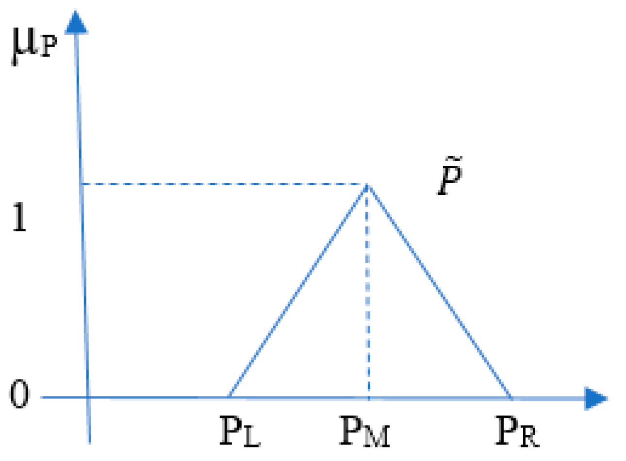
In this paper, uncertainty in distribution network load is modeled using fuzzy numbers. Power consumption at each load point is described as a triangular fuzzy number such as Figure 1. Each triangular fuzzy number has three parameters (P_L, P_M, P_R) and shows that the expected load is around P_M but not less than P_L and not more than P_R. If the estimated power at a load point is P₀ with maximum error e₁ and e₂, the fuzzy number parameters corresponding to that load point can be obtained using the following equations:

$$P_L=\left(1-e_1\right)P_0$$

(1)

$$P_M=P_0$$

(2)

$$P_R=\left(1+e_2\right)P_0$$

(3)

Therefore, the triangular membership function of load can be defined mathematically as follows:

$${\mu }_P=\{\begin{array}{c}0, P\le P_L or P\ge P_R\\ \frac{P-P_L}{P_M-P_L}, P_L<P<P_M \\ \frac{P_R-P}{P_R-P_M}, P_M<P<P_R \end{array}$$

(4)

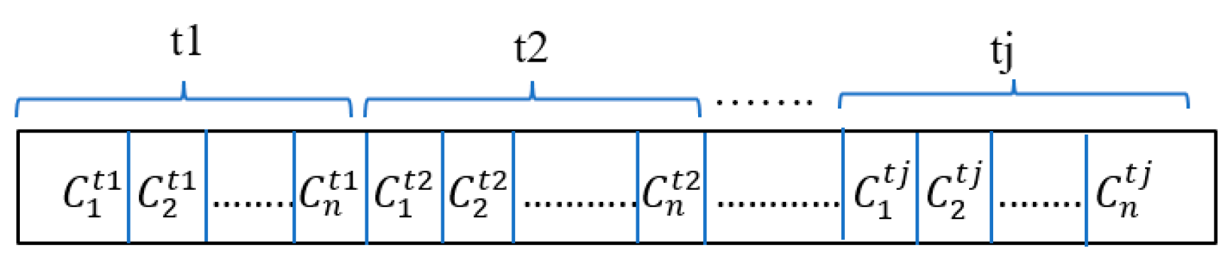
Momentary changes are another characteristic of load in a real distribution network. Therefore, for accurate load modeling, the use of a time-varying model has been proposed. Given the model of hourly load changes, the volume of calculations and, consequently, the time required to perform the simulation to reduce the complexity of the problem, these changes can be classified into certain levels, called the piece Load Duration Curve (LDC).

4. Voltage Risk Modeling

After modeling the load as a triangular fuzzy number, the load distribution based on the fuzzy numbers proposed in [19] is used to determine the electrical parameters of the network. By load modeling and load flow in fuzzy, the whole network model is transferred to the fuzzy domain. Therefore, the voltage of the nodes will also be fuzzy numbers. In Figure 2, the node voltage k is represented as a triangular fuzzy number. In this figure, the allowable upper and lower voltage limits are also shown as definite numbers V_max and V_min, respectively.

Voltage constraint in the fuzzy domain is defined as follows:

$$V_{min}\tilde{\le } {\tilde{V}}_k \tilde{\le }{V}_{max}$$

(5)

Equation (5) is fuzzy, and there is no definite answer for observing or not observing it, but the non-observance of this limitation can be determined with a degree of possibility as follows [19]:

$$S_{V_k}=\frac{A_{ol}+A_{or}}{A_i+A_{ol}+A_{or}}$$

(6)

where $A_i$ is the area under the voltage membership function in the range between the upper and lower voltage limits. $A_{ol}$ and $A_{or}$ are also areas below the voltage membership function that are less than Vmin and more than Vmax, respectively. Fuzzy constraint basically means that with a degree of possibility $S_{V_k}$, the voltage constraint at node k will be violated. As can be seen, by changing the fuzzy number parameter ${\tilde{V}}_k$, the ratio between the areas)$A_i+A_{ol}+A_{or}$ (and) $A_{ol}+A_{or})$ will change, and as a result the degree of possibility will also change.

5. Instability Risk Analysis

In this section, we firstly present the approach to calculate the voltage stability index taking into account the uncertainty. Then, we discuss the network loadability constraint modeling.

Various stability indexes have been proposed for stability analysis in the energy distribution network. Jameson et al. [20] calculated an index for voltage stability based on a single-transmission system. This index is calculated based on the active and reactive load power of the bus [21]. Using the Thevenin theorem, a real network is modeled into a single transfer system [22,23]. In [24], it provides the stability index for a two-bus system and then upgrades this index for use in a real network. In all these models, the stability index is calculated assuming the load information is definite. In this paper, we have tried to calculate the stability index by considering fuzzy uncertainty in the form of fuzzy numbers. Fuzzy concepts and mathematics have been used to calculate this index. The network is first considered two-bus and then generalized to a radial network. Consider Figure 3 as below:

In Figure 3, the ~ symbol indicates that the parameters are fuzzy. In this network, regardless of the parallel impedance, the current passing through the impedance is equal to the load current. That is:

$$\frac{{\tilde{V}}_s-{\tilde{V}}_L\measuredangle -\delta }{R+jX}=\frac{{\tilde{S}}_L}{{\tilde{V}}_L\measuredangle \delta }$$

(7)

Equation (7) is a fuzzy equation. There are various ways to solve these equations. One of the efficient methods in solving these equations is the α-cut method. In this method, we cut the membership function of all fuzzy variables as shown in Figure 4 into the definite number α.

To solve the fuzzy equation, fuzzy mathematical operators are needed, which are discussed in a brief appendix for the required operators in this paper. According to the defined fuzzy operators, Equation (7) can be expanded as follows:

$$\left(\frac{V_{S_L}{}^{\alpha }-V_{L_R}{}^{\alpha }\measuredangle -{\delta }_R}{R+jX} , \frac{V_{S_R}{}^{\alpha }-V_{L_L}{}^{\alpha }\measuredangle -{\delta }_L}{R+jX}\right)=\left(\frac{P_{L_L}{}^{\alpha }-j{Q}_{L_L}{}^{\alpha }}{V_{L_R}{}^{\alpha }\measuredangle {\delta }_R} ,\frac{P_{L_R}{}^{\alpha }-j{Q}_{L_R}{}^{\alpha }}{V_{L_L}{}^{\alpha }\measuredangle {\delta }_1}\right)$$

(8)

The parameters of Equation (8) are defined in Figure 4. In order to achieve a high equality, the components must be equal to each other, so that:

$$\{\begin{array}{c}\frac{V_{S_L}{}^{\alpha }-V_{L_R}{}^{\alpha }\measuredangle -{\delta }_R}{R+jX}=\frac{P_{L_L}{}^{\alpha }-j{Q}_{L_L}{}^{\alpha }}{V_{L_R}{}^{\alpha }\measuredangle {\delta }_R}\\ \frac{V_{S_R}{}^{\alpha }-V_{L_L}{}^{\alpha }\measuredangle -{\delta }_L}{R+jX}=\frac{P_{L_R}{}^{\alpha }-j{Q}_{L_R}{}^{\alpha }}{V_{L_L}{}^{\alpha }\measuredangle {\delta }_1}\end{array}$$

(9)

By multiplying the sides by each other and simplifying:

$$\left\{\begin{array}{c}{V}_{S_L}{}^{\alpha }.V_{L_R}{}^{\alpha }\mathit{cos}{\delta }_R=R{P}_{L_L}{}^{\alpha }+X{Q}_{L_L}{}^{\alpha }+{(V_{L_R}{}^{\alpha })}^2\\ V_{S_R}{}^{\alpha }.V_{L_L}{}^{\alpha }\mathit{cos}{\delta }_L=R{P}_{L_R}{}^{\alpha }+X{Q}_{L_R}{}^{\alpha }+{(V_{L_L}{}^{\alpha })}^2\\ V_{S_L}{}^{\alpha }.V_{L_R}{}^{\alpha }\mathit{sin}{\delta }_R=X{P}_{L_L}{}^{\alpha }-R{Q}_{L_L}{}^{\alpha } \\ V_{S_R}{}^{\alpha }.V_{L_L}{}^{\alpha }\mathit{sin}{\delta }_L=X{P}_{L_R}{}^{\alpha }-R{Q}_{L_R}{}^{\alpha } \end{array}\right\}$$

(10)

To remove the trigonometric functions in the equations, at first the squares of each side of the equation are calculated, and then the equations with the same variable are added. Therefore, the equations will look like this:

$$\begin{gathered} {(V_{S_R}{}^{\alpha }.V_{L_L}{}^{\alpha }\mathit{cos}{\delta }_L)}^2+{(V_{S_R}{}^{\alpha }.V_{L_L}{}^{\alpha }sin{\delta }_L)}^2= \\ {\left(R{P}_{L_R}{}^{\alpha }+X{Q}_{L_R}{}^{\alpha }+{(V_{L_R}{}^{\alpha })}^2\right)}^2+{\left(X{P}_{L_R}{}^{\alpha }-R{Q}_{L_R}{}^{\alpha }\right)}^2 \end{gathered}$$

(11)

$$\begin{gathered} {(V_{S_R}{}^{\alpha }.V_{L_L}{}^{\alpha }\mathit{cos}{\delta }_L)}^2+{(V_{S_R}{}^{\alpha }.V_{L_L}{}^{\alpha }sin{\delta }_L)}^2= \\ {\left(R{P}_{L_L}{}^{\alpha }+X{Q}_{L_L}{}^{\alpha }+{(V_{L_R}{}^{\alpha })}^2\right)}^2+{\left(X{P}_{L_L}{}^{\alpha }-R{Q}_{L_L}{}^{\alpha } \right)}^2 \end{gathered}$$

(12)

By simplifying Equations (11) and (12), the following equations can be extracted:

$$\begin{array}{cc}{(V_{L_L}{}^{\alpha })}^4+2(R.P_{L_R}{}^{\alpha }\hfill & +X{Q}_{L_R}{}^{\alpha }-{(V_{S_R}{}^{\alpha })}^2){(V_{L_L}{}^{\alpha })}^2\hfill \\ & +\left[\left(R^2+X^2\right)\left({(P_{L_R}{}^{\alpha })}^2+{(Q_{L_R}{}^{\alpha })}^2\right)\right]=0\hfill \end{array}$$

(13)

$$\begin{array}{cc}{\left(V_{L_R}{}^{\alpha }\right)}^4+2(R.P_{L_L}{}^{\alpha }\hfill & +X{Q}_{L_L}{}^{\alpha }-{(V_{S_L}{}^{\alpha })}^2){(V_{L_R}{}^{\alpha })}^2\hfill \\ \hfill & +\left[\left(R^2+X^2\right)\left({\left(P_{L_L}{}^{\alpha }\right)}^2+{\left(Q_{L_L}{}^{\alpha }\right)}^2 \right)\right]=0\hfill \end{array}$$

(14)

Both Equations (13) and (14) are quadratic. Each of these equations has four answers. Of these answers, only real and positive answers are acceptable. The approach in [21] has been used to calculate the stability. This reference uses the following simple example to investigate the answer to quadratic equations as the below:

$$x^4-b{x}^2+c=0$$

(15)

In the mentioned reference, it is proved that due to the small values of resistance and reactance in comparison with the input power, the two answers are definitely negative and unacceptable for the voltage of the buses. However, there are two answers that are positive and real. These two answers are shown on the P-V curve. The larger the polynomial b²-4c, the greater the distance between the real and positive answers will be. As shown in Figure 5, by increasing the distance between these solutions, the stable solution of the problem moves further away from the critical point.

Therefore, this polynomial can be considered as an indicator for the voltage stability of the network bus. By equating the values of b and c in Equations (13) and (14), the stability index for a given value of α is calculated as follows:

$$S{I}_L{}^{\alpha }={(V_{S_L}{}^{\alpha })}^4-4{(V_{S_L}{}^{\alpha })}^2\left(R{P}_{L_R}{}^{\alpha }+X{Q}_{L_R}{}^{\alpha }\right)-4{(X{P}_{L_R}{}^{\alpha }-R{Q}_{L_R}{}^{\alpha })}^2$$

(16)

$$S{I}_R{}^{\alpha }={(V_{S_R}{}^{\alpha })}^4-4{(V_{S_R}{}^{\alpha })}^2\left(R{P}_{L_L}{}^{\alpha }+X{Q}_{L_L}{}^{\alpha }\right)-4{(X{P}_{L_L}{}^{\alpha }-R{Q}_{L_L}{}^{\alpha })}^2$$

(17)

For different values of α, each of the membership functions $S{I}_L$ and $S{I}_R$ are formed. The greater the number of α-cuts, the more accurate the curve of the membership function. However, this index is obtained for the two-bus system. To convert a real network to a two-bus system, it is sufficient to consider the amount of active and reactive bus power for which the stability index is calculated equal to the sum of upstream power plus the desired bus power.

The stability index in the distribution network is calculated considering the uncertainty in the load. This index is calculated according to the concepts of fuzzy numbers and solving fuzzy equations. In [25], according to an analytical algorithm, buses whose stability index is less than a certain value—which is obtained experimentally—are prone to capacitors to improve the level of network stability. The stability membership function curve is shown in Figure 6. In this figure, the curve below the stability membership function is obtained for different values of α using Equations (16) and (17). In this figure, the allowable stability limit is shown as the definite number $S{I}_t$. Therefore, the load factor of bus i is defined as follows:

$$S{I}_R{}^i\& S{I}_L{}^i\ge S{I}_t$$

(18)

Condition (18) can be defined according to the concept of risk. The degree of non-compliance with this condition is defined as the risk of instability of this bus using the ratio of the area under the curve of the membership functions $S{I}_R$ and $S{I}_L$ which have crossed the border of stability to the total area under the curve of these two membership functions. Equation (19) mathematically shows the percentage of instability risk in bus i:

$$S_{SI}=\frac{S_t}{S_t+S_d}\times 100$$

(19)

6. Problem Formulation

In this section, the problem formulation for classifying the location of capacitive banks is presented. In this paper, three main objectives, including reducing system costs, reducing voltage risk and reducing the risk of instability, are considered.

6.1. Economic Objective Function

This objective function consists of two components. The first component includes the investment cost and installation of fixed and switching capacitors’ cost. To calculate the investment cost of capacitors, the cost coefficients of fixed and switching capacitors have been used [25]. The second component also includes the total network losses in the study planning period. The mathematical definition of this objective function is as follows:

$${\check{f}}_c: min\left({\displaystyle \sum }_{i=1}^{Nc}{C}_{c_i}.I{c}_i+{\displaystyle \sum }_{j=1}^{Ns}{C}_{s_j}.I{s}_j+{\displaystyle \sum }_{t_h=1}^{hp}{\left(\frac{1+int r}{1+inf r}\right)}^{t_h}{\displaystyle \sum }_{t=1}^T{\check{P}}_{{loss}_t}.C_T.T_t\right)$$

(20)

$${\check{P}}_{{loss}_t}={\displaystyle \sum }_{\left(i,j\right)ϵ{\alpha }_N}^{ }3.r_{i,j}.{{{\check{I}}_{i,j}}^2}_t$$

(21)

The parameters of the above relations are as follows:

${\check{f}}_c$: The value of the fuzzy economic objective function in terms of currency;

$C_{c_i}$: The amount of reactive power of a fixed capacitor at bus number i in KVAr;

$I{c}_i$: Price of fixed capacitor in bus number i with installation in currency per KVAr;

$Nc$: Number of fixed capacitors installed;

$C_{s_j}$: Reactive power of switching capacitor of bus number j in KVAr;

$I{s}_j$: Price of switched capacitor in bus number j with installation in currency per KVAr;

$Ns$: Total number of installed switched capacitors;

${\check{P}}_{{loss}_t}$: The amount of power loss in fuzzy form at the t-th load level in watts;

${\check{I}}_{{i,j}_t}$: The current flowing between the bus i and bus j, lost in fuzzy form at the t level of charge in ampers;

$T_t$: The duration of the t level of load in terms of hours;

$C_T$: Energy cost in terms of currency;

${\alpha }_N$: A set of ordered pairs that shows the index of nodes on both sides of each section in the system;

$r_{i,j}$: Ohmic resistance (i, j) in ohm;

$hp$: Horizon year;

$int r$: Annual interest rate in percent;

$inf r$: Annual inflation rate in percent.

$$R\left(\tilde{a}\right)=\frac{a_1+2a_2+a_3}{4}$$

(22)

Given that the value of the economic objective function is a fuzzy number, to de-fuzzify it from the value of the function $R\left(\tilde{a}\right)$, we follow the fuzzy number $\tilde{a}=\left(a_1,a_2,a_3\right)$ in [26].

6.2. Voltage Risk Objective Function

This objective function actually shows the possibility of exceeding the allowable voltage limits in each bus. The mathematical model of this objective function is as follows:

$$S_v=min\left(max\{ {S_{V_k}}^t\parallel kϵN_b \}\right)$$

(23)

In this equation, ${S_{V_k}}^t$ shows the degree of possibility of exceeding the voltage limits at the load point k in the period t, and $N_b$ shows the number of network load points.

6.3. Instability Risk Objective Function

In this objective function, the worst bus in terms of stability in all time intervals is determined. Minimizing this objective function indicates an increase in the level of stability in the system.

$$S_{SI}=min\left(max\{{S_{{\mathit{SI}}_k}}^t\parallel kϵN_b \}\right)$$

(24)

In Equation (24), ${S_{{\mathit{SI}}_k}}^t$ shows the degree of possibility of exceeding the allowable stability limit at the load point k in the time interval t, and $N_b$ shows the number of network load points.

7. Solution Methodology

The solution method is presented in three sub-sections as follows:

7.1. Multi-Objective Model of Capacitive Placement in the Presence of Uncertainty

According to the objective functions presented in the previous sections, the multi-objective model of capacitor placement in distribution networks is as follows:

$$min \left\{S_v,S_{SI},R({\check{f}}_c)\right\}$$

(25)

$$s.t: {\displaystyle \sum }_{iϵN_c}{C}_i<{\displaystyle \sum }_{jϵN_b}{Q}_j$$

(26)

$$C_i\in C_{standard}$$

(27)

Relations (26) and (27) are problem constraints. Relation (26) shows that the total capacitance of the installed capacitors must be less than the total reactive power of the buses. Relation (27) also emphasizes that the selected capacitors must use standard values.

It is worth mentioning that the constraints related to the network have been simplified and limited to the two constraints presented in relations (26) and (27). Of course, it is better that other operational constraints are also included in the problem.

The objective function presented in relation (25) is minimized using the NSGA multi-objective optimization algorithm by observing the relevant constraints according to Section 7.2.

7.2. Coding the Problem of Fixed and Switching Capacitor Placement

A genetic algorithm is one of the powerful methods of evolutionary optimization that has been used in many single-objective optimization problems. The GA method has the ability to solve continuously discrete linear or nonlinear problems or a combination of them [27]. Because this algorithm searches the response space from several points in parallel, it can be used to optimally find subsets of Pareto responses. The concept of non-dominant and Pareto Front is introduced in [28] to solve multi-objective optimization problems through a genetic algorithm called NSGA. This is a GA editing algorithm designed to solve optimization problems with multiple different objectives. In the optimization based on the non-dominant or Pareto Front, which is performed using intelligent algorithms to solve problems with several different goals, only once the algorithm is executed, will we have a set of optimal answers. Each of the answers can be selected as the final answer based on the importance of the goals. Decision variables are encoded using real numbers as in Figure 7:

In this encoding, all capacitors are selected from standard values. The standard values of the capacitor used in the present study will be introduced in Section 7. In this code, the number of genes is equal to the number of buses multiplied by the number of load levels. The following equation is used to obtain the values of fixed and switching capacitors:

$$C_{f_i}=min\left(C^{t1}{}_i,C^{t2}{}_i,\dots , C^{tj}{}_i\right)$$

(28)

$$C_{s_i}=max\left(C^{t1}{}_i,C^{t2}{}_i,\dots , C^{tj}{}_i\right)-min\left(C^{t1}{}_i,C^{t2}{}_i,\dots , C^{tj}{}_i\right)$$

(29)

In Equation (28), the minimum value of the capacitor at all load levels at bus i is calculated as a fixed capacitor. The switching capacitor is also obtained from the difference between the highest value of the capacitor at all load levels and its lowest value at bus i from Equation (29).

7.3. Computational Steps of the Algorithm

7.3.1. Initial Population

In order to implement a multi-objective genetic algorithm with non-dominant sorting for this problem, as in the genetic algorithm, a number of chromosomes must first be created as the initial population. To do this, we first randomly select chromosomes with a certain number as the initial population. For the present problem, a population of about 100 seems appropriate.

7.3.2. Crossover

The crossover operator is used to generate a new population. In this paper, two intersection operators are used. In the first proposed operator, two members of the existing population are randomly selected, and each of the offspring genes is generated by selecting a random number. This random number is calculated from the following equation:

$$G_{F,i}=Round\left(\left({\alpha }_1\ast X_i\right)-\left({\alpha }_2\ast Y_i\right)\right)$$

(30)

where ${\alpha }_1$ and ${\alpha }_2$ are randomly selected values between zero and one. This random number is rounded to the nearest standard capacitance.

7.3.3. Mutation

In the mutation operator, a member of the existing population is randomly selected, and its randomly selected i-th gene changes to produce a new member.

7.3.4. Evaluation of Objective Functions

In this step, the values of objective functions are calculated according to the amount of reactive power compensation by capacitors in the corresponding genes (buses) in each chromosome.

7.3.5. Non-Dominant Ranking

All components of the population are ranked based on the concept of non-dominance at different levels. Therefore, each member is placed in one of the ranks (r). Among the objective functions, only the economic objective function is fuzzy, which is de-fuzzified by Equation (22).

Swarm assessment: The operator of this step is known as swarm distance. At this stage, the members that are placed on a non-dominant level are ranked based on density according to the index (30). The mathematical expression in the two-objective problems according to Figure 8 for point i is as follows:

$$d_i^1=\frac{\left|f_1^{i+1}-f_1^{i-1}\right|}{f_1^{max}-f_1^{min}}$$

(31)

$$d_i^2=\frac{\left|f_2^{i+1}-f_2^{i-1}\right|}{f_2^{max}-f_2^{min}}$$

(32)

$$D=d_i^2+d_i^1$$

(33)

For Formulas (31)–(33), the values for $f_1^{i+1},f_1^{i-1},f_1^{min},$ $f_1^{max}, f_2^{i+1},f_2^{i-1}, f_2^{max}$ and $f_2^{min}$ are shown in Figure 8, and $d_i^1$ is the ratio of the area of the domain of point i to the whole area of the objective function f_1; $d_i^2$ is the ratio of the area of the domain of this point to the area of the objective function f₂. D is the sum of these two ratios expressed as an index of the general domain related to this point, which is called the swarm distance.

It is noteworthy that the values of $f_1^{min}$, $f_1^{max}$ and $f_2^{min}$, $f_2^{max}$ can be obtained by solving the optimization problem for the single objective function.

7.3.6. Stop

The criterion for stopping the algorithm can be repetition up to a certain number or any other criterion. In this paper, the criterion of repetition up to a maximum of 1000 generations is considered. After completing the algorithm, the efficient answers of the first level of the final population are introduced as a set of answers.

7.3.7. Deciding on the Choice of the Final Answer

After the set of efficient answers has been determined, one of these answers should be selected as the final answer. In this paper, the max–min method has been used to select this answer. In this method, the values of the objective functions for each response are first normalized through Equation (34):

$${\mu }_{f_i}=\frac{f_{i,max}-f_i}{f_{i,max}-f_{i,min}}$$

(34)

where $f_i$, $f_{i,min}$ and $f_{i,max}$ are the actual values of the minimum and maximum objective i, respectively. After normalizing the target using the max–min method, the final answer is selected as relation (35):

$$Final\_Answer=max(\min \left({\mu }_{f_1},{\mu }_{f_2},\dots ,{\mu }_{f_n}\right)$$

(35)

8. Numerical Studies and Results

In the previous sections, the selection process of optimized capacitance for capacitor banks in the presence of uncertainty in voltage profiles in the distribution network was presented in detail. The multi-objective genetic algorithm was described to solve this problem. In this section, two different experiments will be explained. The first experiment will show how to place the capacitor in the distribution network in the presence of uncertainty, as well as the effect of fixed and switching capacitors on the values of each of the objective functions.

The second experiment examines the effect of uncertainty on system costs and voltage and instability risks. To perform the above tests, the IEEE 33 bus network was selected. The information of this network was prepared from [26], and in order to be used in this paper, some of its information was changed. Equations (1)–(3) were used to model the uncertainty in the load of nodes. In addition, three load levels were used to apply load changes to the network bus, the duration of which is shown in

Table 1. Different network load levels.

Bus No.	Base Load Level		Average Load Level		Maximum Load Level
	Reactive Power (KVAr)	Active Power (KW)	Active Power (KW)	Active Power (KW)	Active Power (KW)
1	0	0	0	0	0
2	54	90	100	100	110
3	36	81	90	90	99
4	72	108	120	120	132
5	27	54	60	60	66
6	18	54	60	60	66
7	90	180	200	200	220
8	90	180	200	200	220
9	18	54	60	60	66
10	18	54	60	60	66
11	27	40.5	45	45	49.5
12	31.5	54	60	60	66
13	31.5	54	60	60	66
14	72	108	120	120	132
15	9	54	60	60	66
16	18	54	60	60	66
17	18	54	60	60	66
18	36	81	90	90	99
19	36	81	90	90	99
20	36	81	90	90	99
21	36	81	90	90	99
22	36	81	90	90	99
23	36	81	90	90	99
24	180	378	420	420	462
25	180	378	420	420	462
26	22.5	54	60	60	66
27	22.5	54	60	60	66
28	18	54	60	60	66
29	63	108	120	120	132
30	540	180	200	200	220
31	63	135	150	150	165
32	90	189	210	210	231
33	36	54	60	60	66

during the one-year planning period. In addition, the active and reactive power of each bus at the average and maximum load levels were considered 0.9 and 1.1 times the base load, respectively [28].

The different load levels are shown in Table 1.

The standard values of the capacitor used in the present study is introduced in

Table 2. The standard values of the capacitor.

No.	1	2	3	4	5	6	7	8	9	10	11	12
Standard Capacitance (KVAr)	25	50	75	100	125	150	175	200	225	250	275	300

below:

8.1. The First Experiment

Assumptions of the capacitance problem in the first experiment is shown in

Table 3. Assumptions of the capacitance problem in the first experiment.

Response	Economic Situation	Voltage Risk	Instability Risk
Solution1	Inappropriate	Suitable	Suitable
Solution2	Suitable	Suitable	Inappropriate
Solution3	Suitable	Inappropriate	Suitable

. Using the proposed method of fixed and switching capacitor placement and the NSGA-based search method, efficient answers were obtained in the study distribution network. The space of efficient responses obtained using the proposed multi-objective model is shown in the form of 3D graphics in Figure 9. The axes of this figure represent the values of three economic objective functions, voltage risk and instability risk, and each point of this figure is in fact the locus of the corresponding Pareto response with respect to the corresponding objective function values.

As shown in

Table 4. The status of each response in terms of objective functions.

Assumptions	Unit	Amount
Annual interest rates [23]	%	9
Annual inflation rates [23]	%	5.12
Permissible voltage limits	Per Unit	0.93–1.05
Voltage stability limit	-	0.71
Fixed capacitor cost factor (IC)	$/KVAr	3
Switching capacitor cost factor (IS) [29]	$/KVAr	3.2
Horizon year	-	5
e1 (Maximum Error)	-	0.1
e2 (Maximum Error)	-	0.15

, from the point of view of each objective function, each of these answers can be appropriate (low value of objective function) or inappropriate (meaning high value of objective function). Table 4 shows the status of each response in terms of objective functions.

The method of selecting the location of fixed and switching capacitors as well as the method of capacitor steps coming into the network have their own effects on the values of the objective functions. Therefore, from all the efficient answers obtained, the answer that leads to the simultaneous minimization of all objective functions must be selected. The max–min method detailed in Section 8 is used to select the best answer from all the efficient answers. For this purpose, all responses are first normalized by Equation (31). The closer the normalized response is to (1,1,1), the better the answer will be.

Figure 9 also depicts the final answer, and Table 4 shows the technical results of different answers. As shown in Table 4, the final answer, unlike other responses, reduces three objective functions simultaneously. The profit of capacitor placement in the final response, which is achieved by reducing the cost of energy losses per horizon year, is approximately USD 7000. By placing a capacitor in all responses, the risks of voltage and instability are reduced. The final answer tries to reduce system costs by accepting voltage and instability risks of 0.4 and 13.6, respectively, which are low compared to the risks of the no capacitor mode. Figure 10 shows the values of fixed and switchable capacitors at each of the final network buses. It should be noted that the switched capacitor is on/off.

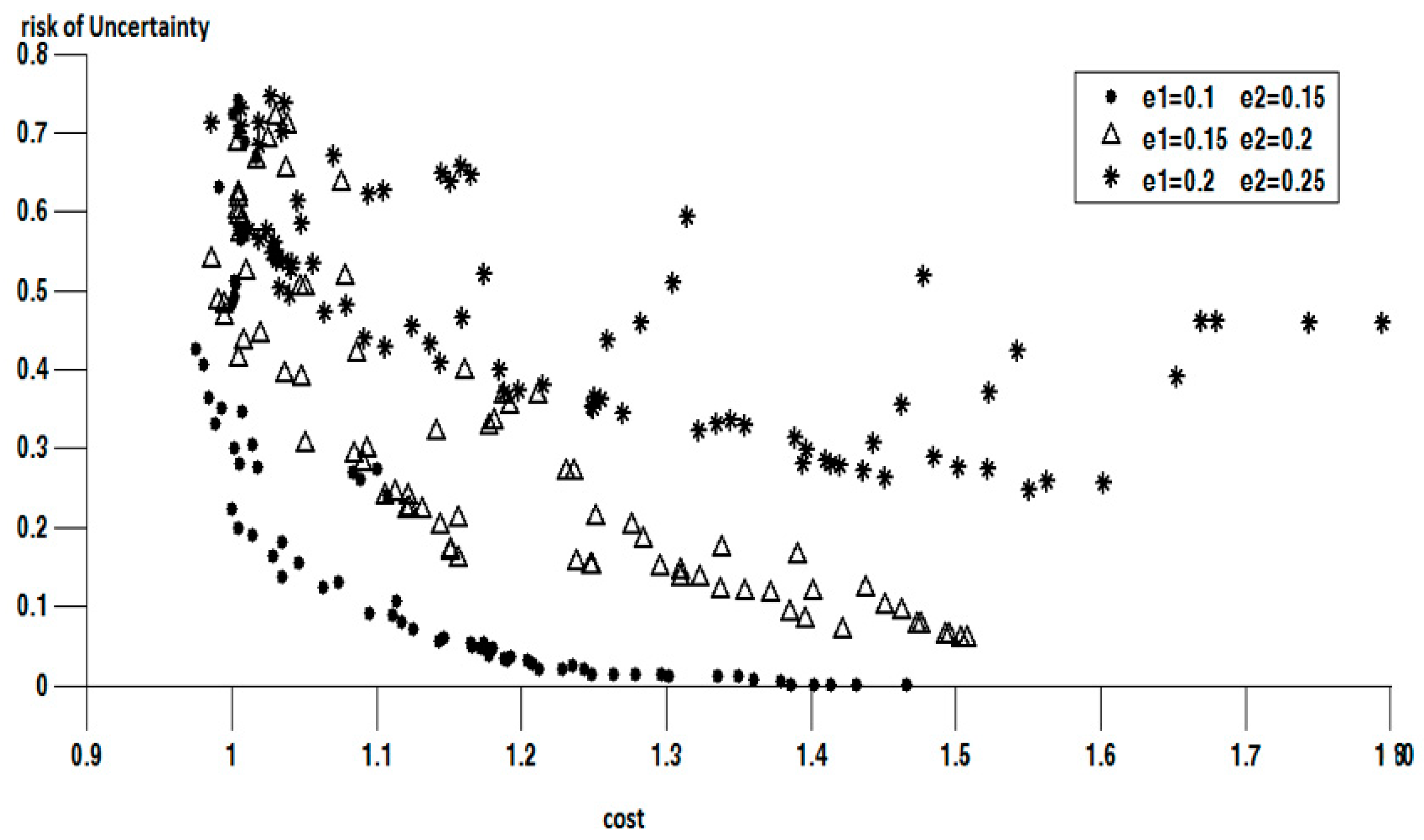
8.2. The Second Experiment

In this experiment, the method of affecting load uncertainty on costs, voltage risk and system instability risk is studied. As mentioned before, the amount of uncertainty in the load varies by changing the uncertainty parameters (e1, e2). In this experiment, by changing these parameters in accordance with

Table 5. Changes in uncertainty parameters.

Experiment No.	Maximum Error e1	Maximum Error e2
1	0.1	0.15
2	0.15	0.20
3	0.20	0.25

, the effect of uncertainty on system costs and voltage risks and instability is investigated.

The rest of the parameters of each experiment are considered according to Table 3. In fact, the first experiment is the same as the previous one, but the second and third tests are performed separately. After performing all the steps mentioned in the previous section for the second and third tests, the results will be obtained as an efficient answer for each experiment. Two-dimensional diagrams of each function have been used to better illustrate the effect of increasing uncertainty on each of the objective functions. In these diagrams, the objective functions are shown in pairs. Figure 11 shows a two-dimensional diagram of the economic objective function and the risk of instability. In this figure, it is clear that with increasing load uncertainty, the economic objective function and voltage risk increase. In fact, the trend of changing charts is such that with increasing uncertainty, the whole chart for each experiment is pushed to the right and up (higher risk of instability and cost).

Figure 12 and Figure 13 show two-dimensional diagrams of other objective functions of these experiments. In these figures, the rate of increase of objective functions is observed following the increase of uncertainty. Another point to note in these figures is that in all three experiments, many of the answers improve the voltage risk by a small amount. This means that voltage risk has better compensability than instability risk.

8.3. Comparing the Proposed Method with Other Capacitor Placement Methods Considering the Fixed Capacitor

One of the methods of validation of the method used is comparison with other articles in the field of project work. After reviewing many articles on capacitance and voltage instability in distribution networks, the articles with the best results were selected for comparison. In these papers, regardless of moment load changes, fixed capacitors were used to improve the stability index as well as reduce losses.

In this analysis, all network nodes except the first bus are considered as candidate locations for capacitors with fixed capacitors. Economic information, uncertainty parameters (e1 and e2) and genetic algorithm parameters are given in Table 3. The load level in this experiment is considered constant and equal to the values of the base load level. After implementing the algorithm to find a Pareto response in the study network, the results are compared with other papers. Figure 14 shows the three-dimensional space of the Pareto answer to this experiment.

In order to examine the answer obtained in comparison with other sources, the concept of non-dominance should be used. In general, one answer dominates another answer, which is dominant to at least one of the goals and not worse than any of the other goals. In other words, suppose all parts of the Pareto Front form a page. Now, if the intended reference response is at the top of this page, the reference answer is defeated. If they intersect with the page, it is part of the Pareto Front, and if it is below the page, the reference answer is dominant.

Table 6. Capacitor placement results in different references.

Instability Risk (%)	Voltage Risk (%)	Economic Objective Function ($)	Constant Capacitor Values	Bus No.	Ref.
57.9	0.83	99,875	1200	6	[29]
			150	8
17.3	0.73	1,116,735	150	18	[30]
			45	17
			75	16
			90	15
			105	14
			180	13
			225	12
			150	32
			150	31
40.58	0.41	105,856	150	13	[31]
			150	14
			150	15
			150	16
			750	30
			150	31
			150	32

shows the results of capacitor placement with fixed capacitor in the studied network.

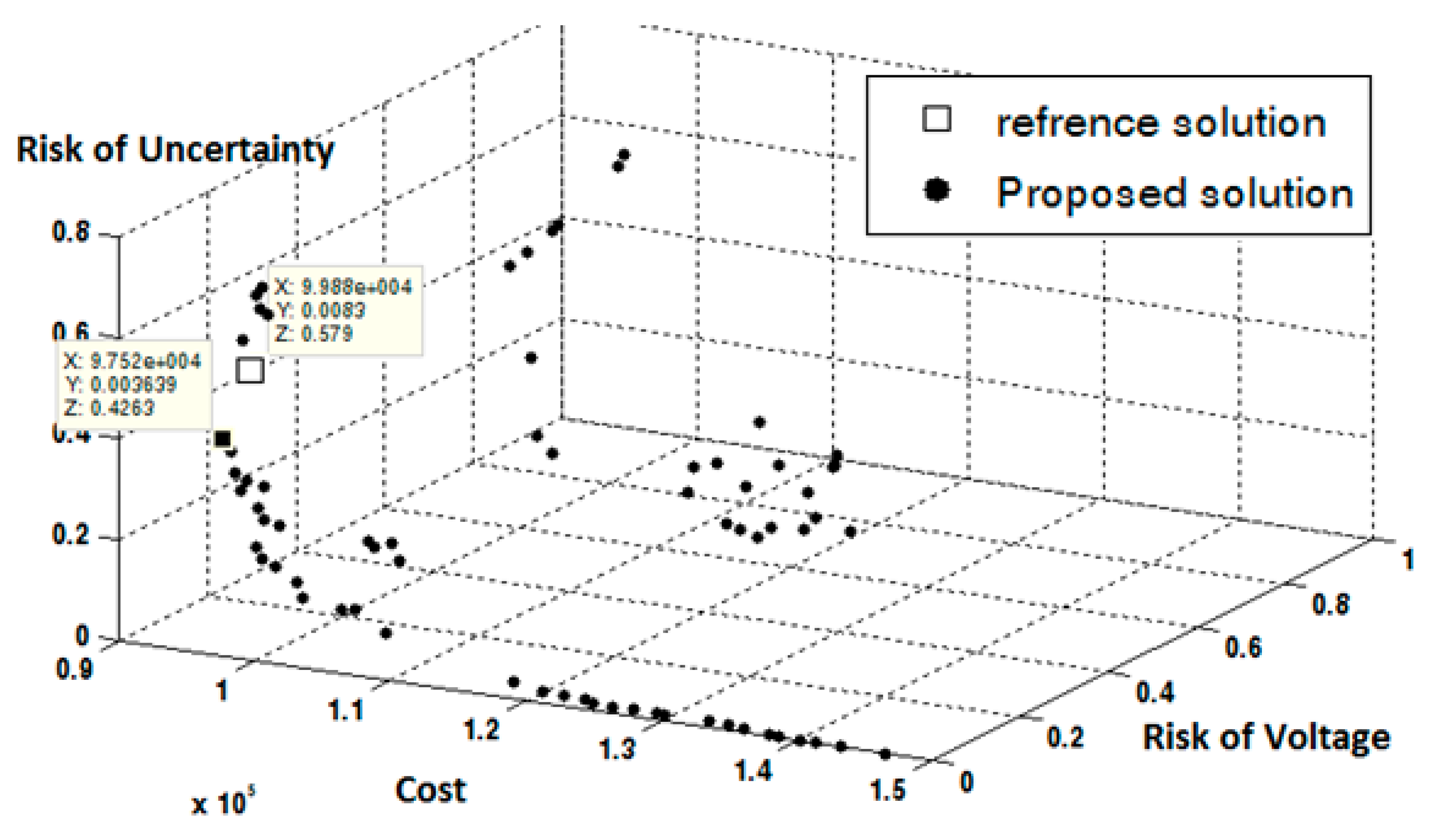
We first examine reference response [29]. The values of the objective functions of this reference are given in Table 6. As mentioned, in light of the proposed Pareto Front of this paper, which is shown in Figure 14, an answer must be found where all its objective functions can dominate the reference objective functions; otherwise the reference response itself is dominated. Figure 15 provides a comparison between the reference responses. A member of the Pareto Front is also identified in this figure. In this figure, it is clear that all objective functions have lower values than the reference objective functions. Therefore, as mentioned, this answer is at the top of the page passing through the members of the Pareto Front and is dominated by the member specified in the figure.

In [31], as can be seen in the figure, the values of the objective function of a member of the Pareto Front were able to dominate [30]. In addition to superiority in the economic objective function, the risk of instability in the Pareto Front member is 5%, and the voltage risk is 0.4% better.

Figure 16, compares answer [30] with the Pareto Front obtained from the location of a fixed capacitor.

Figure 17 also compares answer [31] with that of a Pareto Front member.

In response to answer [31], it is clear that there is a high risk of instability. The values of the objective functions in the Pareto Front response proposed by the project (the point specified in the figure) are less than all the values of the objective functions [31], and according to the concept of non-dominance, it can be said that this answer was also dominated by Pareto Front.

9. Conclusions

The use of fixed and switching capacitors can have significant benefits in reducing energy and power losses as well as improving the stability and voltage profile of the distribution network. However, due to the uncertainty in load data, the location of this equipment is associated with certain complexities so that one of the main problems in analyzing distribution network problems is the lack of sufficient data or the uncertainty in network information in general.

In this paper, we have tried to model uncertainty in load information using the concept of fuzzy numbers. Due to fuzzy load uncertainty modeling, it is necessary to obtain all equations and relations using fuzzy relations. In this regard, the backward–forward sweep load flow was modified based on the mathematical relations of fuzzy numbers.

Exceeding the allowable voltage limits is modeled using risk-based concepts. Risk of instability is one of the new concepts discussed in this paper. First, the stability index in the network containing uncertain information was calculated. Then, the risk of violating the stability index was calculated from the allowable stability limit. Reducing this risk, which is one of the goals of the network, increases the stability of the network.

Reducing the objective functions of instability risk, voltage risk and system costs are the main objectives of this paper, which were achieved using a multi-objective genetic algorithm.

Although the initial investment cost of this type of capacitor is higher, it is reversible due to the profit from reducing network losses over a period of time. In the present paper, by examining the effect of changing the parameters related to uncertainty (e1 and e2) on cost indices, voltage risk and load instability risk, it was observed that the amount of load uncertainty has a significant effect on increasing system costs as well as technical risks including risk of voltage and risk of instability.

The additional suggestions of the paper are presented as follows:

• The behavior of the network in the presence of both definite and non-deterministic information in various issues of the electrical energy distribution system can be investigated.
• The relationship between the uncertainty type of consumption of subscribers or in other words, different tariffs, is an interesting topic that helps in perfecting the way of modeling load uncertainty.
• By installing measuring devices, the amount of uncertainty in load information is reduced. However, installing these devices will increase the cost of the system. Therefore, the economic objective function model can be modified by considering these costs.
• One of the sources of uncertainty in power system studies is distributed generations. The power generation of each of these sources can be simulated with the model presented in this research.
• In the study of restructuring the distribution system, forecasting market information is associated with uncertainty. Using triangular fuzzy numbers can be a good solution for modeling this information.

References

- Mouwafi, M.T.; El-Sehiemy, R.A.; Abou El-Ela, A.A. A two-stage method for optimal placement of distributed generation units and capacitors in distribution systems. Appl. Energy 2022, 307, 118188. [Google Scholar] [CrossRef]
- Kien, L.C.; Nguyen, T.T.; Phan, T.M.; Nguyen, T.T. Maximize the penetration level of photovoltaic systems and shunt capacitors in distribution systems for reducing active power loss and eliminating conventional power source. Sustain. Energy Technol. Assess. 2022, 52, 1–21. [Google Scholar]
- Kasturi, K.; Nayak, C.K.; Patnaik, S.; Nayak, M.R. Strategic integration of photovoltaic, battery energy storage and switchable capacitor for multi-objective optimization of low voltage electricity grid: Assessing grid benefits. Renew. Energy Focus 2022, 41, 104–117. [Google Scholar] [CrossRef]
- Shaik, M.A.; Mareddy, P.L.; Visali, N. Enhancement of Voltage Profile in the Distribution system by Reconfiguring with DG placement using Equilibrium Optimizer. Alex. Eng. J. 2022, 61, 4081–4093. [Google Scholar] [CrossRef]
- Chen, G.; Zhang, J.; Ziabari, M.T. Optimal allocation of capacitor banks in distribution systems using particle swarm optimization algorithm with time-varying acceleration coefficients in the presence of voltage-dependent loads. Aust. J. Electr. Electron. Eng. 2022, 19, 87–100. [Google Scholar] [CrossRef]
- Gampa, S.R.; Das, D. Optimum placement of shunt capacitors in a radial distribution system for substation power factor improvement using fuzzy GA method. Electr. Power Energy Syst. 2016, 77, 314–326. [Google Scholar] [CrossRef]
- Al-Muhanna1, A.A.; Al-Muhaini, M. Reliability impact for optimal placement of power factor correction capacitors considering transient switching events. J. Eng. 2019, 11, 8185–8192. [Google Scholar] [CrossRef]
- Sadeghian, O.; Oshnoei, A.; Kheradmandi, M.; Mohammadi-Ivatloo, B. Optimal placement of multi-period-based switched capacitor in radial distribution systems. Comput. Electr. Eng. 2020, 82, 106549. [Google Scholar] [CrossRef]
- Addisu, M.; Salau, A.O.; Takele, H. Fuzzy logic based optimal placement of voltage regulators and capacitors for distribution systems efficiency improvement. Heliyon 2021, 7, 1–9. [Google Scholar] [CrossRef]
- De Araujoa, L.R.; Penidoa, D.R.R.; Carneiro, S., Jr.; Pereira, J.L.R. Optimal unbalanced capacitor placement in distribution systems forvoltage control and energy losses minimization. Electr. Power Syst. Res. 2018, 154, 110–121. [Google Scholar] [CrossRef]
- Mohkami, H.; Hooshmand, R.; Khodabakhshian, A. Fuzzy optimal placement of capacitors in the presence of nonlinear loads in unbalanced distribution networks using BF-PSO algorithm. Appl. Soft Comput. 2011, 11, 3634–3642. [Google Scholar] [CrossRef]
- Taher, S.A.; Hasani, M.; Karimian, A. A novel method for optimal capacitor placement and sizing in distribution systems with nonlinear loads and DG using GA. Commun. Nonlinear Sci. Numer. Simul. 2011, 16, 851–862. [Google Scholar] [CrossRef]
- Abul’Wafa, A.R. Optimal capacitor placement for enhancing voltage stability in distribution systems using analytical algorithm and Fuzzy-Real Coded GA. Electr. Power Energy Syst. 2014, 55, 246–252. [Google Scholar] [CrossRef]
- Radetz, J. The New IEEE Standard Dictionary of Electrical and Electronic Terms, 5th ed.; IEEE Press: Piscataway, NJ, USA, 1993. [Google Scholar]
- Dai, Y. Framework for Power System Annual Risk Assessment. Ph.D. Dissertation, Iowa State University, Ames, IA, USA, 1999. [Google Scholar]
- Borkowska, B. Probabilistic load flow. IEEE Trans. Power Appar. Syst. 1974, 93, 752–759. [Google Scholar] [CrossRef]
- Brownell, G.; Clark, H. Analysis and solutions for bulk system voltage instability. Comput. Appl. Power 1989, 2, 31–35. [Google Scholar] [CrossRef]
- Haghifam, M.-R.; Falaghi, H.; Malik, O.P. Risk-based distributed generation placement. IET Gener. Transm. Distrib. 2008, 2, 252–260. [Google Scholar] [CrossRef]
- Jasmon, G.; Lee, L. Stability of load flow techniques for distribution system voltage stability analysis. IEE Proc. C Gener. Transm. Distrib. 1991, 4, 479–484. [Google Scholar] [CrossRef]
- Chen, J.-F.; Wang, W.-M. Steady-state stability criteria and uniqueness of load flow solutions for radial distribution systems. Electr. Power Syst. Res. 1993, 28, 81–87. [Google Scholar] [CrossRef]
- Adetokun, B.B.; Ojo, J.O.; Muriithi, C.M. Reactive power-voltage-based voltage instability sensitivity indices for power grid with increasing renewable energy penetration. IEEE Access 2020, 8, 85401–85410. [Google Scholar] [CrossRef]
- Haque, M. Novel method of assessing voltage stability of a power system using stability boundary in P-Q plane. Electr. Power Syst. Res. 2003, 64, 35–40. [Google Scholar] [CrossRef]
- Sajjadi, S.M.; Haghifam, M.-R.; Salehi, J. Simultaneous placement of distributed generation and capacitors in distribution networks considering voltage stability index. Int. J. Electr. Power Energy Syst. 2013, 46, 366–375. [Google Scholar] [CrossRef]
- Jabari, F.; Sanjani, K.; Asadi, S. Optimal Capacitor Placement in Distribution Systems Using a Backward-Forward Sweep Based Load Flow Method. In Optimization of Power System Problems; Studies in Systems, Decision and Control; Pesaran Hajiabbas, M., Mohammadi-Ivatloo, B., Eds.; Springer: Cham, Switzerland, 2020; pp. 63–74. [Google Scholar] [CrossRef]
- El-Hawary, M.E. Electric Power Applications of Fuzzy Systems; Wiley-IEEE Press: New York, NY, USA, 1998. [Google Scholar]
- Lu, J.; Zhang, G.; Ruan, D. Multi-Objective Group Decision Making: Methods, Software and Applications with Fuzzy Set Techniques; Imperial College Press: London, UK, 2007. [Google Scholar]
- Hartono, H.; Azis, M.; Muharni, Y. Optimal capacitor placement for IEEE 118 bus system by using genetic algorithm. In Proceedings of the 2019 2nd International Conference on High Voltage Engineering and Power Systems (ICHVEPS), Denpasar, Indonesia, 1–4 October 2019; pp. 1–5. [Google Scholar]
- Aravindhababu, P.; Mohan, G. Optimal capacitor placement for voltage stability enhancement in distribution systems. ARPN J. Eng. Appl. Sci. 2009, 4, 88–92. [Google Scholar]
- Mohan, G.; Aravindhababu, P. A novel capacitor placement algorithm for voltage stability enhancement in distribution systems. Int. J. Electron. Eng. 2009, 1, 83–87. [Google Scholar]
- Chen, P.; Chen, Z.; Bak-Jensen, B. Probabilistic load flow: A review. In Proceedings of the 2008 Third International Conference on Electric Utility Deregulation and Restructuring and Power Technologies, Nanjing, China, 6–9 April 2008. [Google Scholar]
- Taher, S.A.; Bagherpour, R. A new approach for optimal capacitor placement and sizing in unbalanced distorted distribution systems using hybrid honey bee colony algorithm. Int. J. Electr. Power Energy Syst. 2013, 49, 430–448. [Google Scholar] [CrossRef]
Figure 1.
Graphical representation of the load as a triangular fuzzy number.
Figure 2.
Graphical representation of the voltage of a node as a triangular fuzzy number.
Figure 3.
Single transfer line diagram considering load uncertainty.
Figure 4.
of the fuzzy variables of source voltage, load bus voltage and load power.
Figure 6.
Stability membership function curve.
Figure 7.
Capacitor problem coding method with fixed and switching capacitors.
Figure 8.
The concept of swarm distance for point i.
Figure 9.
Pareto response space in fixed and switching capacitors placement in the distribution network under study.
Figure 10.
Final response capacitance status in the studied network.
Figure 11.
Two-dimensional diagram of economic objective function and instability risk in different experiments.
Figure 12.
Two-dimensional diagram of economic objective function and voltage risk in various experiments.
Figure 13.
Two-dimensional diagram of instability risk and voltage risk in different experiments.
Figure 14.
Pareto response space in locating fixed capacitors in the studied network.
Figure 15.
Comparison of reference [
29] response with the Pareto Front obtained from fixed capacitor placement.
Figure 16.
30] response with the Pareto Front obtained from fixed capacitor placement.
Figure 17.
31] response with the Pareto Front obtained from fixed capacitor placement.