1. Introduction
Images taken directly can only present the information content of part of the band, considering the limitations of imaging equipment. With the image fusion of multi-band key information, a new image containing more information can be reconstructed. High-quality fused infrared and visible images can provide strong complementary information and have high-value applications in many fields, such as target detection, target tracking, automatic driving, and video surveillance. In recent years, image fusion algorithms have gradually developed into two categories: traditional methods and methods based on deep learning. The most typical case based on conventional methods is image fusion methods based on multi-scale transformation, including discrete wavelet transform [
1,
2], non-small downsampling shear wave transform [
3], and so on. Representation-based learning methods are also widely used in this field, such as sparse representation [
4] and joint sparse representation [
5]. Subspace-based, saliency-based, and chaotic model-based methods are applied to image fusion. Nevertheless, traditional methods are not ideal due to problems such as complex design rules and weak generalization ability of scenes.
In the field of image fusion, the rapid development of deep learning is also reflected. The mainstream methods include the convolution network-based method, the codec network-based method, and so on. Deep learning includes mainly three elements: deep feature extraction, fusion strategy, and end-to-end training mode. Specifically, depth feature extraction usually consists of a convolution layer [
6,
7], a designed residual structure [
8], a special feature extraction module [
9], etc. However, the current network’s ability to extract tiny features still needs to be improved. Most networks only transmit the final convolution results to the fusion module, which makes the information of the middle layer lost. Fusion strategies are used to fuse the extracted feature information. Some networks use manual methods to design fusion strategies [
10,
11], while others use deep learning methods to design fusion strategies [
12,
13]. Unlike manually designed fusion strategies, deep learning-based strategies have stronger generalization ability in different scenarios because they can learn from the training data. However, there are still problems such as poor details preservation after fusion and training difficulty for learnable fusion structures.
This paper proposes a new end-to-end fusion framework to address the above problems. A fusion strategy based on convolutional layers is designed, which can follow the network for training. As a result, the depth extraction features can be more effectively utilized, reducing the training difficulty. In addition, in the feature extraction part of the network, a gradient operator feature extractor based on Laplace is designed to replace the work of many convolution layers. An efficient channel attention network (ECANet) is used as the last step of depth feature extraction to reduce the number of network layers and shorten the fusion time. Moreover, aiming at the problem of information loss in the middle layer of feature extraction, this paper adopts the method of feature extraction and feature reconstruction in the network so that different levels of information can be retained in the fused image.
In the aspect of loss function design, this paper designs a combined loss function, which includes strength loss, texture loss, and structure loss. It restricts the retention of pixel intensity features of infrared images, the retention of texture details of visible images by texture loss, and the retention of edge structure features of source images by structure loss.
Finally, the network is verified by comparative experiments on several public infrared and visible fusion data sets, and the corresponding subjective and objective analysis is made. Compared with the comparison algorithm, the fusion results obtained by the proposed method have a better visual effect, and the target definition and background details are more perfect.
3. Detailed Work
In this section, the construction and training methods of the fusion network in this paper will be introduced in detail.
Section 3.1 introduces the main network framework of the method,
Section 3.2 introduces two feature extraction modules, and
Section 3.3 and
Section 3.4 introduce the network’s training method, the setting of super parameters, and the composition of the loss function.
3.1. Converged Network Framework
The method proposed in this paper is an end-to-end network structure, and its composition is shown in
Figure 1. This learning method touts the advantages of synergy and easier global optimal solutions than non-end-to-end networks. The network framework is based on the classical codec network, including the encoder, fusion part, and decoder part. See
Table 1 below for detailed composition.
In this paper, the input infrared image and visible image are defined as and , respectively. In the feature extraction module, the visible light intermediate feature extracted by the Laplace gradient operator extractor (LGOE) layer is , the infrared feature is , and represents the number of feature extraction layers. The fusion result of the output network is , and all the source images of the input network have been registered.
In the encoder part, this paper uses the trained model to multi-level encode the input source image to extract different scale features, including a specific layer of 3 ∗ 3 convolution extraction for extracting rough features, two layers of LGOE, and one layer of the ECA attention module. The encoder network used in this paper has the following three advantages. Firstly, the convolution kernel size is 3 ∗ 3, and the step size is 1, which makes the size of the input image unlimited. Secondly, the use of LGOE can extract depth features and detailed information of images as much as possible to ensure that all salient features are transmitted backward. Thirdly, the channel attention (ECA) module will not increase many parameters and network complexity under improving network performance. The strategy of the above feature extraction module will be introduced in detail below.
In the decoder part, the convolution layer of three 3 ∗ 3 convolution kernels is selected as the decoding part, which is used to reconstruct the fused image. Such a simple but effective structure can express the extracted information well, keep the network low complexity, and avoid too low a fusion efficiency and long training time.
The features and advantages of the fusion network in this paper are introduced in general, and the feature extraction and fusion modules are introduced in detail below.
Laplace-based gradient operator extractor
3.2. Feature Extraction Module
The encoder is usually used for feature extraction in image processing tasks, and this basic feature extraction structure is widely used because of its portability and effectiveness. The encoder in this paper consists of a convolution layer, two LGOE layers, and an ECA attention layer.
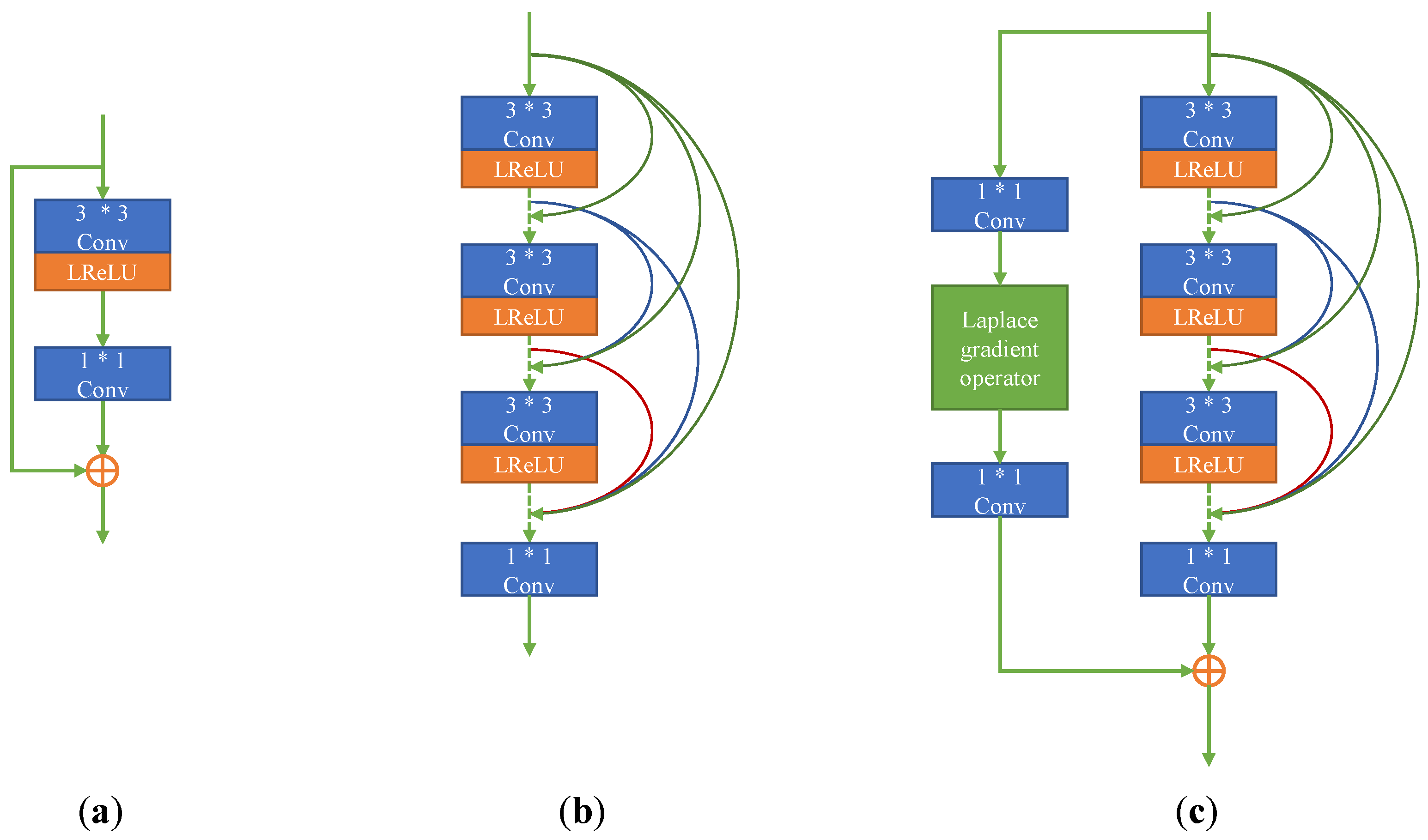
3.2.1. Laplace-Based Gradient Operator Extractor
The basic convolution layer can realize the selection and backward transmission of image features, but some image details will be lost in the transmission process. To enhance the network’s ability to extract fine-grained features from the source image, this paper designs a gradient operator feature extractor based on Laplace. The structure of LGOE is shown in
Figure 2. Each LGOE contains three 3 ∗ 3 convolution layers, with the activation function of Leaky Rectified Linear Unit (LReLU). The dense connection is used in the three-layer convolution to improve the feature extraction ability.
After dense connection, a regular convolution layer with convolution kernel 1 ∗ 1 is added to eliminate the difference in the channel number. In the residual part, a special convolution layer is designed according to the Laplacian gradient operator to extract the fine granularity features of the image. Finally, the extracted depth and fine granularity features are fused and output. LGOE is placed in this paper’s second and third layers of the feature extraction layer.
Aiming at the advanced semantic features in infrared and visible light, this paper proposes a gradient operator feature extractor based on Laplace. Let the image of the input LGOE be
, and its output
can be expressed as follows:
where
represents convolution layer,
represents N cascaded convolution layers, and
represents the summation of elements in tensor.
is a gradient operator, a special convolution operation, and the convolution kernel is the Laplacian convolution kernel. The network can extract fine-grained features by convolution operation between the input features and the high-frequency convolution kernel.
3.2.2. ECAnet
ECAnet [
25] is a new lightweight channel attention mechanism type, as shown in
Figure 3. This structure uses a local cross-channel interaction strategy without dimensionality reduction and a method of adaptively selecting the size of the one-dimensional convolution kernel. The purpose is to ensure the model’s high computational performance and low complexity and achieve noticeable performance improvement with a few additional parameters.
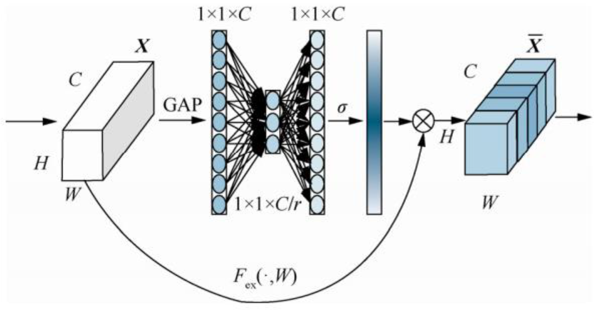
ECANet is improved based on SENet [
23]. This network is a new image model proposed in 2017 that can improve network performance by modeling the correlation between feature channels, called the channel attention mechanism. SENet consists of compression, excitation, and feature recalibration, and the network mechanism is shown in
Figure 4. Compared with SENet, ECANet uses fewer parameters and avoids the negative impact of dimensionality reduction. The structure of ECANet is shown in
Figure 3. The main difference between ECANet and SENet is that the former omits the step of dimensionality reduction after GAP. Instead, it uses the channel and its adjacent K channels to obtain cross-channel communication information.
Let the dimension of the output of a convolutional layer layer be
, where W, H, and C represent the width, height of tensor, and the number of convolution kernels, respectively. The weight of each channel in the SENet network is calculated as follows:
where
is global average pooling (GAP),
is Sigmoid function.
has the following relationship with:
ReLU stands for the rectified linear unit , but this processing method destroys the direct relationship between channel and weight.
In ECANet, dimension reduction is not required for
after GAP, so
where
is the parameter matrix of
. In ECANet,
it is used to indicate the learned channel attention:
includes
parameters, and only
and its k adjacent information interactions are considered for the weight
:
where
represents the set of k adjacent channels o
. Afterward, all channel weight information is shared to improve performance:
To sum up, this method realizes the information interaction between channels through one-dimensional convolution with convolution kernel size
k:
where CID represents one-dimensional convolution, which contains k parameter information. This ability of cross-channel information interaction ensures the performance and efficiency of the network. The value of
k is determined in the subsequent experiment.
3.3. Fusion Structure
In the fusion network based on deep learning, most authors choose simple manual strategies for deep feature fusion [
6,
26,
27], such as elementwise-add, elementwise-mean, elementwise-maximum, and elementwise-sum. Moreover, this fusion method only focuses on deep convolution features, ignoring the importance of shallow features in the fusion network. To solve this problem, this paper uses a network structure based on a convolution layer to fuse deep features and uses the rule for the highest pixel value to fuse shallow features.
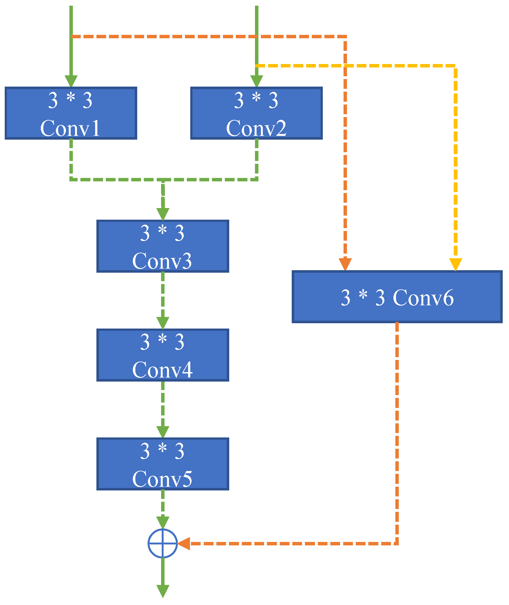
The Central fusion network (CFN) used in this paper is a variant of a simple convolution module used in the fusion of deep image features. Its structure is shown in
Figure 5. In this network, “Conv1”, “Conv2,” and “Conv6” are the first layer of fusion features. “Conv1” and “Conv2” are connected in series as the input of “Conv3”, and “Conv6” is input as the residual.
The structure of CFN is simple and light, so it will not produce too many parameters, and the training difficulty is low. It can be seen from the comparative experiments that CFN has a better effect than other methods commonly used in fusion.
For the fusion of shallow features, the convolution results of the previous part of the encoder are fused and transmitted to the decoder to realize the preservation of shallow features in the fused image. Since each pixel value of the convolved feature map can represent a certain area of the original image and has a high information value, this paper selects the maximum pixel value.
3.4. Loss Function
In the network training stage, we need to train the feature extraction ability of the coding layer and the feature reconstruction ability of the decoding layer at the same time.
Ground truth plays a crucial role in traditional CNN network training, and it is usually used to test the accuracy of the training set’s classification of supervised learning techniques. However, the result of the image fusion network in this paper is a fusion image that includes both infrared target information and visible light details, so there is no Ground truth. This paper designs a combined loss function for such a special case to guide the network’s training. A loss function is generated by an appropriate combination strategy to minimize the loss of network training.
The loss function in this paper consists of three parts: strength loss, texture loss, and structure loss. The total loss is as follows:
where
represents strength loss, which restricts the pixel performance of the fusion result, mainly aiming at the target features of infrared images.
indicates texture loss, which restricts the embodiment of the detailed information of the fusion result, mainly aiming at the fine-grained background information of visible light images.
and
is the weight used to balance the losses. The value of
is set to 10 according to the research and
is set to 0.5 after the research in this paper. For the specific analysis experiment, see the parameter verification section in the chapter on experimental verification. The formula of
is as follows:
where
represent the height and width of the image, respectively,
represents the L1 norm, and
means that the maximum value is selected pixel by pixel. The formula of
is as follows:
SSIM [
28] is a typical image evaluation algorithm representing the structural similarity between the standard image and the image to be evaluated. In this paper, SSIM is used to constrain the overall structure of the fused image. If the marked image is
, the image to be evaluated is
, the input infrared image is
, and the visible input image is
, then the formula of
is as follows:
where
indicates the average value of pixels of image
and image
,
represents the covariance between image
and image
,
are constant, set to 0.2 based on a previous experiment [
29].
are the height and width of the image, respectively, and
is used to balance the weights of the respective structural similarities between the infrared and visible images.
4. Experimental Verification
4.1. Experimental Environment and Data Preparation
The experimental environment of this paper is as follows: Intel (R) Core (TM) i9-9820X processor, NVIDIA GeForce RTX 3090 GPU, win11 operating system, software environment pytorch 3.6 (Pytorch.org, Warsaw, Poland), network training software platform pycharm, and test algorithm platform matlab2021b (The MathWorks, Inc., Natick, MA, USA).
For the selection of data sets, this paper chooses the RoadScene data set as the training set and test set of this network model, and the TNO data set and some RoadScene data sets as the verification set. One thousand pairs of infrared and visible images in the data set are selected for network training, and 360 pairs of infrared and visible images in the data set are selected as test sets. All the images in the data set have been registered so that this paper can import the data directly into the network. In this paper, the learning rate is set to decline with the number of rounds during training, the initial learning rate is 0.001, and the learning rate decreases by 25% for each round of training. Adam solver is used to optimizing the loss function, and the size of each round is set to 8, and a total of 30 rounds are trained.
For the selection of evaluation indicators, this paper selects a group of commonly used performance evaluation indicators of Fusion I. The index system is mainly divided into four categories, which are evaluation indicators based on information theory, including EN (entropy) [
30], MI (mutual information) [
31], and PSNR (peak signal to noise ratio) [
32]. MSE (mean-square error) based on structural similarity, SF (spatial frequency) [
33], SD (standard deviation) [
34], AG (Average Gradient) [
35] based on image features, Evaluation index VIF (Visual fidelity) [
36] based on human visual perception, and evaluation index based on source image and generated image, mainly including CC (Correlation Coefficient) [
37], SCD (Difference Correlation) [
38] and Qabf (Gradient-based Fusion Performance) [
39]. To ensure the accuracy and consistency of objective evaluation, all comparative experiments are used in this paper.
4.2. Comparative Experiment
4.2.1. Comparison of Loss Function Parameters
There are two self-defined parameters
in the loss function, and the parameters in the loss function control the proportion of different parts of the combined loss function. In this paper, the parameter
is set to 10, according to the paper [
40]. To evaluate the optimal value of
, the value of
(of this paper is verified by experiments with control variables. Other factors being the same, assign
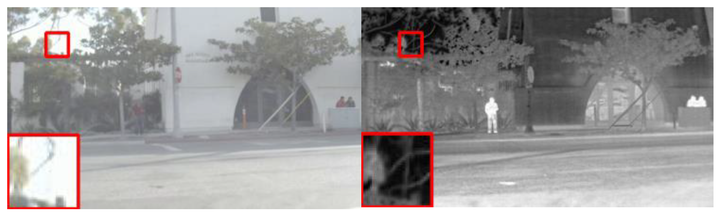
values to 0, 0.1, 0.5, 1, 10, and 100, and conduct network training and testing, respectively. The test uses image pairs in the TNO data set, as shown in
Figure 6.
Figure 7 shows the output results of images with different
values. Intuitively, as the value increases, the result’s overall brightness is gradually improved. When
, it can be seen from the “glass door” part of the picture that visible light information is reflected more, while the “glass door” part of the picture only reflects infrared features when
. It can be preliminarily considered that with the increase of the
value, the fusion results will gradually eliminate the visible light features and retain more infrared features. When
, the infrared features in the red box disappeared, the visible light information of the upper body of the infrared target figure in the picture was erased, so the fusion effect was poor.
Table 2 shows the comparison of objective indicators of experimental results, Objectively speaking, the optimal values of evaluation indexes are scattered, but when
, more indexes reach the highest or second highest point. Based on intuitive and objective comparisons, this paper sets
as the value of the loss function.
4.2.2. Comparison of Convergence Strategies
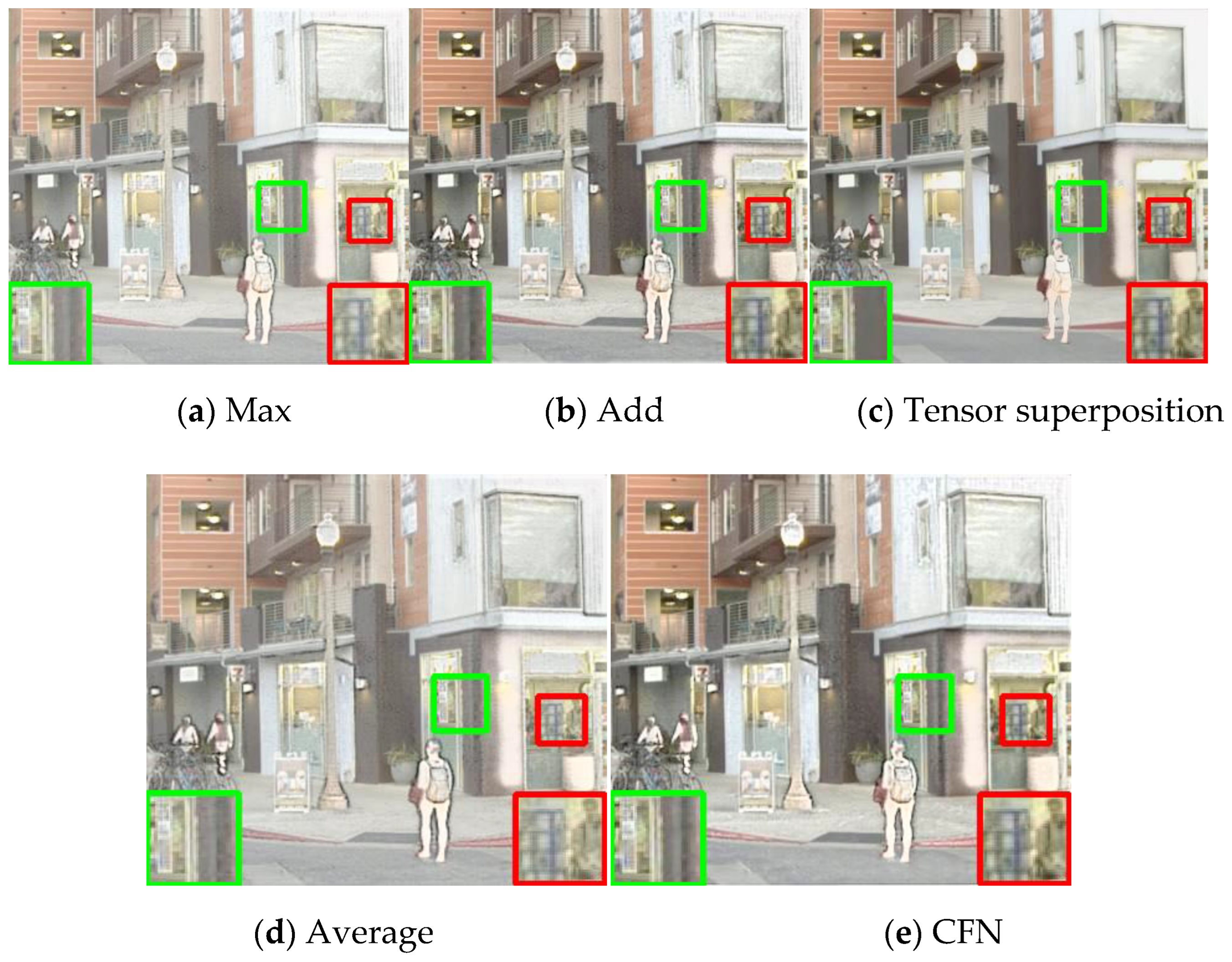
This paper designs a fusion module based on a convolution layer. To verify the superiority of this module over other fusion modules, several commonly used fusion rules are selected, including four methods: maximum selection, tensor dimension superposition, tensor value superposition, weighted average, and a comparative experiment is carried out. In the experiment, an image in the RoadScene dataset is selected as the comparison object, as shown in
Figure 8.
Figure 9 shows the fusion results of replaci ng different fusion modules while keeping other parts consistent. The contrast of the maximum selection method is lower than that of this method, and the overall fusion result has higher brightness and lower contrast. Compared with the method proposed in this paper, numerical addition and tensor dimension superposition erase more infrared details, and the method of tensor dimension superposition looks smoother in the image. The black strip features of the wall with the green box are entirely lost in the results of this method. The results of the weighted average method have some disadvantages, such as low contrast and unclear infrared features.
From the comparison of indexes, several methods can get the best among different indexes, but the method in this paper can get more optimal values, as shown in
Table 3. Combining subjective and objective results, the CFN fusion module proposed in this paper is superior to the contrast method, the fusion results have high contrast, and the infrared and visible features are well reflected.
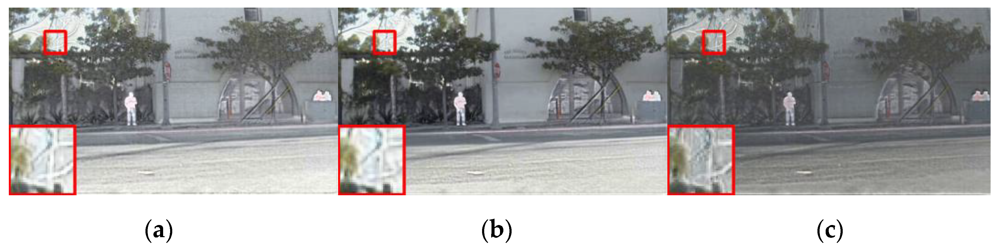
4.2.3. Comparison of LGOE Cascade
This paper uses a two-layer LGOE feature extractor in the encoder for deep feature extraction. To verify whether the number of cascaded layers is optimal, a comparative verification experiment of the LGOE cascade is designed. Under the same other factors, the number of cascaded layers is set to 1, 2, 3, and 4. In the experiment of the 4-level cascade, because the network depth is too deep, it can’t converge at the initial stage of training, and the gradient disappears, so it is possible to exclude 4-level and above as the optimal one. Select an image in the experimental RoadScene data set as the contrast object, as shown in
Figure 10.
Figure 11 shows the fusion results of a different number of feature extractors. Intuitively, with the number of cascades increasing, the brightness of the fusion results gradually decreases. That is, the proportion of infrared images in the fusion results gradually increases; The brightness of the picture is high, but the contrast is low; The brightness of the image is dark, and the infrared target features are not prominent; The overall effect of the picture is good, the clarity and brightness are balanced, the infrared target is prominent, and the visible light details are clear.
From the comparison of objective indicators in
Table 4, when the number of cascades is 2, the evaluation indicators of the fusion effect have obtained the optimal values of most indicators. Compared with other cascades, the fusion results have better performance in objective indicators and intuitive performance. Therefore, two LGOE feature extractors are selected in this paper.
4.3. Fusion Effect Comparison
To prove the effectiveness and superiority of the network architecture proposed in this paper, six fusion algorithms are selected for comparative experiments, namely, Cross Bilateral Filter (CBF) [
41], convolutional neural network (CNN) [
42], Proportional Maintenance of Gradient and Intensity (PMGI) [
43], FusionGAN [
12], IFCNN [
29], U2Fuison [
44].
CBF is an image fusion algorithm based on cross bilateral filter, which is a classical algorithm of traditional image fusion; PMGI is a general image fusion algorithm based on gradient and intensity ratio, which is the same end-to-end deep learning algorithm as this paper, but the main extracted information is pixel gradient and intensity; CNN method uses the same method of convolution to extract features as this paper, but mainly for multi-focused FusionGAN is a fusion algorithm based on GAN algorithm, the basic principle is to generate the image with infrared features and multi-layer visible gradient by generator, and force the fused image to have more visible texture by discriminator, which is the same end-to-end fusion method as this paper, but is a derivative of GAN algorithm; IFCNN is a convolutional neural network based IFCNN is a general image fusion algorithm based on convolutional neural network, which is a more basic fusion method, only extracting the features of the source image through two convolutional layers and passing them into the fusion layer (including three optional methods of element maximum, element minimum or element average) for fusion, which extracts fewer features compared with this paper; U2Fuison is an unsupervised image fusion algorithm, using pre-trained VGG-16 as the feature extractor, and the other parts are based on DenceNet.
To prove the generalization ability of the algorithm, this paper verifies it on the following two data sets.
4.3.1. Comparison of Effects in TNO Data Set
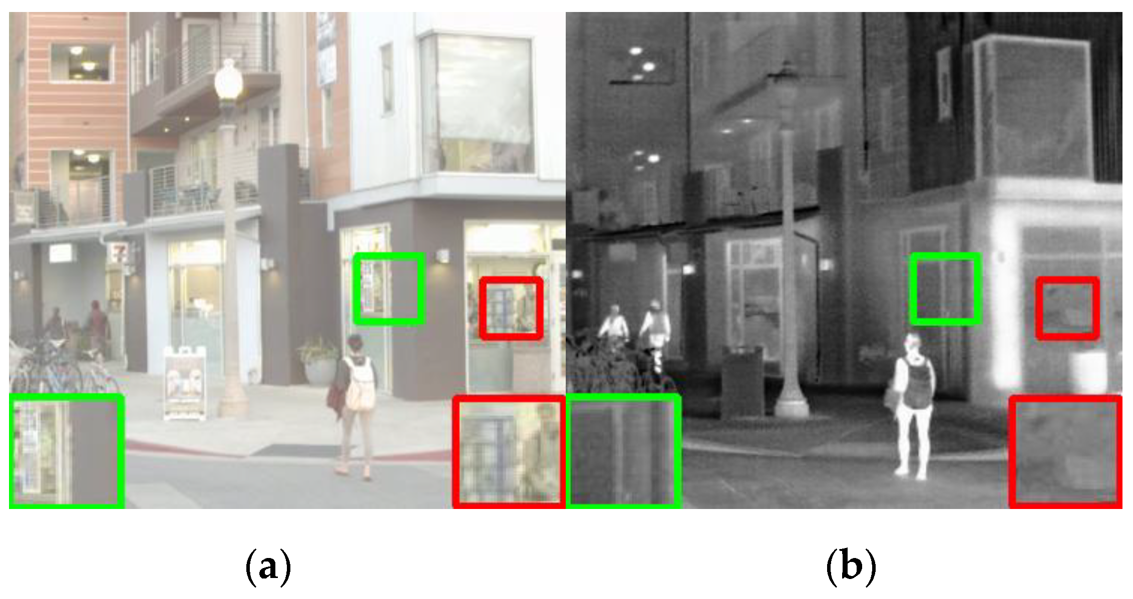
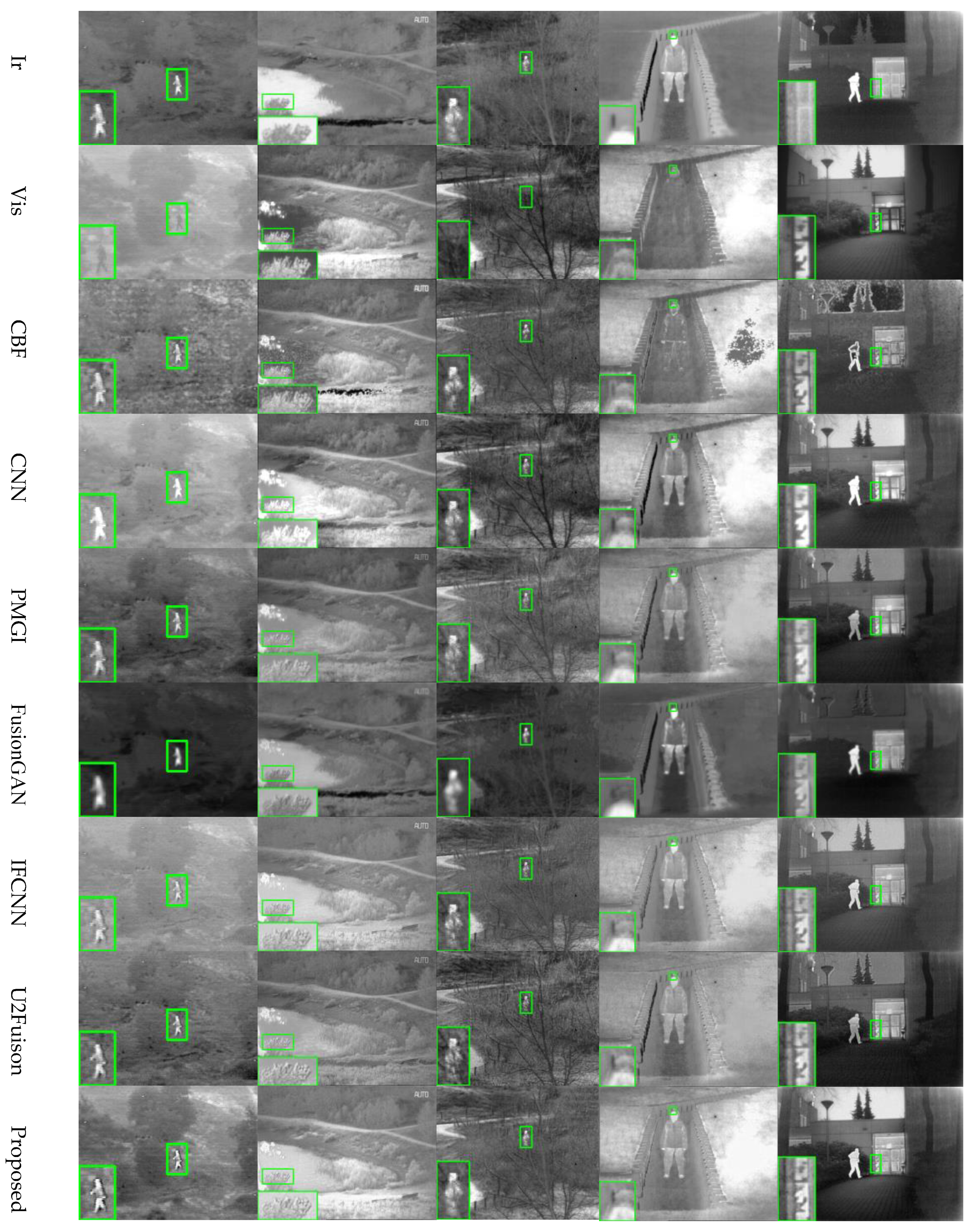
To avoid the chance of data, 36 images in the TNO data set are selected as the source image data of the effect comparison experiment, as shown in the figure. At the same time, five images were selected from the used data for display to visually compare the fusion results of different algorithms without occupying too much space. Some details or main objects in the images were marked and enlarged with green highlighted boxes, and the visible and infrared images as input were placed in the first and second rows. The following are the fusion results obtained by different methods, as shown in
Figure 12.
From an intuitive qualitative point of view, there are obvious gaps in the fusion results of the seven methods. It can be seen that the fusion results of different methods have different emphases. The fusion result of CBF has a poor visual effect and contains a lot of noises that do not exist (for example, the land in the first image, the noise on the right side in the fourth image, and the target outline in the fifth image), and the detailed information is seriously distorted. The results are similar to those of CNN IFCNN, and the overall visual effect is good. However, the contrast of environmental information in the first image is too low, and the fusion effect of the algorithm on low-quality images is poor. The brightness of grass in the enlarged part of the second image is too high, but there is no infrared feature in the source image. The trench’s low brightness feature on the left side in the fourth image completely covers the visible light information.
PMGI U2Fuison has good fusion ability for low-quality source images. The first image has high contrast and full environmental information. In the fifth image, the outline in the glass is unclear, the contrast is low, the overall fusion effect is general, and the sky is gray, so the fusion effect is general. And the visible light information of PMGI in the third image is saved less, which makes fused images less sharp. The overall effect of FusionGAN is poor, and the details are insufficient. For example, the infrared target in the first picture and the infrared target in the fifth picture is not clear in outline, the fusion result is gray, and the contrast is insufficient. Compared with the shortcomings of other methods mentioned above, this paper can achieve a better balance in different quality images, keep clear visible light information in all images, and keep the infrared target bright. The first image has a good fusion contrast, keeping high contrast information, and the second image keeps different brightness for different places, which has a better visual effect based on inheriting the source image information.
The objective evaluation results of indicators are shown in
Table 5, with the best results in red font and the second-best in blue font. From the results, the algorithm proposed in this paper has better performance in this data set, and the fusion results can obtain the optimal and suboptimal values of most indexes.
Specifically, the fusion results of this algorithm have relatively good information entropy, spatial frequency, standard deviation, mean square error, good gradient characteristics in peak signal-to-noise ratio, mutual information, and visual fidelity. Experimental results show that the proposed algorithm has better fidelity, lower distortion, and artifacts in the TNO data set than the comparison algorithm and has a better fusion effect in general.
4.3.2. Comparison of Effects in RoadScene Data Set
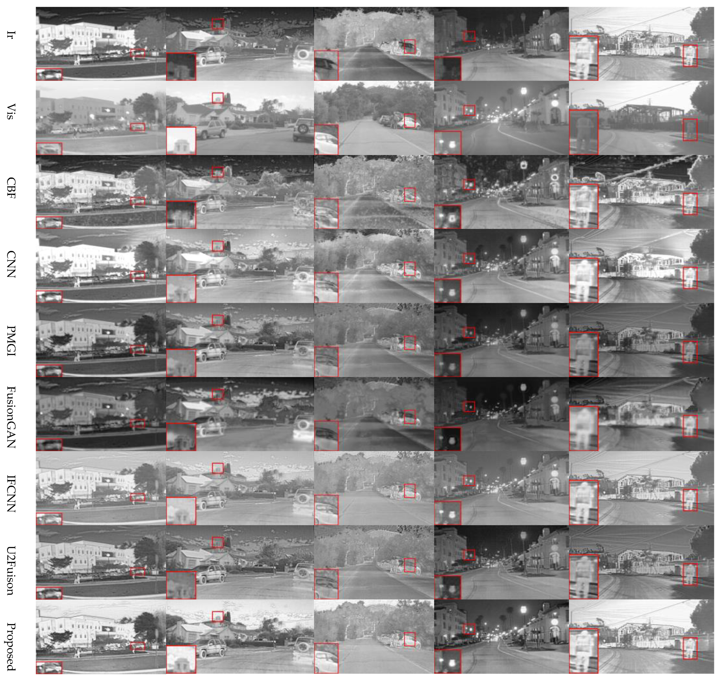
This section tests six comparison algorithms and our algorithm on the RoadScene dataset. The test set is 50 pairs of visible and infrared images selected from the RoadScene data set. Five typical scenes are selected from the results shown in
Figure 13, with local details selected by red boxes and enlarged.
In the figure, the infrared image mainly includes the highlighted thermal radiation infrared information, including pedestrians, vehicles, some buildings, etc. The visible image contains a lot of detailed environmental information. From an intuitive point of view, this method is more prominent in infrared target information retention, and the brightness of people’s vehicles is significantly higher than that of the environment, which is convenient for human eye recognition and subsequent programmed processing. In terms of visible light detail information retention, the overall result details and textures are more clear, and the brightness intensity distribution is appropriate.
Objective Contrast In this paper, 11 evaluation indexes, such as EN, SF, SD, etc., used above are used. After fusing 50 images in the test set, each image is evaluated separately, and the average value is obtained. The best image is marked with red and the second-best is marked with blue. The results are shown in
Table 6. In this paper, the algorithm achieves the best value in spatial frequency, standard deviation, mean square error, average gradient, and difference correlation index, and the second-best value in mutual information, visual fidelity, and gradient-based fusion performance.
Overall, in the test results on the RoadScene data set, compared with other methods, this paper has better information retention ability and better visual effect.


