Framing Network Flow for Anomaly Detection Using Image Recognition and Federated Learning

Abstract

The intrusion detection system (IDS) must be able to handle the increase in attack volume, increasing Internet traffic, and accelerating detection speeds. Network flow feature (NTF) records are the input of flow-based IDSs that are used to determine whether network traffic is normal or malicious in order to avoid IDS from difficult and time-consuming packet content inspection processing since only flow records are examined. To reduce computational power and training time, this paper proposes a novel pre-processing method merging a specific amount of NTF records into frames, and frame transformation into images. Federated learning (FL) enables multiple users to share the learned models while maintaining the privacy of their training data. This research suggests federated transfer learning and federated learning methods for NIDS employing deep learning for image classification and conducting tests on the BOUN DDoS dataset to address the issue of training data privacy. Our experimental results indicate that the proposed Federated transfer learning (FTL) and FL methods for training do not require data centralization and preserve participant data privacy while achieving acceptable accuracy in DDoS attack identification: FTL (92.99%) and FL (88.42%) in comparison with Traditional transfer learning (93.95%).

1. Introduction

A series of operations known as intrusion are intended to compromise the security of computer and network components. Network intrusion detection system (NIDS) offers well-established methods that collect and analyze data from various places within a network to discover potential security breaches in order to protect the network infrastructure [1]. By analyzing current network behaviour patterns or rules, traditional NIDS often assess whether the network connection is in a normal state or not. However, as the Internet is a complex, constantly evolving system, it gathers a tremendous amount of complicated and high-dimensional data. It comes as no surprise that NIDS must be able to handle the increasing attack volume, the expansion of Internet traffic, and the accelerating detection speeds. Conventional NIDS methods have become inadequate as a result [2]. In [3], the challenges of intrusion detection systems (IDSs) are summarized as follows: false alarm rate, low detection rate, unbalanced datasets, and response time.

Deep packet inspection or stateful protocol analysis are traditional methods used by IDS to identify attacks in network traffic. Deep packet inspection is too expensive to be used in terms of processing and energy consumption since real-time classification requires the analysis of a massive volume of data. NIDSs based on flow analysis provide good options for real-time traffic classification as flow-based techniques can categorize the entire traffic by inspecting an equivalent of 0.1% of the total volume [4]. Network flow records are the input of flow-based IDSs, which are used to determine whether network traffic is normal or malicious in order to protect IDS from difficult and time-consuming packet content inspection processing since only flow records are examined [5]. An internet protocol (IP) flow is a collection of packets that are seen in a network over a period of time and have a common characteristic known as its key. These packets can be part of a TCP connection or a UDP stream, and their source and destination IP addresses, source and destination port numbers, protocol numbers, etc., can identify them. There are infinite aggregation strategies in which statistic network packets are collected based on a predefined flow identifier [6].

The Cisco Annual Internet Report [7] shows that both the total number of records exposed and the number of breaches are increasing. When multiple systems overload the bandwidth or resources of a targeted system—typically one or more web servers—it is called a Distributed-Denial-of-Service (DDoS) attack and is the main threat that most service providers have noticed. Attacks between 100 Gbps and 400 Gbps increased by 776% globally between 2018 and 2019, and the total number of DDoS attacks will double from 7.9 million in 2018 to 15.4 million by 2023. NIDS must be constantly improved to avoid malicious activity before it occurs as attackers always come up with new ways to exploit the network [8]. The authors in [9] highlight the research challenges in the field of IDS as follows: (i) systematic construction of an up-to-date dataset with enough instances of almost all the attack types; (ii) lower detection accuracy due to the imbalance dataset; (iii) low performance in a real-world environment; (iv) most of the IDS approaches suggested by the researcher are based on extremely sophisticated models requiring a lot of processing time and computing power. Finally, as stated in [9], one of the main problems is creating a lightweight IDS model that is effective in terms of computational power and training time and has a higher intrusion detection rate.

The idea behind FL is to facilitate the building of a model based on a distributed data set across multiple devices while preventing data leakage. Given data owners, {N₁…N_i}, who wish to build a strong model by consolidating their data (D₁…D_i), conventionally train the model by combining the data, D = (D₁∪…∪ D_i). However, in the FL concept, the owner collaboratively trains the model in such a way that any data owner N_i does not reveal its data D_i to others. Only a subset of the data D_k ⊆ D with N_k samples is used by the k-th party, where k ∈ [1, k]. We assumed that the data points in D allocated to any distinct parties N₁…N_k are disjoint, that is, D₁…D_k are partitions of D. Let matrix D_i define the data held by owner i with each row in the matrix representing a sample. Let F, Y, and J denote the feature, label, and sample ID space, respectively. The training dataset is thus constituted as (F, Y, J) based on how the data are distributed among the subsets, the feature and sample ID space, and FL can be classified as horizontal FL, vertical FL, and federated transfer learning (FTL). In horizontal FL, the data sets have the same feature space but different samples, while in the vertical scenario the datasets have the same sample ID but share different feature space.

Our novelty and the main idea is to use the network traffic feature (NTF) records framing technique to reduce computational power and training time while preserving data privacy using the federated learning (FL) method and the trained models sharing approach.

The main contributions of this paper are:

• Reduced computational power and training time. Overall, 96 times fewer images are required for deep neural network (DNN) training while adopting the proposed pre-processing method merging a specific amount of NTF records into frames and transforming frames into images;
• Preserved data privacy. To ensure data privacy, the FL method was used to share trained models between participants without the need to publicly centralize training data in a data centre. As an example of trained model sharing, GitHub may be used as a distributed version control system, which implies that every developer’s computer has access to the whole codebase and history, therefore making branching and merging simple;
• The detailed experimental analysis. Experiments of the proposed approach presented in three use cases for the DNN training on the classification of DDoS network attack type: (i) traditional transfer learning (TL) method with mandatory training data centralization, (ii) federated transfer learning (FTL) method when participants share only trained models to continue training, (iii) federated learning (FL) method when trained models aggregated in a data centre to create the Global Model for sharing;
• Empirical quantification. In the presented experimental use cases, the testing accuracy of Global Models is strong, ranging from 88.42 per cent to 93.95 per cent. Although the majority class in our instance is normal traffic, the fundamental challenge of identifying normal traffic is being resolved. In our experimental results, high F1 score values of Global Models testing from 93.78% to 96.86% were obtained.

The structure of the remaining parts of the paper is as follows. Section 2 discusses related works. Section 3 presents the methodology. Section 4 presents the results of the experiments. Finally, Section 5 is dedicated to the discussion of the results.

2. Related Works

NIDS can be classified according to their placement in the network, the detection concept, and the response to intrusion or attack [10]. Signature-based detection systems, for example, cannot report deviations that are not in their database as indicative of the network deviation from the norm. At the same time, behavioural systems (anomaly-based), which employ the investigated network’s behaviour—assumed as normal, as an indication—are more likely to have frequent false positives than signature-based systems. In general, signature systems search for established signals of dangerous behaviour in traffic flow, whereas behavioural systems strive to track unusual traffic flow signs. It should be mentioned that researchers are currently concentrating their efforts in the field of behavioural systems based on anomalies (anomaly-based intrusion detection), which are capable of detecting both known and unknown abnormalities. If network intrusions are correctly reflected in the form of an attack, intrusion detection helps to identify them. In this context, an attack pattern is defined as a specific collection of explicitly documented actions related to the assault, the application of which to the fields of the object being identified provides for an unambiguous answer regarding the object’s membership to this attack. In the network anomaly detection scheme, for the detection of network intrusion, the primary data for analysis are network traffic [11]. The highlighted network packet properties are provided to the module, which examines and checks the conformity of input data with the rules and alerts about the presence of danger. The important issue in identifying abuse is the appropriate design of the mechanism for setting the correct intrusion detection. In fact, creating a complete rule base for recognizing all conceivable attacks is impractical, since describing variances in attacking activities might have a negative impact on their performance. Even little changes in the attack make detection impossible; hence, the stated criteria should be general and include more known alterations of network attacks. Although NIDS technologies are useful for recognizing known forms of attacks, their application to novel (zero-day) attacks is limited [12].

Modern ML theory and practice include both conventional areas such as supervised learning and unsupervised learning [13], as well as novel areas such as deep learning [14], reinforcement learning [15], and transfer learning [16]. However, until recently, ML avoided information security concerns throughout the training and application stages of the model. The fact that the majority of ML applications have been local or client/server applications explains the lack of attention to information security problems. To create predictions such as recognition of a class of data, traditional ML employs a data pipeline that uses a central server (on-premises or in the cloud) that hosts the trained model. The disadvantage of this design is that all data collected by local devices and sensors are routed to a central server for processing before being delivered to the devices. The model’s capacity to learn in real-time is hampered by this round-trip.

FL is a technique that trains an algorithm on multiple decentralized peripherals or servers containing local data samples without sharing them. This approach differs from traditional centralized ML methods, where all local datasets are loaded onto a single server, as well as more classic decentralized approaches, which often assume local data samples are equally distributed. The benefits of FL are as follows [16,17,18]:

• FL allows devices, such as mobile phones, to share a common prediction model by keeping training data on the device rather than downloading and storing the data on a central server;
• It shifts model training to the peripheral, namely to devices like smartphones, tablets, the Internet of Things, or even “organizations” like hospitals that must function under strict secrecy constraints. Keeping personal data in situ provides significant security benefits;
• Since forecasting occurs on the device itself, real-time forecasting is feasible. FL decreases the time lag that occurs when raw data is transferred back to a central server and the results are sent to the device;
• As the models are stored on the device, the forecasting process may continue even if there is no Internet connection;
• FL decreases the amount of hardware infrastructure required. FL makes use of minimum hardware, and what is available on mobile devices is more than sufficient to operate the FL models.

Successful examples of FL applications include autonomous vehicles [19], healthcare systems [20], smart cities [21], the Internet of Things [22], industrial manufacturing in Industry 4.0 [23], and others [24]. The maintenance of data privacy is the main benefit of FL here for each participating entity in achieving a common goal [1]. Federated database systems [25], and federated cloud [26] are all examples of federal systems.

Previous research [27] used the KDD’99 dataset and the UNSW-NB15 dataset to describe experiments for intrusion detection in a federated context. FL is coupled with blockchain technology [28] to avoid harmful cyber-attacks. The tests presented here were carried out using supervised autoencoder (SAE) models for anomaly detection in a genuine intrusion detection use case (AWID dataset). They show that adding blockchain has only little influence on FL performance. The authors of [29] present a blockchain-enabled Federated Forest Software Defined Network (SDN) IDS that allows the training of IDS models that facilitate the detection of controller area network (CAN) intrusions into vehicle systems while keeping sensitive data confidential. To construct a random forest model, they employed FL, while the evaluation was performed on the CAN-intrusion dataset (OTIDS). The authors [30] demonstrate that the suggested wireless NID approach is effective in terms of classification accuracy, computation cost, and communication cost in a series of experiments using the AWID intrusion detection dataset. In [31], Huong et al. offer LocKedge—a multi-attack detection method with low complexity for deployment at the edge zone while retaining high accuracy. To test the performance of the architecture from many viewpoints, LocKedge is deployed in two ways: centralized and FL. Using the BoT-IoT data set, the method can detect 10 types of attacks. Li et al. [32] proposed a distributed NIDS using FL in satellite-terrestrial integrated networks (STINs) to properly allocate resources in each domain to analyze and block malicious traffic, including nine attack scenarios such as botnets, web attacks, backdoors, and six different DDoS attacks (LDAP, MSSQL, NetBIOS, Portmap, Syn, UDP). Nguyen et al. [33] proposed to employ an FL approach to anomaly-detection-based intrusion detection in Internet-of-Things (IoT) devices. Qin et al. [34] used binarized neural networks (BNNs) that can be implemented as switch functions at the network edge classifying incoming packets in the context of an FL. Data privacy security guaranteed NIDS based on federated learning proposed in [35]. Tian et al. [36] proposed a specific neural network called a lightweight residual network (LwResnet) using FL architecture for the detection and classification of DDoS attacks. Xie et al. [37] presented an enhanced k-means clustering intrusion detection technique based on FL. To enhance k-means clustering, this approach was coupled with three-way decision concepts and introduced multiple viewpoints of cosine distance as a measure of similarity between data items. Rahman et al. [38] propose the FL-based scheme for IoT intrusion detection that maintains data privacy by performing local training and inference of detection models, while the approach is validated on the NSL-KDD benchmark dataset to recognize an attack or normal behaviour. Saadat et al. [39] adopted hierarchical FL (HFL) for IDS to recognize attacks on IoT applications. A neural network was used to recognize the attacks. Ten state-of-the-art (SOTA) federated learning methods are chosen for various datasets with different numbers of features and classes. These methods employ various network architectures and are presented in Table 1.

Table 1. List of state-of-the-art research papers on federated learning for network intrusion detection.

Reference	No. of Features and Classes	Model Details	Attack Type (No. of Records)	Dataset	Limitations	Accuracy
Aliyu et al. [29]	1000 statistical and entropy features 4 classes	Federated Forest Model	Fuzzy (50,000) DoS (50,000) Impersonation (50,000) Attack-free (50,000)	CAN-intrusion dataset (OTIDS) Training 60% Testing 40%	Employed multiple statics and entropy features to handle the high complexity and non-linearity in CAN bus traffic	98.1%
Cetin et al. [30]	74 dataset attributes 4 classes	Stacked Autoencoders Merging local models by averaging their weights on the central server	Injection (82,061) Impersonation (68,601) Flooding (56,581) Normal (205,285)	Aegean Wi-Fi Intrusion Dataset (AWID)	For Wi-Fi network only Balancing procedure applied	73.12–99.99%
Huong et al. [31]	Features extracted by principal component analysis (PCA) 11 classes	Neural network	DoS-HTTP (1485) DoS-TCP (615,800) DoS-UDP (1,032,975) DDoS-HTTP (989) DDoS-TCP (977,380) DDoS-UDP (948,255) OS Fingerprinting (17,914) Server Scanning (73,168) Keylogging (73) Data Theft (6) Normal (477)	BoT-IoT	Cyberattack detection in IoT edge computing	56.098–99.973%
Li et al. [32]	15 Flow-level features 9 classes	Deep CNN	SAT20 dataset (82,320): DDoS-Syn (39,076) DDoS-UDP (43,244) TER20 dataset (88,063): Botnets (14,622) Web Attacks (13,017) Backdoor (12,762) DDoS-LDAP (15,694) DDoS-MSSQL (15,688) DDoS-NetBIOS (11,530) DDoS-Portmap (4750)	SAT20 and TER20 datasets Training 80% Testing 20%	For Satellite-Terrestrial integrated networks only	85–90%
Qin et al. [34]	Packet-level features 5-tuple (IP addresses, layer-4 protocol and ports) and IP packet length	The BNN implemented inside the data plane contains one fully connected hidden layer with 120 neurons and a single-neuron output.	Attack (43.92%) Normal (56.08%)	ISCX Botnet 2014	Only 5-tuple packet-level features used and a single-neuron output	94.5% 98.3%
Shi et al. [35]	Netflow features (49 features from UNSW-NB15, 80 features from CICIDS2018)	Centralized CNN compared with Federated CNN	UNSW-NB15 (Analysis, Backdoor, DoS, Exploits, Fuzzers, Generic, Nor-mal, Reconnaissance, Shellcode, Worms) CICIDS2018 (HeartBleed, DoS, Botnet, DDoS, Brute Force, Infiltration, Web)	UNSW-NB15 Training 150,000 Validation 20,000 CICIDS2018 Training 100,000 Validation 50,000 Testing 50,000	Datasets were used partially Example: UNSW-NB15 full training set 175,341 and full testing set 82,332	Centralized CNN 83.46% Federated CNN 81.19% Centralized CNN 98.77% Federated CNN 78.46%
Tian et al. [36]	87 netflow features 7 classes	Custom-made lightweight residual network (LwResnet)	6 types of DDoS attacks (UDP flood, MSSQL attack; LDAP and NetBIOS attacks; TFTP and NTP attacks)	CICDDoS2019	600 epochs used for classification	91–99%
Xie et al. [37]	Features extracted by principal component analysis (PCA) from the AWID 154 attribute values 4 classes	Modified K-means clustering	Flooding (56,581) Impersonation (68,601) Injection (82,061) Normal (2,163,975)	AWID	For Wi-Fi network only	86–95%
Rahman et al. [38]	41 features such as duration, protocol type, service, flag 2 classes	The FL model using 122 input variables, 288 neurons for the hidden layer, and 2 neurons in the output layer to represent the abnormal and normal decision.	Attack (71,363) Normal (77,154)	NSL-KDD	Complexity of the network Legacy dataset	73.34–80.47%
Saadat et al. [39]	41 network features 5 classes	NN is composed of 122-neuron input layer, and two hidden layers of 80 and 40 neurons, respectively, and 5-neuron output layer.	DoS (53,385) User to Root (252), Remote to Local (3649) Probe attacks (14,077) Normal (77,154)	NSL-KDD	Complexity of the net-work Legacy dataset	75–80%

Current solutions for network intrusion detection were also observed: malware recognition and network attack detection include deep learning [40,41], ensemble learning [42,43], multistage deep learning [44], metaheuristic methods [45], a federated learning-based blockchain-embedded data accumulation scheme [46], and federated transfer learning for bearing fault diagnosis with discrepancy-based weighted federated averaging [47].

In general, publicly available datasets that combine normal and malicious NTF records are used to estimate the efficiency of NIDS. Usually, datasets have a huge number of NTF records. Training data must be centralized on a single machine or in a data centre for traditional ML processes. Using the collection of private datasets for the traditional training process, centralization of those datasets is mandatory. In this way, the privacy of the local device is violated.

We propose to employ the FL method that uses local data to load the current model and construct an updated model on the device itself (ala edge computing) [48]. The increasing popularity of FL is largely due to data use limitations such as the General Data Protection Regulation (GDPR) in the European Union [49] and the California Consumer Privacy Act (CCPA) [50] to limit the use and transfer of personal data. Using all the dispersed private data for training would result in stronger models, new tasks, and, eventually, better lives. The core concept of federativity is the collaboration of numerous autonomous actors.

Without sharing a data sample or inferring the data sample from the local model updates, FL allows each device to exchange its local model update, that is, weight and gradient parameters. FL aggregates local model changes on a central server, resulting in a global model update that may be subsequently downloaded on devices/systems.

Transformation of NTF records into images and the use of image classification for training allow multiple participants to build a common robust machine learning model without data sharing, thus solving such an important privacy problem.

FL allows devices to collaborate on a shared prediction model while retaining all learning data on the device, eliminating the requirement for ML to store data in the cloud. These locally trained models are then transmitted back from the devices to a central server, where they are aggregated, i.e., the weights are averaged, and a single consolidated and improved global model is sent to the devices.

Another way is to employ FTL while trained local models are shared between devices to continue training and improve the training results.

3. Materials and Methods

3.1. Framing Network Flow for Anomaly Detection Using Image Recognition and Federated Learning

3.1.1. Proposed Approach for Network Flow Anomaly Detection

The proposed approach for the detection of network flow anomalies using (FTL) and FL methods is depicted in Figure 1.

Figure 1. Network flow anomaly detection: (a) federated transfer learning; (b) federated learning.

The process of an FTL method consists of stages depending on the number of participants (see Figure 1a):

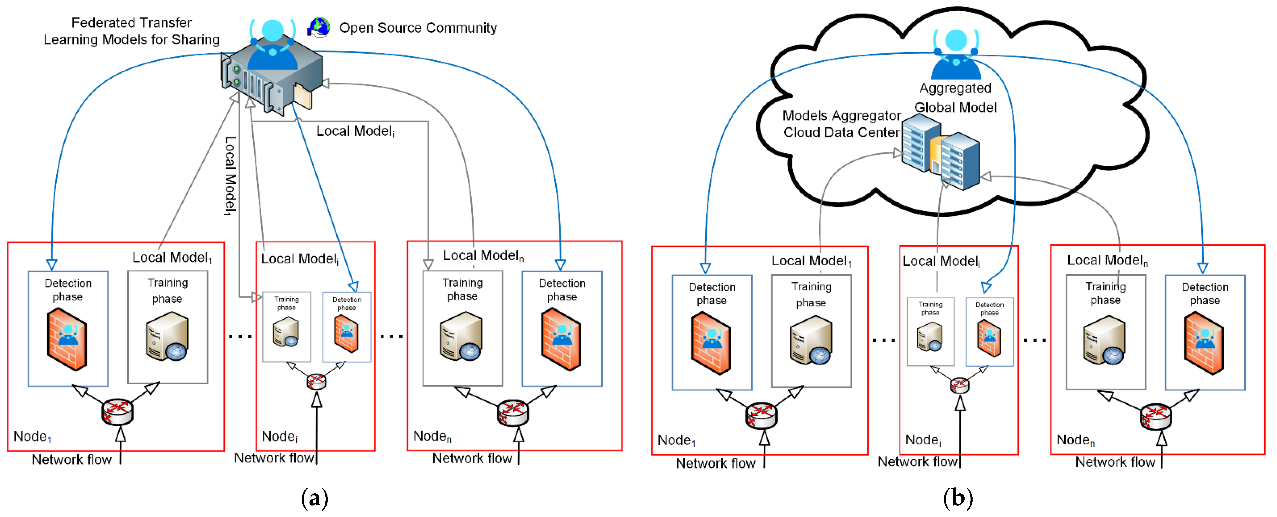
• Stage 1. Participants (in our case nodes) register to an open source community and get the registration number;
• Stage 2. First Local Model training process—the first node₁ trains the model using its own local dataset and then shares the trained local model₁ with the second participant of an open source community;
• Stage 3. Second Local Model training process—the second node₂ downloads the trained local model₁ and uses that model to retrain it with its own local dataset and then shares the trained local model₂ with the next participant of an open source community;
• Stage 4. Next Local Model training process—the next node_i downloads the trained local model₂ and uses that model₂ to retrain it with its own local dataset and then shares the trained local model_i with another participant of an open source community;
• Stage 5. Continuous model retraining process—each participant retrains the model, obtained from its neighbour with its own dataset, and shares the trained model; the process continues until the last registered participant is reached;
• Stage 6. Last Local model training—the last node_n downloads the trained local model_n-1 and uses that model_n-1 to retrain it with its own local dataset and then shares the trained local model_n for sharing with an open source community as a Global Model;

The process of an FL method consists of four stages (see Figure 1b):

• Stage 1. Participant Selection—the server (in our case, Cloud Data Center Model Aggregator) selects a group of participants (in our case, nodes) who meet the prerequisites to participate in the training process;
• Stage 2. Local Models Computation—participants train the local model using their own device’s local dataset. This step is carried out at local nodes;
• Stage 3. Aggregation of Local Models—the server collects enough locally trained deep learning models from participants to update the global deep learning model (the next stage). To prevent the server from analyzing individual deep learning model parameters, this aggregation process must incorporate some privacy-preserving techniques such as safe aggregation, differential privacy, and sophisticated encryption approaches;
• Stage 4. Global Model Update—based on the aggregated model parameters collected in Stage 3, the server updates the current global deep learning model. This revised global model will be sent to participants.

The pseudocode of the FL algorithm for the server (as master), the participating nodes (as workers), and the variants of the aggregate function proposed in [51].

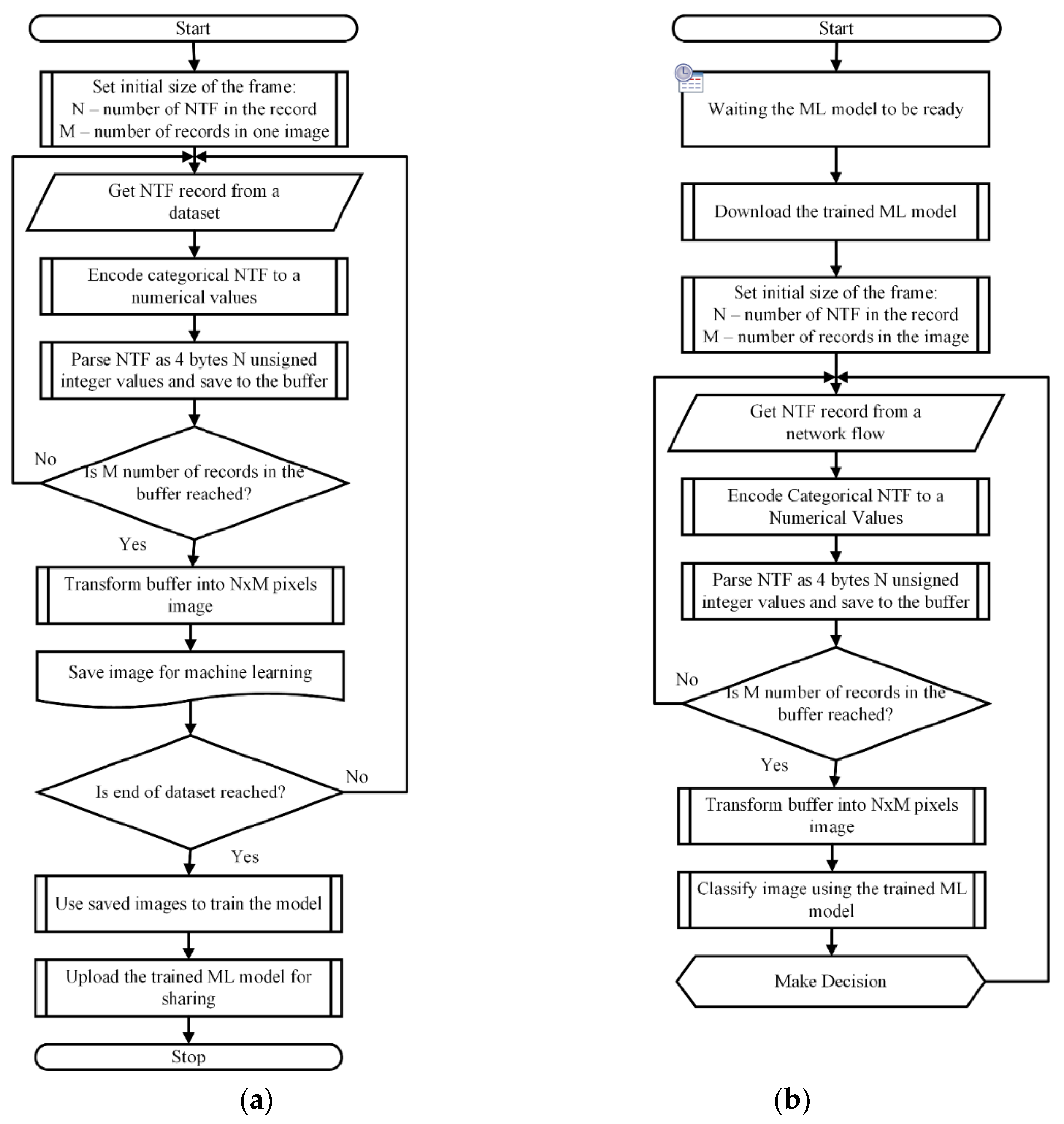
3.1.2. Proposed Method for Framing Network Flow and Representing Frames as Images

There are tons of records of network traffic features (NTF) in a network flow and if we transform records into images, using a one-to-one manner, we will get millions of images for training and recognition. To reduce the number of images, we propose to collect NTF records in a frame and transform the frames into images, so that we will obtain fewer images for training. Obviously, in the frame, only normal traffic records or only attack traffic records or mixed records can be included.

The proposed method for framing NTF records and representing frames as images is shown in Figure 2.

Figure 2. The proposed method for framing records of NTF and representing frames as images: (a) Training phase; (b) Detection phase.

As depicted in Figure 2 for the training phase, the benchmark dataset is used and then the trained model is used for image classification and anomaly detection.

For evaluation of the proposed approach and the comparative study, we performed our experiments in three use cases.

• 1. Traditional transfer learning. Mandatory centralization of training data. Employed DNN with ResNet50 architecture, which allows comparing widely used ML practice with our proposed FTL and FL methods;
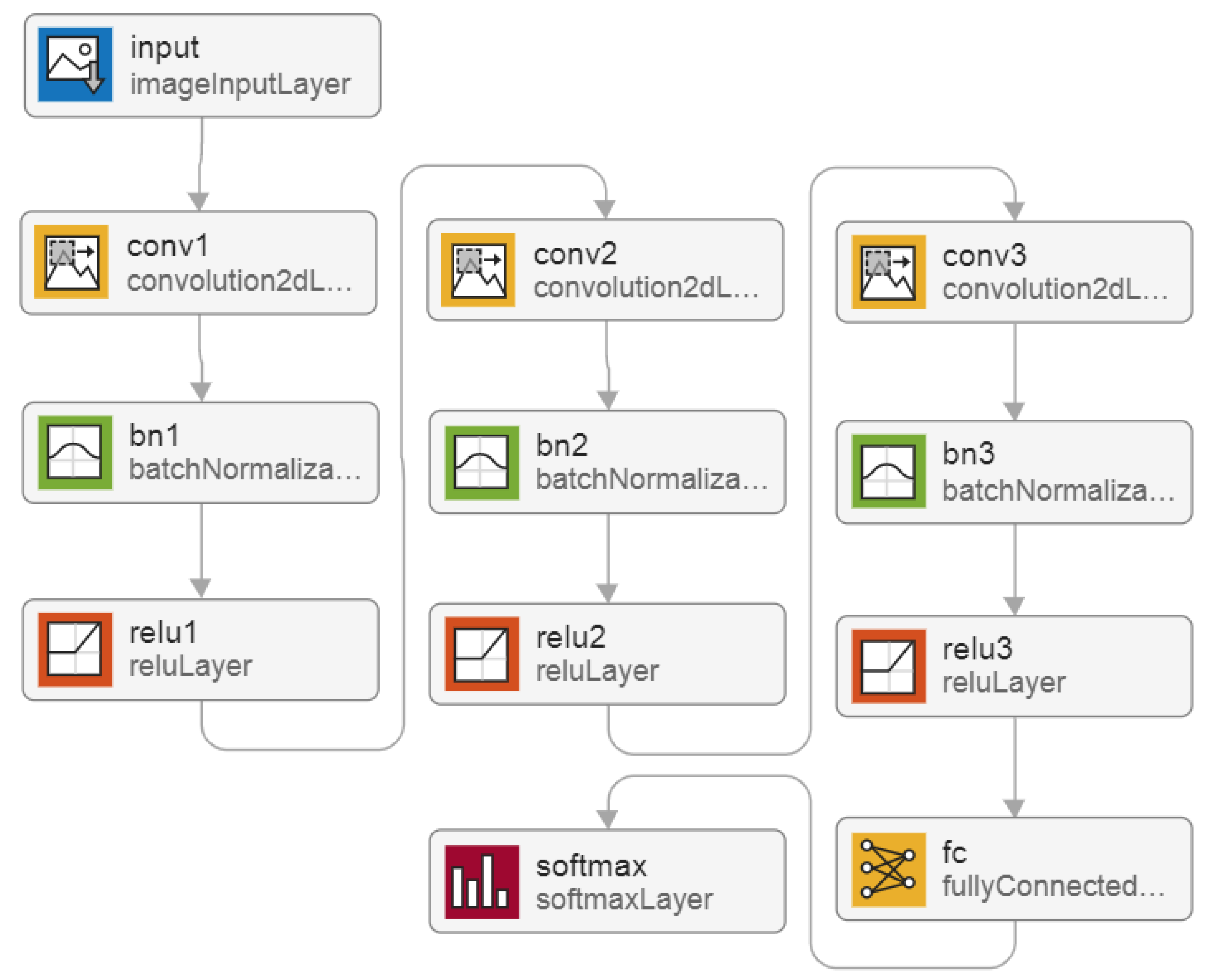
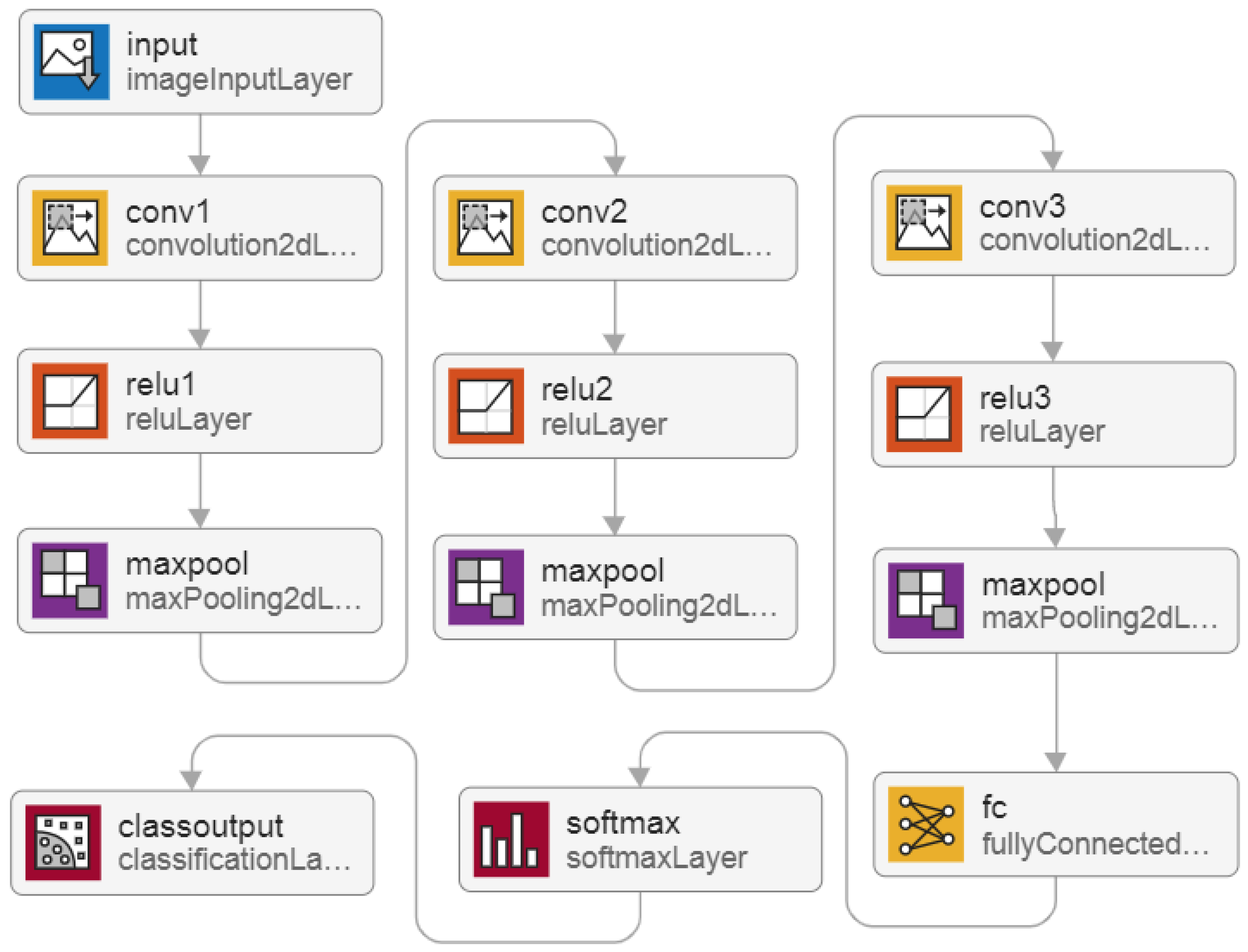
• 2. Federated transfer learning. Training data is disposed at local nodes. Proposed 13-layer DNN architecture. The MATLAB trainNetwork function is used, which trains the models according to the proposed FTL method, as shown in Figure 1a;
• 3. Federated learning. Training data is disposed at local nodes. Proposed 12-layer DNN architecture. The stochastic gradient descent with momentum (SGDM) algorithm is used with a custom training loop, which trains the models according to the proposed FL method, as shown in Figure 1b.

4. Experimental Results

ML models were trained on transformed images using MATLAB. All experiments were carried out on a desktop computer with 64-bit Windows 10 OS with Intel(R) Xeon(R) CPU E5-2630 v2 @ 2.60 GHz (2 processors) with 96 GB RAM and NVIDIA GeForce GTX 1650 SUPER. We use two approaches to train models: transfer learning using the ResnetV2 approach, when 70% of the dataset is used for training purposes and 30% of the dataset is used for testing purposes, and the FL approach, where we use a common dataset to test local models and global models.

4.1. Dataset for Proposed Approach Implementation

As shown in Table 1, various datasets are used to measure the accuracy of network attack recognition. The NSL-KDD benchmark dataset contains four classes of attacks: DoS, Probe, R2L, and U2R. The UNSW-NB15 benchmark dataset contains nine classes of attacks: Analysis, Backdoor, DoS, Exploits, Fuzzers, Generic, Normal, Reconnaissance, Shellcode, and Worms. The two latest proposed benchmark datasets are LITNET-2020 [52] and BOUN-DDoS [53].

For evaluation of the proposed methods, we selected the full BOUN DDoS dataset [53], which has two classes: DDoS attack traffic by flooding TCP SYN and attack-free network traffic. Network-based DDoS intrusion detection techniques or systems can be effectively tested using this. The single victim server that is connected to the campus’s backbone router is the target of the attacks. The attack packets contained spoof source IP addresses that were generated randomly. More than 4000 active hosts were included in the data trace, which was recorded on the backbone. There are tons of NTF records in the BOUN DDoS dataset, which is tremendously more than nine million records (total of 9,335,605). Thus, we propose the NTF records framing method that reduces the number of observations. To simulate federation with its nodes, we create four dataset partitions from the full BOUN DDoS dataset and assume that we have a four-node federation and every node has its own local dataset (in our case partition of the whole BOUN DDoS dataset).

4.2. BOUN-DDoS Dataset Preparation for Experiments

4.2.1. Transformation of NTF Records of the BOUN-DDoS Dataset

Every record of the BOUN-DDoS dataset has 12 NTFs, and four of them are categorical. We transform the NTF records of the BOUN-DDoS dataset into frames and then transform each frame into 32 × 32 pixels images according to the scheme depicted in Figure 3. In the first stage, dataset records are sequentially distributed into frames, where the frame contains 96 NTF records of the BOUN-DDoS dataset (see Figure 3).

Figure 3. Creating images of frames from the BOUN-DDoS dataset NTF records.

The time and frame number are not used because they are not related to the attack properties. The last ten NTFs of the record are 32-bit unsigned integers. Four bytes of every integer represent the values of ARGB image pixels. To create a 32 × 32 pixels image, we construct one row of the ARGB image using 3 NTF records plus two padding integer values (3 × 10 = 30 + 2 = 32) to obtain a 32-byte image width. To create a 32-pixel image height we need to use all 96 NTF records from the image frame: 32 × 3 = 96. An example of transformed NTF frame images is depicted in Figure 4.

Figure 4. Example of transformed NTF records into frame images.

Using the proposed approach, we reduce the number of images 96 times compared to image creation using the one-to-one image creation technique. The creation of one-to-one images produces 9,335,606 images from the full BOUN-DDoS dataset. Using the proposed framing method, the number of transformed images decreases to 97,243. Thus, the computational power and training time can be reduced.

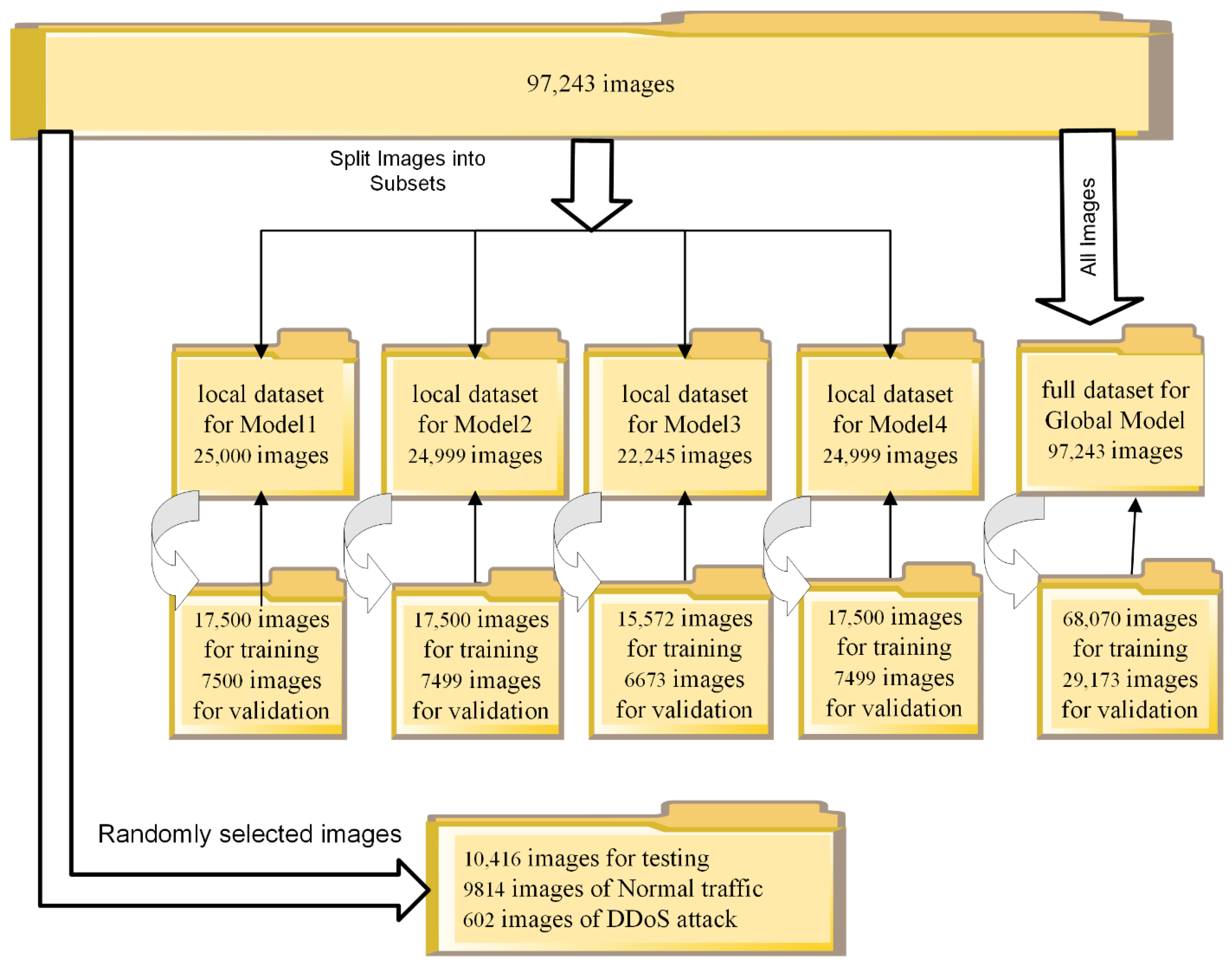
4.2.2. Dataset Partitions for Traditional Transfer Learning Method

We use the definitions of training, validation, and testing datasets as follows:

• Training set. A partition of the dataset used to train, fit, and select the parameters of the model is referred to as the training set. It must reflect the complexity and diversity of the model and often comprises 60 to 70 per cent of the dataset data;
• Validation set. A partition of the dataset used to evaluate the performance of the model while tuning the hyperparameters of the model is referred to as the validation set. The validation set indirectly influences the model, since these data, which typically comprise between 30 and 40% of the dataset data, are used for more frequent evaluation and hyperparameter updates. Although it is typically advised, tuning a model’s hyperparameters is not strictly necessary;
• Testing set. This dataset serves as an objective assessment of how well the model fits the data from the training set. This set is only used after the model has completed the training and does not have a bearing on the model; it is only used to determine performance.

We divide the images into four partition subsets to evaluate the traditional transfer learning process (see Figure 5) using the pre-trained ResNet50 architecture when the subsets were trained locally and the set of all images was trained and validated independently. The ResNet50 architecture contains 50 layers.

Figure 5. Partitioning of images for traditional transfer learning using the ResNet50 architecture.

As depicted in Figure 5, we train all models independently using the traditional transfer learning (TTL) method when 70% of the images from every dataset partition are used for training and 30% of the images from every dataset are used for validation. To test trained models, we create a common testing dataset partition by randomly selecting images from all datasets. It has 10,416 images, where 9814 images represent normal traffic, and 602 images represent DDoS attacks.

4.2.3. Dataset Partitions for Federated Transfer Learning Method

To simulate the FTL method training process (see Figure 6), we use the same local dataset partitions of the full BOUN DDoS dataset that were used for the TTL method with the ResNet50 architecture. The key distinction between the TTL and FTL methods is that FTL models are trained using all images from a local dataset, excluding images from the full dataset, and preserving training data privacy. As depicted in Figure 6, four datasets represent four different nodes, where the nodes train the models sequentially using the trained model shared with the neighbouring node to continue the training process. For all models, the common testing dataset partition as in the previous section (see Figure 5) was used, including 10,416 randomly selected images.

Figure 6. Partitioning of images for FTL method simulation.

The final trained local model is used to construct a Global Model for sharing after FTL is complete. Figure 6 shows that the trained Model4 is being used as a Global Model for sharing.

4.2.4. Dataset Partitions for Federated Learning Method

To simulate the FL method training process, we use the same local dataset partitions of the full BOUN DDoS dataset that were used for the TTL method with the ResNet50 architecture and the FTL method (see Figure 5 and Figure 6). The key distinction between the TTL and FL methods is that FL models are trained using all images from a local dataset, excluding images from the entire dataset, and preserving the privacy of the training data. The key distinction between the FTL and FL methods is that FL models are trained independently and the Global Model for sharing is created by averaging all trained local models as depicted in Figure 7. For all models, the same testing subset of 10,416 randomly selected images as in previous sections (see Figure 5 and Figure 6) was used.

Figure 7. Partitioning of images for FL method simulation.

The Global Model is created by averaging the learnables of all trained local models and evaluated using the dataset with images for validation/testing.

4.3. Experimental Results and Evaluation

We used a confusion matrix to visualize the performance of a supervised learning algorithm for the purpose of evaluating the experimental results. There are four possible classification results, as shown in Figure 8. A true positive (TP) is recorded if the instance is positive and is classified as such; a false negative (FN) is recorded if the classification is negative. Instances that are classified as negative are counted as true negatives (TN); instances that are classified as positive are counted as false positives (FP).

Figure 8. Confusion matrix to visualize the performance of a supervised learning algorithm.

We utilized a common plot created using the MATLAB function confusionchart for the display of the confusion matrix. Each cell’s total number of observations is shown in the confusion matrix. The true class is represented by the rows of the confusion matrix and its columns represent the predicted class. Cells that are diagonal and off-diagonal relate to observations that were correctly and incorrectly categorized, respectively. The percentages of correctly and incorrectly classified observations for each true class are shown in a row-normalized row summary. The percentages of correctly and incorrectly classified observations for each projected class are shown in a column-normalized column summary. Many standard metrics are built on the foundation of this matrix, and we use four metrics to identify the highest performance of the models: accuracy, precision, recall, and F1 score.

Accuracy is defined as follows:

Accuracy = (TN + TP)/(TN + FP + TP + FN),

(1)

Precision is defined as follows:

Precision = TP/(TP + FP),

(2)

Recall is defined as follows:

Recall = TP/(TP + FN),

(3)

F1 score is defined as follows:

F1 score = 2 × (Precision × Recall)/(Precision + Recall),

(4)

In addition, MATLAB provides a loss function and accuracy values during the ML process. An algorithm for ML is optimized using a loss function. The performance of the model in these two sets determines how the loss is calculated, which is based on training and validation data. In training or validation sets, it is the total number of errors produced for each example. The loss value of a model indicates how well or poorly it performs after each optimization cycle. The performance of the algorithm is evaluated using an understandable accuracy metric, which is expressed as a percentage. It measures how closely your model’s forecast matches the actual data.

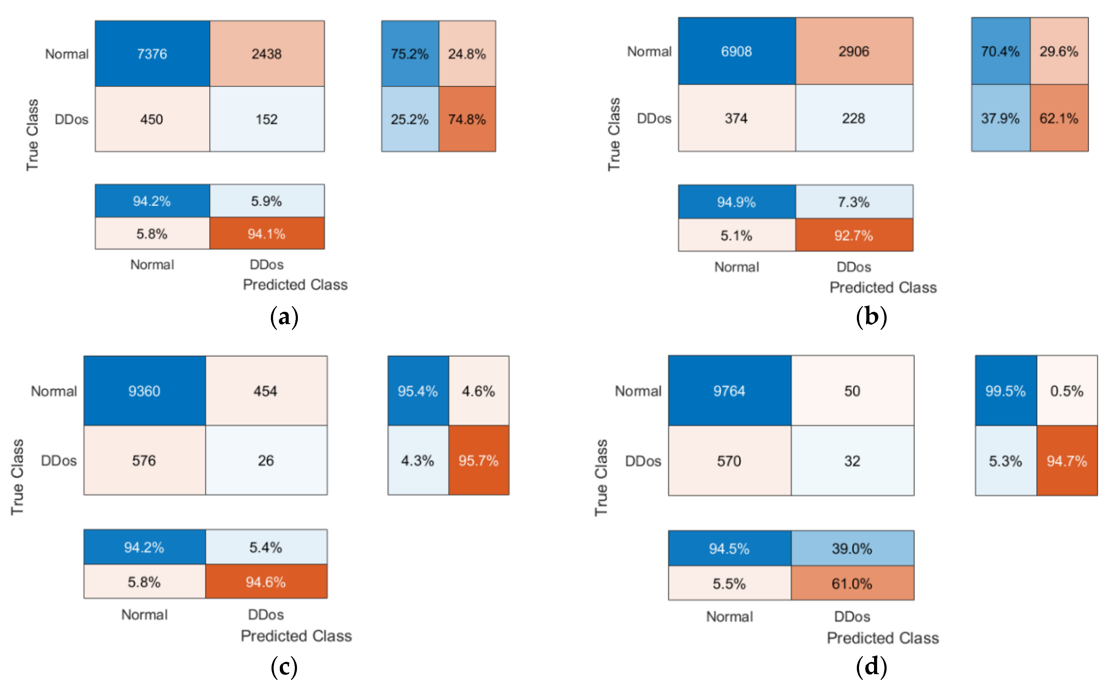
4.3.1. Experimental Results of Traditional Transfer Learning Method

Training options for the TTL with ResNet50 architecture are as follows: initial learn rate 0.001, validation frequency 50, maximum epochs 10, mini-batch size 256, learning dataset of the 70% randomly selected images from the complete training dataset, and validation dataset of the 30% randomly selected images from the complete training dataset. All trained models were tested using a subset of images for testing according to Figure 5.

The confusion matrices visualizing the performance of the TTL with ResNet50 architecture to train local models are presented in Figure 9.

Figure 9. Confusion matrices visualizing the performance of TTL with ResNet50 architecture: (a) for local Model1; (b) for local Model2; (c) for local Model3; (d) for local Model4.

The confusion matrix visualizing the performance of TTL with ResNet50 architecture to train the Global Model (according to Figure 5) is presented in Figure 10.

Figure 10. Confusion matrix visualizing the performance of TTL with ResNet50 architecture to train the Global Model.

The experimental results are summarized in Table 2. Testing accuracy is calculated using Equation (1).

Table 2. Experimental results of the TTL with ResNet50 architecture.

Images Dataset	Most Observations	Fewest Observations	Observations (70%)	Maximum Iterations	Validation Accuracy	Validation Loss	Testing Accuracy	Training Time
Local Model1	Normal (14,657)	DDoS (2843)	17,500	680	86.80%	0.3396	72.27%	9 min 9 s
Local Model2	Normal (14,179)	DDoS (3320)	17,499	680	62.72%	0.4268	68.51%	9 min 23 s
Local Model3	Normal (12,327)	DDoS (3245)	15,572	600	77.64%	0.4419	90.11%	8 min 4 s
Local Model4	Normal (14,668)	DDoS (2832)	17,500	680	83.54%	0.4244	94.05%	9 min 12 s
Global Model	Normal (55,831)	DDoS (12,239)	68,070	2650	80.94%	0.4256	93.95%	43 min 31 s

The results seem to be not so good: the validation accuracy is in the range of 62.72% to 86.80%. The number of observations for the training process was calculated as 70% of every NTF frame images dataset used for training purposes and 30% of each dataset used for validation purposes. The testing accuracy using the common testing dataset (see Figure 5) is in the range of 68.51% to 94.05%. The accuracy of Global Model testing is 93.95%. We assume that the results are not so good for two reasons:

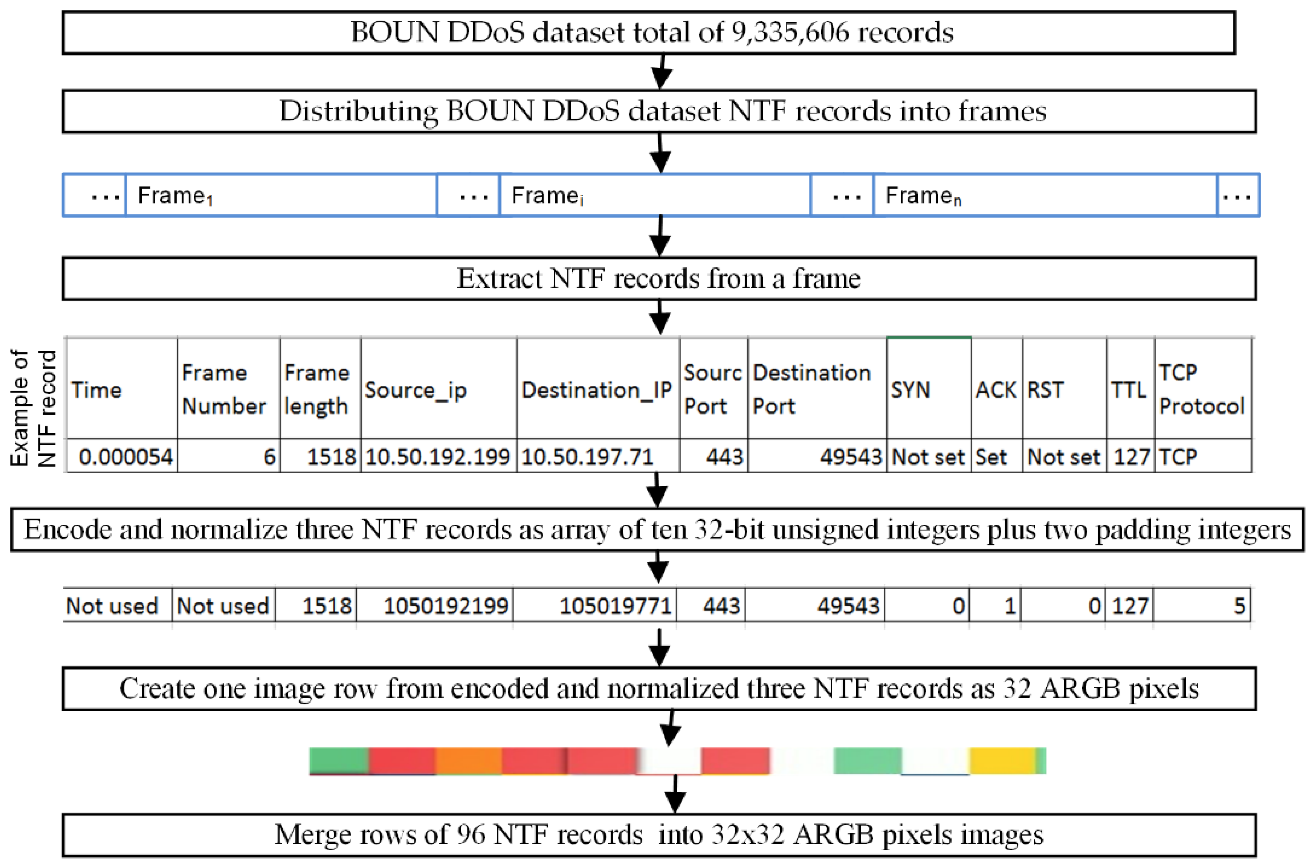
• Distributions of NTF records and combination into frames lead to an overwhelming burst in every frame that distributes 96 NTF records, and thus, each frame can contain normal and DDoS NTF records in any random proportion;
• The ResNet50 architecture contains 50 layers and is very complex and redundant for training a recognition network for the proposed types of images.

To train the Global Model using the TTL method, mandatory data centralization is required and data privacy is not ensured. Moreover, to train the Global Model, the full data set must be used, and the training process requires a lot of computational power and takes a long time. After evaluation and discussion of the mentioned reasons, we decided to employ the DNN architecture and propose the use of FTL and FL methods.

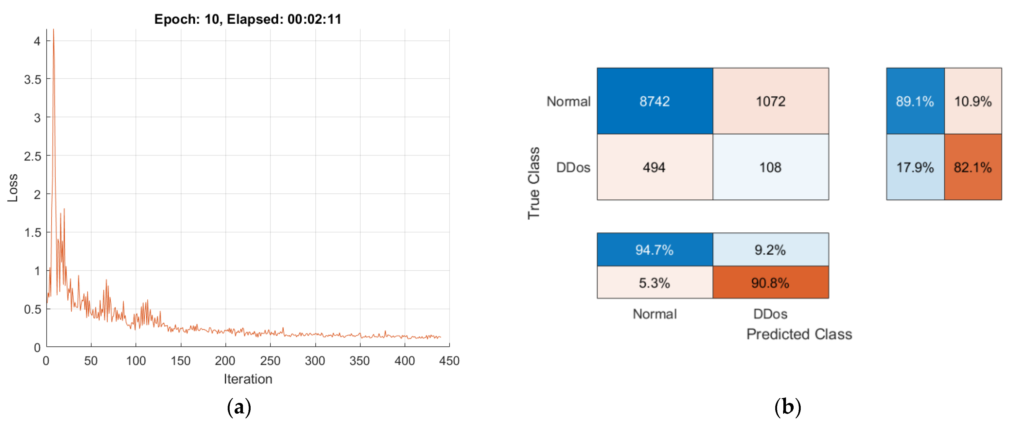
4.3.2. Experimental Results of Federated Transfer Learning Method

To simulate FTL, we propose to use the MATLAB trainNetwork function that trains models according to the suggested FTL method as depicted in Figure 1a and creates the 13-layer DNN architecture depicted in Figure 11.

Figure 11. The 13-layer DNN architecture for the FTL method.

The training options for FTL using the created 13-layer DNN architecture are as follows: learning rate 0.001, validation frequency 50, maximum epochs 10, and the shuffle parameter set to ‘every-epoch’. All frame images in every dataset were used for training as depicted in Figure 6. Exactly: 25,000 images from the dataset for local Model1, 22,499 images from the dataset for local Model2, 22,499 images from the dataset for local Model4, and 22,245 images from the dataset for local Model3 were used.

The FTL training process starts at node₁ using the dataset for local Model1. After the training process in node₁ is completed and the trained local Model1 is created, it is shared with the second node₂. Node₂ continues training using its dataset for local Model2 starting the training process from the trained local Model1. After the training process in node₂ is completed and the trained local Model2 is created, it is shared with the third node₃. Node₃ continues training using its dataset for local Model3 starting the training process from the trained local Model2. After the training process in node₃ is completed and the trained local Model3 is created, it is shared with the fourth node₄. Node₄ continues training using its own dataset for local Model4 starting the training process from the trained local Model3. After the training process in node₄ is completed and the trained local Model4 created, it is treated as the Global Model ready for sharing. The same image dataset was used for validation and testing, as shown in Figure 6.

The confusion matrices visualizing the performance of the FTL method (according to Figure 6) are shown in Figure 12.

Figure 12. Confusion matrices visualizing the performance of the FTL method: (a) for local Model1; (b) for local Model2; (c) for local Model3; (d) for local Model4.

The experimental results of the progress of the proposed FTL method are summarized in Table 3. Testing accuracy was calculated using Equation (1).

Table 3. Experimental results of the proposed FTL method and the 13-layer DNN.

Images Dataset	Most Observations	Fewest Observations	Observations (100%)	Maximum Iterations	Validation Accuracy	Training Error	Testing Accuracy	Training Time
Local Model1	Normal (20,939)	DDoS (4061)	25,000	1950	69.72%	13.18%	69.72%	2 min 50 s
Local Model2	Normal (20,256)	DDoS (4743)	24,999	1950	93.32%	18.63%	93.32%	2 min 55 s
Local Model3	Normal (17,610)	DDoS (4635)	22,245	1730	84.89%	15.37%	84.89%	2 min. 37 s
Local Model4	Normal (20,954)	DDoS (4045)	24,999	1950	92.99%	14.63%	92.99%	2 min 53 s

As we can observe, the validation and testing results are the same because the same dataset was used for validation and testing. According to the proposed FTL method, the local Model4 is treated as a Global Model ready for sharing.

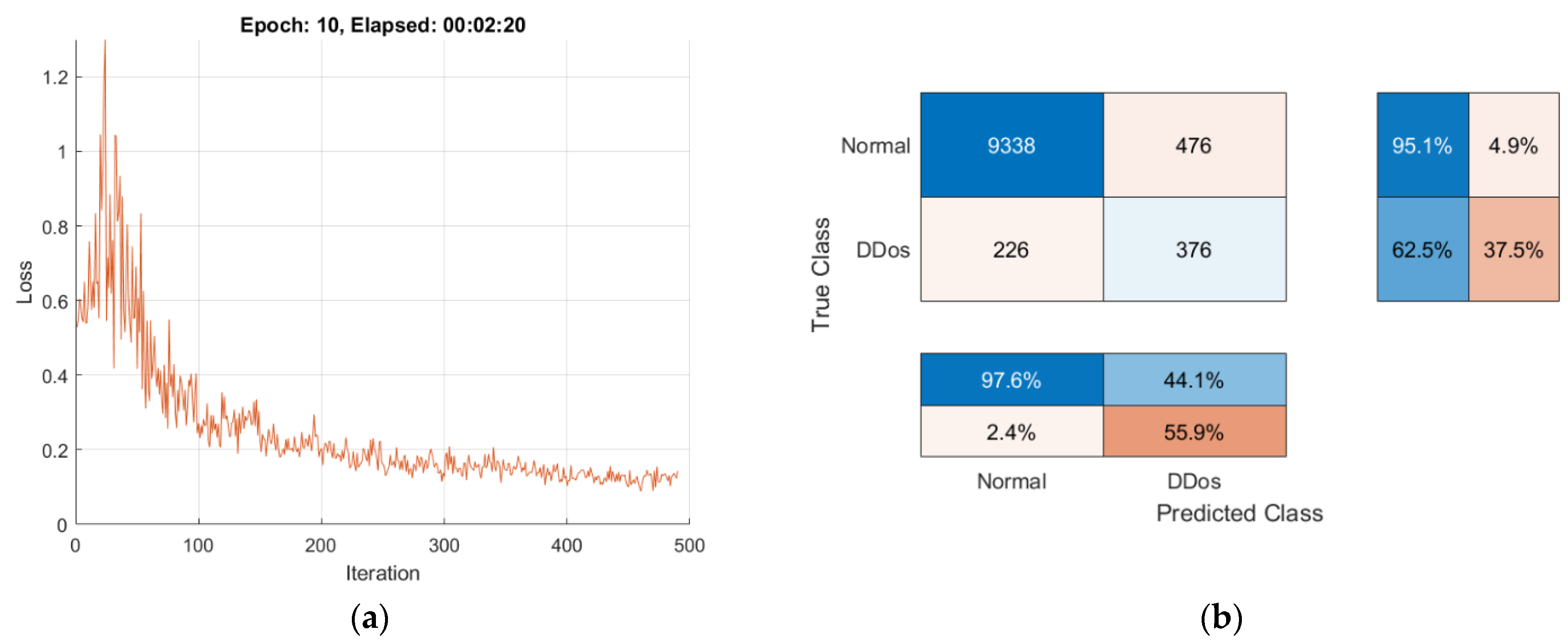
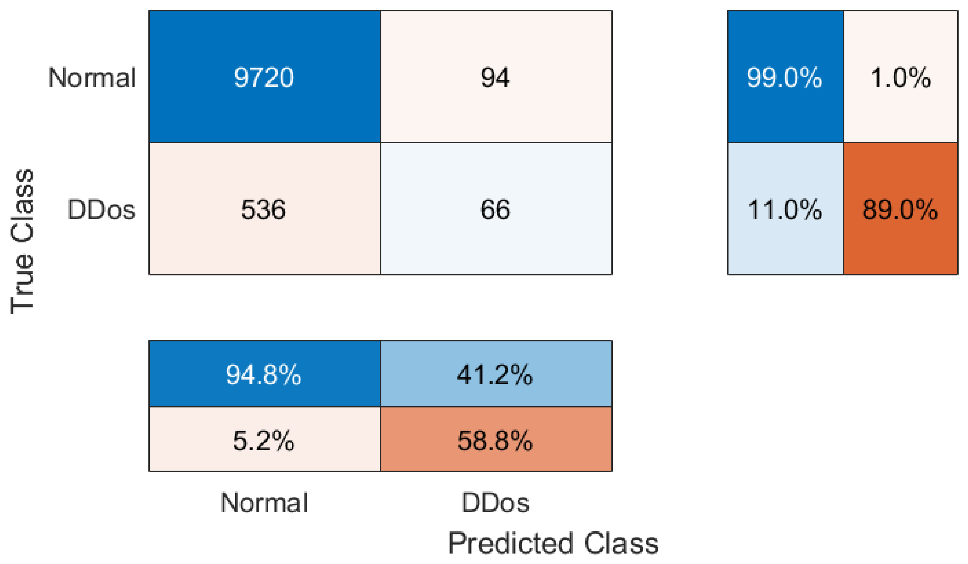
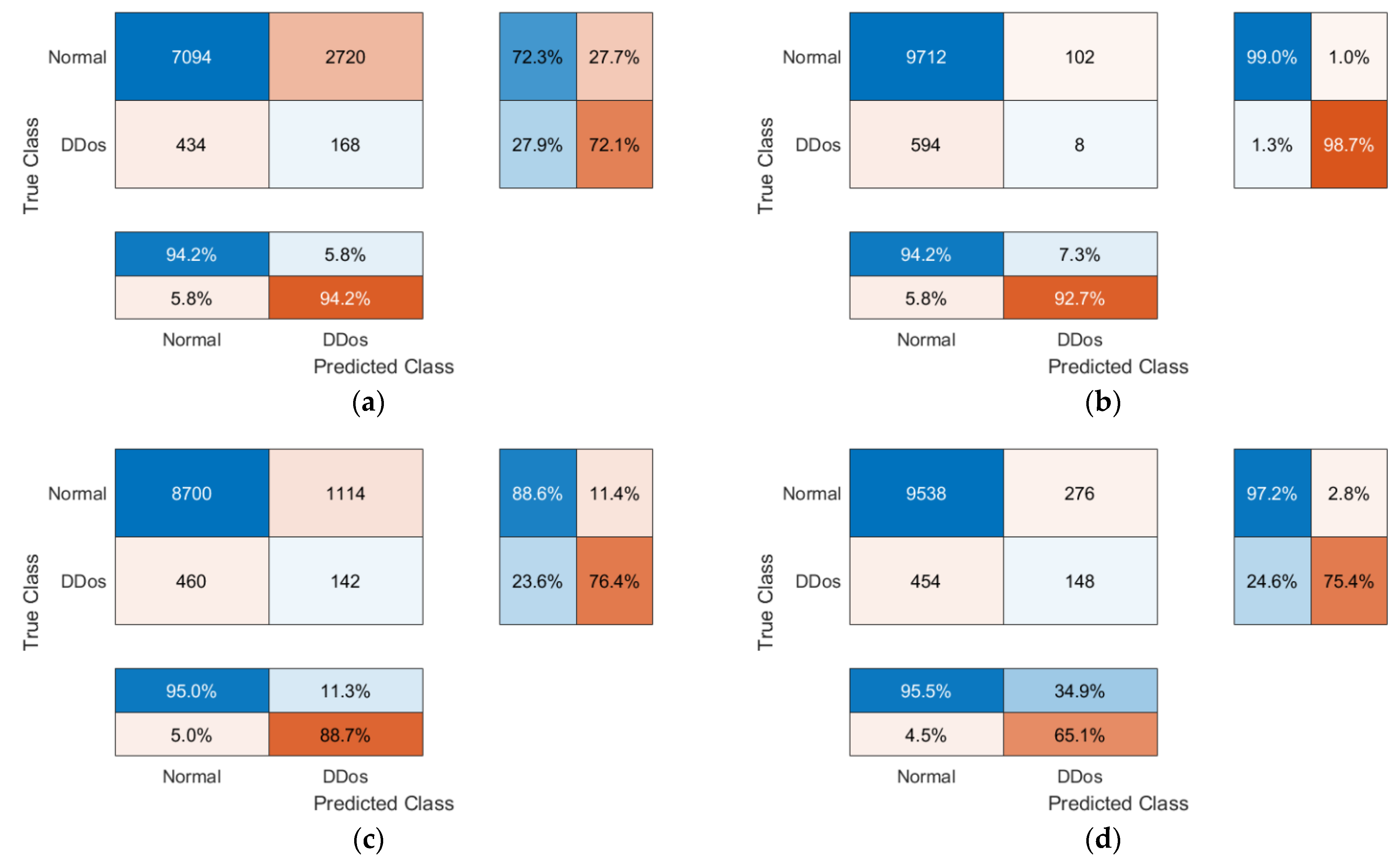
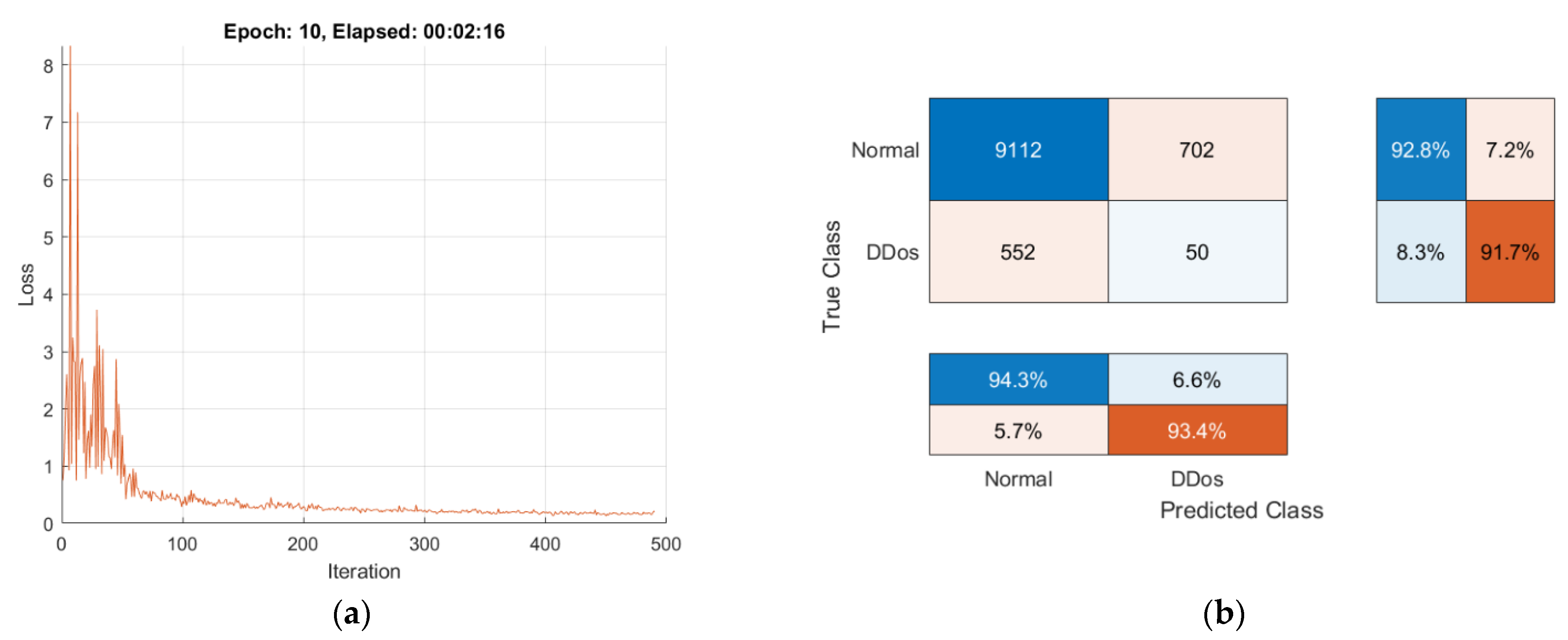
4.3.3. Experimental Results of Federated Learning Method

To simulate the FL method, we propose using the stochastic gradient descent with the momentum (SGDM) algorithm and a custom training loop, which will train the models according to the proposed FL method as depicted in Figure 1b and create the 12-layer DNN architecture depicted in Figure 13.

Figure 13. The 12-layer DNN architecture for the FL method.

We trained the 12-layer DNN with a unique learning rate schedule using the SGDM optimizer to classify images of frames. As a custom learning rate schedule is not available in the trainNetwork function, a custom training loop is created using automated differentiation [54]. The time-based decay learning rate schedule is used in this approach to train a network to classify images. The solver employs the learning rate provided by Equation (5).

N_i = L_r(1 + k × i),

(5)

where, i—is the iteration number, L_r—is the initial learning rate, and k—is the decay.

In order to obtain the gradients of the loss with respect to the learnable parameters in the network and the related loss, we use the function modelGradients [54], which accepts the proposed 12-layer dlnetwork object, a mini-batch of input data, and the corresponding labels. The training parameters for FL using the proposed 12-layer architecture and custom training loop are as follows: initial learn rate 0.001, decay 0.01, momentum 0.9, maximum epochs 10, the shuffle parameter is set to ‘every-epoch’, and mini-batch size 256. The datasets used for learning, validation, and testing are shown in Figure 7. For each epoch, the training loop over mini-batches of data evaluates the model loss, gradients, state, updates the network parameters using the sgdmupdate function, and displays the training progress.

Each local model is trained independently using its own dataset and preserving the privacy of the training data. When the final local model’s training process is finished, an averaged Global Model is created and ready for sharing. Visualizations of the training progress and performance of the FL method are presented in Figure 14, Figure 15, Figure 16 and Figure 17.

Figure 14. Training progress and performance of the FL method: (a) loss evaluation of Local Model1; (b) confusion matrix of Local Model1.

Figure 15. Training progress and performance of the FL method: (a) loss evaluation of Local Model2; (b) confusion matrix of Local Model2.

Figure 16. Training progress and performance of the FL method: (a) loss evaluation of Local Model3; (b) confusion matrix of Local Model3.

Figure 17. Training progress and performance of the FL method: (a) loss evaluation of Local Model4; (b) confusion matrix of Local Model4.

The confusion matrix visualizing the performance of the FL method when testing the aggregated Global Model is shown in Figure 18.

Figure 18. Confusion matrix visualizing the performance testing of the averaged Global Model.

The experimental results of the FL method training progress are summarized in Table 4. Testing accuracy was calculated using Equation (1).

Table 4. Experimental results of training progress using the FL method and the 12-layer DNN.

Images Dataset	Most Observations	Fewest Observations	Observations (100%)	Maximum Iterations	Validation Accuracy	Validation Loss	Testing Accuracy	Training Time
Local Model1	Normal (20,939)	DDoS (4061)	25,000	500	65.57%	0.1873	65.57%	1 min 54 s
Local Model2	Normal (20,256)	DDoS (4743)	24,999	500	87.96%	0.2105	87.96%	2 min 16 s
Local Model3	Normal (17,610)	DDoS (4635)	22,245	500	84.97%	0.1260	84.97%	2 min 11 s
Local Model4	Normal (20,954)	DDoS (4045)	24,999	500	93.26%	0.1436	93.26%	2 min 20 s
Global Average Model	Normal (79,759)	DDoS (17,484)	97,243	-	-	-	88.42%	-

5. Discussion

We evaluate all the obtained results using Equations (1)–(4) and summarize them in Table 5.

Table 5. Evaluation of the experimental results.

Parameter	Local Model1	Local Model2	Local Model3	Local Model4	Global Model
Total No. of images	25,000	24,999	22,245	24,999	97,243
No. of images of Normal traffic	20,939	20,256	17,610	20,954	79,759
No. of images of DDoS attack traffic	4061	4743	4635	4045	17,484
Use case	1. Traditional transfer learning (TTL)
Testing accuracy Equation (1) in %	72.27	68.51	90.11	94.05	93.95
Precision Equation (2) in %	94.25	94.86	94.2	94.48	94.77
Recall Equation (3) in %	75.16	70.39	95.37	99.49	99.04
F1 score Equation (4) in %	83.63	80.81	94.78	96.92	96.86
Training time	9 min 9 s	9 min 23 s	8 min 4 s	9 min 12 s	43 min 31 s
Use case	2. Federated transfer learning (FTL)
Testing accuracy Equation (1) in %	69.72	93.32	84.89	92.99	92.99
Precision Equation (2) in %	94.23	94.24	94.98	95.46	95.46
Recall Equation (3) in %	72.28	98.96	88.65	97.19	97.19
F1 score Equation (4) in %	81.81	96.54	91.7	96.31	96.31
Training time	2 min 50 s	2 min 55 s	2 min 37 s	2 min 53 s	-
Use case	3. Federated learning (FL)
Testing accuracy Equation (1) in %	65.57	87.96	84.97	93.26	88.42
Precision Equation (2) in %	93.47	94.29	94.65	97.64	95
Recall Equation (3) in %	68.23	92.85	89.08	95.15	92.58
F1 score Equation (4) in %	78.88	93.56	91.78	96.38	93.78
Training time	1 min 54 s	2 min 16 s	2 min 11 s	2 min 20 s	-

Evaluating the proposed NTF records framing method to reduce computational power, we can observe the following:

• The BOUN-DDoS dataset (total number of NTF records 9,335,605) is highly imbalanced (this is true for other network intrusion datasets as well) because there is a very small number of NTF records with DDoS attack (125,557) represented as 1.34% compared to NTF records with normal traffic (9,210,048) represented as 98.66%;
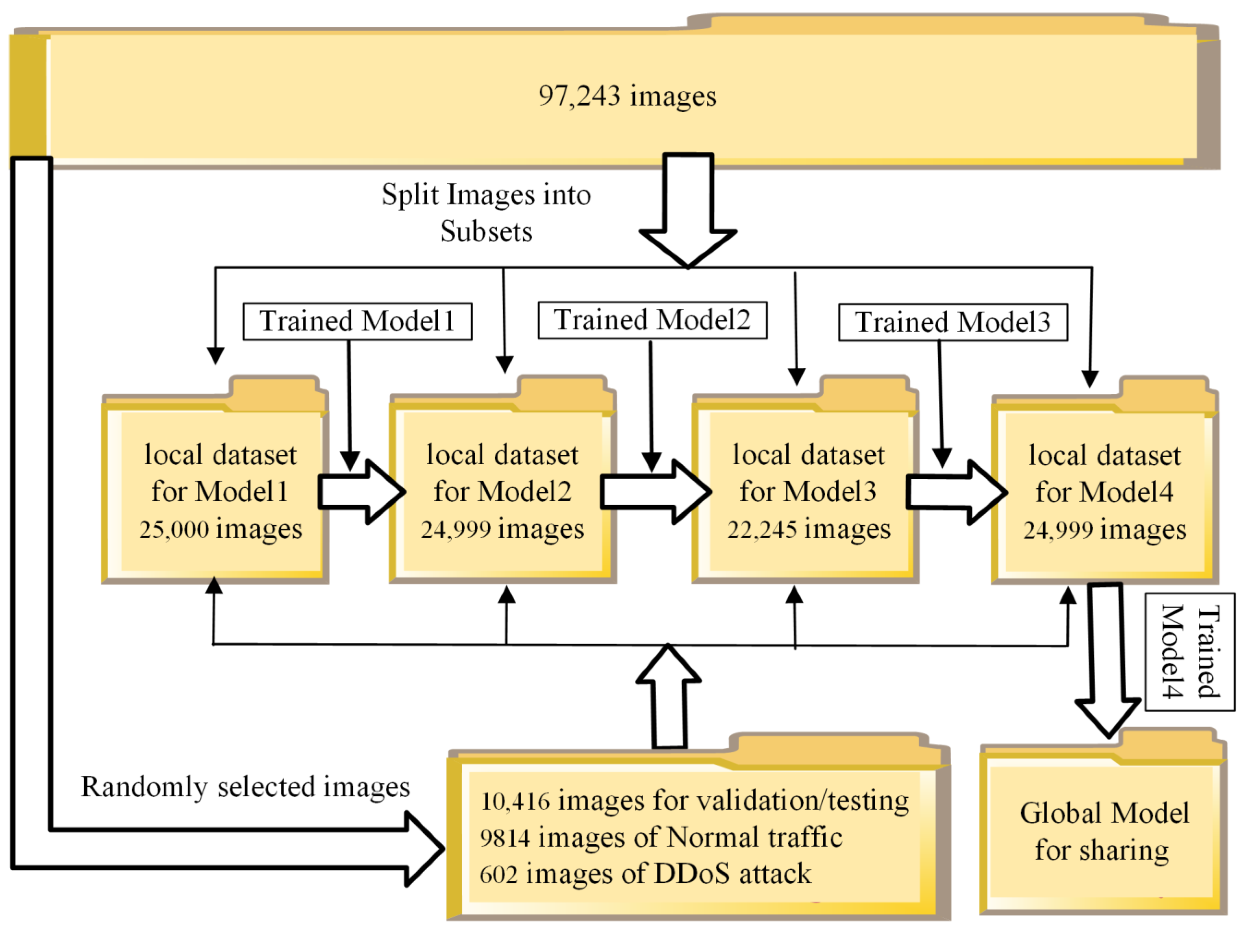
• Framing NTF records into one image reduces the number of images compared to images of NTF records created on a one-to-one basis (in such a case for BOUN DDoS we would have 9,335,605 images). The framing approach reduces the number of images to 97,243–that is, 96 times less;
• On the other hand, framing NTF records into one image makes the ML process complicated because some images represent only NTF records with normal traffic, while others incorporate normal traffic and an unpredictable number of NTF records with DDoS attack. If a DDoS attack takes more than 96 NTF records consistently, such a frame image only represents a DDoS attack.

Evaluating the proposed FTL and FL methods to reduce training time, we can observe the following:

• Compared to FL, the training time for models that utilize TTL with ResNet50 architecture requires more time. It takes roughly 43 min to train a Global Model using a dataset with all 97,243 images when employing TTL. Training local models using the TTL method took more than an hour in total (see Table 2), compared to 12 min when using the FTL method with the 13-layer DNN architecture (see Table 3) and 9 min when using the FL method with the 12-layer DNN architecture (see Table 4). As a result, that is about five times faster than utilizing TTL with ResNet50 architecture.

Evaluating the experimental results of the training progress of the proposed FTL and FL methods, we can observe the following.

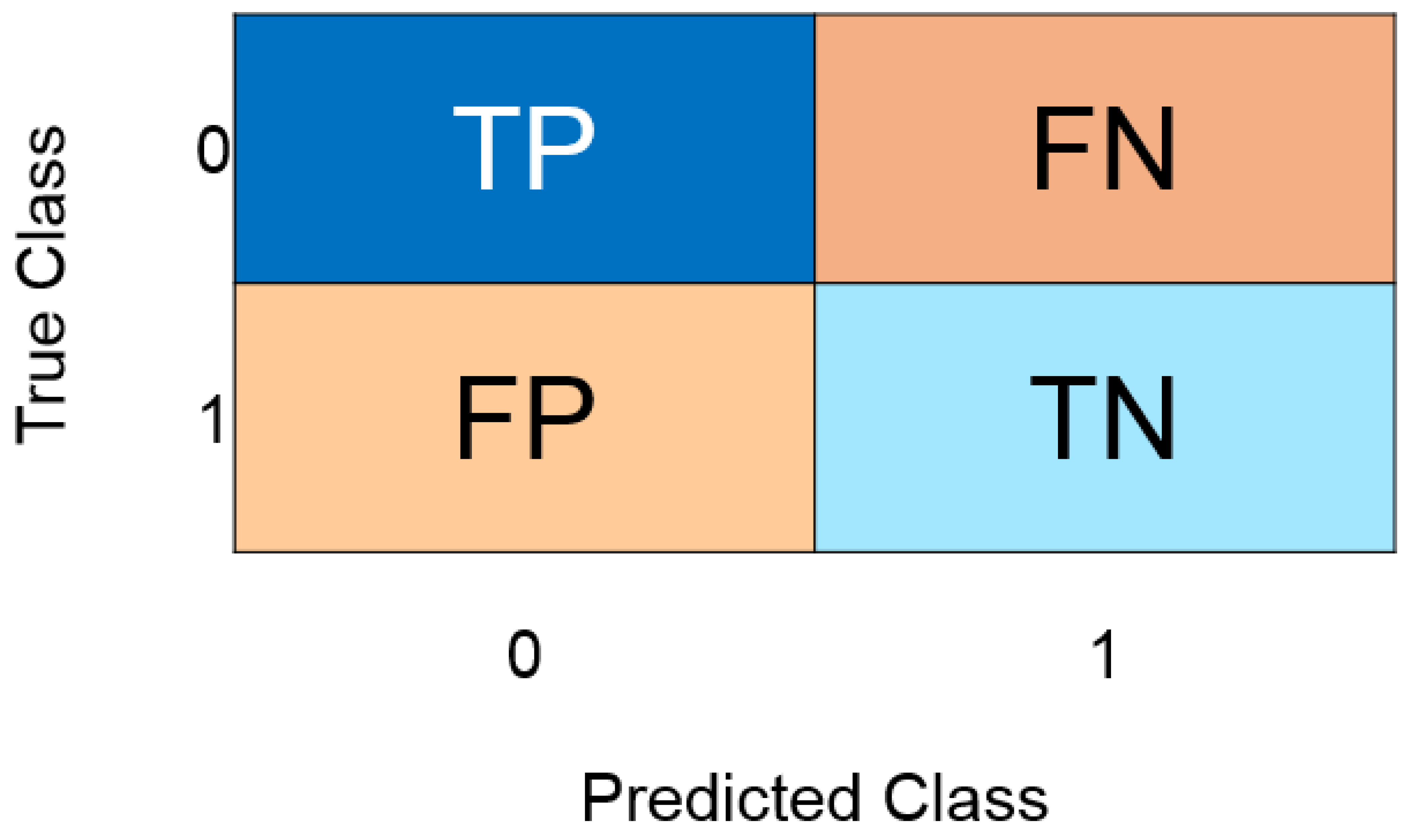
• The number of observations, both positive and negative, that were correctly identified depends on the accuracy. It is a measurement of how closely the model’s forecast matches the actual data. It is simple to obtain a high accuracy score when using accuracy on imbalanced problems by categorizing all observations as belonging to the majority class. Since the testing accuracy of Global Models is strong, ranging from 88.42% to 93.95%, the majority class in our instance is NTF records of normal traffic, and the fundamental challenge to identify normal traffic is being resolved;
• The F1 score, which accounts for both false positives and false negatives, is the weighted average of precision and recall. In most cases, the F1 score is more helpful than accuracy, particularly when the class distribution is imbalanced. The high F1 scores of the Global Models for the suggested FTL method (96.31%) and the FL method (93.78%) are extremely similar to the F1 score for the TTL with ResNet50 architecture (96.86%).

Evaluating the performance of the proposed FTL and FL methods testing vs. privacy, we can observe the following:

• Using the proposed FTL and FL methods for training does not require data centralization and preserves participant data privacy while obtaining nearly the same Global Models testing results in accuracy and F1 score as using the TTL method.
• We can notice that local model testing occasionally yields better testing results when we compare the results of testing local models with those of testing Global Models. When all participants use the Global Model instead of their local models, participant privacy is guaranteed, even though the use of the global model may be superior for some participants while being poorer for others.

Future work will involve suggesting a strategy for developing a dynamic frame creation approach that uses moving windows through NTF records.

6. Conclusions

Building NIDS effectively requires the application of deep learning techniques, which is not an easy undertaking given how crucial NIDS are to cybersecurity. In this article, we investigate three distinct machine learning (ML) methods: Traditional transfer learning (TTL), Federated transfer learning (FTL), and Federated learning (FL). In this work, we propose how to create datasets for FL simulation utilizing big, already-existing BOUN-DDoS datasets for federated learning experiments, and framing NTF records into one image method to reduce the number of images for ML. The complexity of the network, the number of layers, and the number of neurons in each layer often influence training and testing (inference) time.

Researchers must consider the trade-offs between accuracy and model complexity. As a result, we recommended employing the proposed NTF records preprocessing method, which simplifies the network architecture and minimizes computational complexity. Our experiments show that acceptable results with fast convergence can be obtained by reducing model training time: the number of training epochs (10 epochs in our experiments) and the time required to achieve a model’s average accuracy (epochs to convergence).

When FL simulation datasets are used to solve the NIDS problem, the FL model based on deep learning exhibits a classification performance that is comparable to that of the centralized TTL. The suggested FTL and FL methods differ from the TTL strategy in that they avoid the need to transfer data to a centralized server, preserving user privacy—which is crucial for this particular situation. The experimental investigation shows how both FTL and FL contribute to preserving privacy without significantly lowering accuracy and F1-score. Framing NTF records into one image method realized in C# programming language has a possibility of hardware implementation employing NET Framework Common Language Runtime.

References

- Bhuyan, M.H.; Bhattacharyya, D.K.; Kalita, J.K. Network Anomaly Detection: Methods, Systems and Tools. IEEE Commun. Surv. Tutor. 2014, 16, 303–336. [Google Scholar] [CrossRef]
- Zhang, H.; Li, J.; Liu, X.; Dong, C. Multi-dimensional feature fusion and stacking ensemble mechanism for network intrusion detection. Future Gen. Comput. Syst. 2021, 122, 130–143. [Google Scholar] [CrossRef]
- Aljanabi, M.; Ismail, M.A.; Ali, A.H. Intrusion Detection Systems, Issues, Challenges, and Needs. Int. J. Comput. Intell. Syst. 2021, 14, 560–571. [Google Scholar] [CrossRef]
- Pontes, C.; Souza, M.; Gondim, J.; Bishop, M.; Marotta, M. A new method for flow-based network intrusion detection using the inverse Potts model. IEEE Trans. Netw. Serv. Manag. 2021, 18, 1125–1136. [Google Scholar] [CrossRef]
- Umer, M.; Sher, M.; Bi, Y. Flow-based intrusion detection: Techniques and challenges. Comput. Secur. 2017, 70, 238–254. [Google Scholar] [CrossRef]
- Song, S.; Ling, L.; Manikopoulo, C.N. Flow-based Statistical Aggregation Schemes for Network Anomaly Detection. In Proceedings of the 2006 IEEE International Conference on Networking, Sensing and Control, Ft. Lauderdale, FL, USA, 23–25 April 2006; pp. 786–791. [Google Scholar] [CrossRef]
- Cisco Annual Internet Report (2018–2023) White Paper. Available online: https://www.cisco.com/c/en/us/solutions/collateral/executive-perspectives/annual-internet-report/white-paper-c11-741490.html (accessed on 11 August 2022).
- Das, A.; Balakrishnan, S.G. A Comparative Analysis of Deep Learning Approaches in Intrusion Detection System. In Proceedings of the 2021 International Conference on Recent Trends on Electronics, Information, Communication & Technology (RTEICT), Bangalore, India, 27–28 August 2021; pp. 555–562. [Google Scholar] [CrossRef]
- Ahmad, Z.; Shahid Khan, A.; Wai Shiang, C.; Abdullah, J.; Ahmad, F. Network intrusion detection system: A systematic study of machine learning and deep learning approaches. Trans. Emerg. Tel. Tech 2021, 32, e4150. [Google Scholar] [CrossRef]
- Albulayhi, K.; Smadi, A.A.; Sheldon, F.T.; Abercrombie, R.K. IoT intrusion detection taxonomy, reference architecture, and analyses. Sensors 2021, 21, 6432. [Google Scholar] [CrossRef]
- Lee, S.; Mohammed sidqi, H.; Mohammadi, M.; Rashidi, S.; Rahmani, A.M.; Masdari, M.; Hosseinzadeh, M. Towards secure intrusion detection systems using deep learning techniques: Comprehensive analysis and review. J. Netw. Comput. Appl. 2021, 187, 103111. [Google Scholar] [CrossRef]
- Rabbani, M.; Wang, Y.; Khoshkangini, R.; Jelodar, H.; Zhao, R.; Ahmadi, S.B.B.; Ayobi, S. A review on machine learning approaches for network malicious behavior detection in emerging technologies. Entropy 2021, 23, 529. [Google Scholar] [CrossRef]
- Jordan, M.I.; Mitchell, T.M. Machine learning: Trends, perspectives, and prospects. Science 2015, 349, 255–260. [Google Scholar] [CrossRef]
- Lecun, Y.; Bengio, Y.; Hinton, G. Deep learning. Nature 2015, 521, 436–444. [Google Scholar] [CrossRef] [PubMed]
- Arulkumaran, K.; Deisenroth, M.P.; Brundage, M.; Bharath, A.A. Deep reinforcement learning: A brief survey. IEEE Signal Process. Mag. 2017, 34, 26–38. [Google Scholar] [CrossRef]
- Pan, S.J.; Yang, Q. A survey on transfer learning. IEEE Trans. Knowl. Data Eng. 2010, 22, 1345–1359. [Google Scholar] [CrossRef]
- Kairouz, P.; McMahan, H.B.; Avent, B.; Bellet, A.; Bennis, M.; Bhagoji, A.N.; Zhao, S. Advances and Open Problems in Federated Learning; Now Foundations and Trends: Boston, MA, USA, 2021. [Google Scholar] [CrossRef]
- Lo, S.K.; Lu, Q.; Wang, C.; Paik, H.; Zhu, L. A systematic literature review on federated machine learning: From a software engineering perspective. ACM Comput. Surv. 2022, 54, 1–39. [Google Scholar] [CrossRef]
- Yin, X.; Zhu, Y.; Hu, J. A comprehensive survey of privacy-preserving federated learning: A taxonomy, review, and future directions. ACM Comput. Surv. 2022, 54, 1–36. [Google Scholar] [CrossRef]
- Zerka, F.; Barakat, S.; Walsh, S.; Bogowicz, M.; Leijenaar, R.T.H.; Jochems, A.; Lambin, P. Systematic review of privacy-preserving distributed machine learning from federated databases in health care. JCO Clin. Cancer Inform. 2020, 3, 184–200. [Google Scholar] [CrossRef]
- Jiang, J.C.; Kantarci, B.; Oktug, S.; Soyata, T. Federated learning in smart city sensing: Challenges and opportunities. Sensors 2020, 20, 6230. [Google Scholar] [CrossRef]
- Nguyen, T.D.; Marchal, S.; Miettinen, M.; Fereidooni, H.; Asokan, N.; Sadeghi, A. DÏoT: A federated self-learning anomaly detection system for IoT. In Proceedings of the International Conference on Distributed Computing Systems, Dallas, TX, USA, 7–10 July 2019; pp. 756–767. [Google Scholar] [CrossRef]
- Qu, Y.; Pokhrel, S.R.; Garg, S.; Gao, L.; Xiang, Y. A blockchained federated learning framework for cognitive computing in industry 4.0 networks. IEEE Trans. Ind. Inform. 2021, 17, 2964–2973. [Google Scholar] [CrossRef]
- Aledhari, M.; Razzak, R.; Parizi, R.M.; Saeed, F. Federated learning: A survey on enabling technologies, protocols, and applications. IEEE Access 2020, 8, 140699–140725. [Google Scholar] [CrossRef]
- Sheth, A.P.; Larson, J.A. Federated database systems for managing distributed, heterogeneous, and autonomous databases. ACM Comput. Surv. (CSUR) 1990, 22, 183–236. [Google Scholar] [CrossRef]
- Kurze, T.; Klems, M.; Bermbach, D.; Lenk, A.; Tai, S.; Kunze, M. Cloud federation. In Proceedings of the CLOUD COMPUTING 2011: The Second International Conference on Cloud Computing, GRIDs, and Virtualization, Rome, Italy, 25–30 September 2011; pp. 32–38. [Google Scholar]
- Xu, S.; Qian, Y.; Hu, R.Q. Data-driven edge intelligence for robust network anomaly detection. IEEE Trans. Netw. Sci. Eng. 2019, 7, 1481–1492. [Google Scholar] [CrossRef]
- Preuveneers, D.; Rimmer, V.; Tsingenopoulos, I.; Spooren, J.; Joosen, W.; Ilie-Zudor, E. Chained anomaly detection models for federated learning: An intrusion detection case study. NATO Adv. Sci. Inst. Ser. E Appl. Sci. 2018, 8, 2663. [Google Scholar] [CrossRef]
- Aliyu, I.; Feliciano, M.C.; Van Engelenburg, S.; Kim, D.O.; Lim, C.G. A blockchain-based federated forest for SDN-enabled in-vehicle network intrusion detection system. IEEE Access 2021, 9, 102593–102608. [Google Scholar] [CrossRef]
- Cetin, B.; Lazar, A.; Kim, J.; Sim, A.; Wu, K. Federated wireless network intrusion detection. In Proceedings of the 2019 IEEE International Conference on Big Data, Los Angeles, CA, USA, 9–12 December 2019; pp. 6004–6006. [Google Scholar] [CrossRef]
- Huong, T.T.; Bac, T.P.; Long, D.M.; Thang, B.D.; Binh, N.T.; Luong, T.D.; Phuc, T.K. LocKedge: Low-complexity cyberattack detection in IoT edge computing. IEEE Access 2021, 9, 29696–29710. [Google Scholar] [CrossRef]
- Li, K.; Zhou, H.; Tu, Z.; Wang, W.; Zhang, H. Distributed network intrusion detection system in satellite-terrestrial integrated networks using federated learning. IEEE Access 2020, 8, 214852–214865. [Google Scholar] [CrossRef]
- Nguyen, D.C.; Ding, M.; Pathirana, P.N.; Seneviratne, A.; Li, J.; Vincent Poor, H. Federated learning for internet of things: A comprehensive survey. IEEE Commun. Surv. Tutor. 2021, 23, 1622–1658. [Google Scholar] [CrossRef]
- Qin, Q.; Poularakis, K.; Leung, K.K.; Tassiulas, L. Line-speed and scalable intrusion detection at the network edge via federated learning. In Proceedings of the IFIP Networking 2020 Conference and Workshops, Paris, France, 22–26 June 2020; pp. 352–360. [Google Scholar]
- Shi, J.; Ge, B.; Liu, Y.; Yan, Y.; Li, S. Data privacy security guaranteed network intrusion detection system based on federated learning. In Proceedings of the IEEE Conference on Computer Communications Workshops, INFOCOM WKSHPS 2021, Vancouver, BC, Canada, 10–13 May 2021. [Google Scholar] [CrossRef]
- Tian, Q.; Guang, C.; Chen, W.; Si, W. A lightweight residual networks framework for DDoS attack classification based on federated learning. In Proceedings of the IEEE Conference on Computer Communications Workshops, INFOCOM WKSHPS 2021, Vancouver, BC, Canada, 10–13 May 2021. [Google Scholar] [CrossRef]
- Xie, B.; Dong, X.; Wang, C. An improved K-means clustering intrusion detection algorithm for wireless networks based on federated learning. Wirel. Commun. Mob. Comput. 2021, 2021, 9322368. [Google Scholar] [CrossRef]
- Rahman, S.A.; Tout, H.; Talhi, C.; Mourad, A. Internet of things intrusion detection: Centralized, on-device, or federated learning? IEEE Netw. 2020, 34, 310–317. [Google Scholar] [CrossRef]
- Saadat, H.; Aboumadi, A.; Mohamed, A.; Erbad, A.; Guizani, M. Hierarchical federated learning for collaborative IDS in IoT applications. In Proceedings of the 10th Mediterranean Conference on Embedded Computing, MECO 2021, Budva, Montenegro, 7–10 June 2021. [Google Scholar] [CrossRef]
- Hemalatha, J.; Roseline, S.A.; Geetha, S.; Kadry, S.; Damaševičius, R. An efficient densenet-based deep learning model for malware detection. Entropy 2021, 23, 344. [Google Scholar] [CrossRef]
- Awan, M.J.; Masood, O.A.; Mohammed, M.A.; Yasin, A.; Zain, A.M.; Damaševičius, R.; Abdulkareem, K.H. Image-based malware classification using vgg19 network and spatial convolutional attention. Electronics 2021, 10, 2444. [Google Scholar] [CrossRef]
- Azeez, N.A.; Odufuwa, O.E.; Misra, S.; Oluranti, J.; Damaševičius, R. Windows PE malware detection using ensemble learning. Informatics 2021, 8, 10. [Google Scholar] [CrossRef]
- Damaševičius, R.; Venčkauskas, A.; Toldinas, J.; Grigaliūnas, Š. Ensemble-based classification using neural networks and machine learning models for windows pe malware detection. Electronics 2021, 10, 485. [Google Scholar] [CrossRef]
- Toldinas, J.; Venčkauskas, A.; Damaševičius, R.; Grigaliūnas, Š.; Morkevičius, N.; Baranauskas, E. A novel approach for network intrusion detection using multistage deep learning image recognition. Electronics 2021, 10, 1854. [Google Scholar] [CrossRef]
- Alharbi, A.; Alosaimi, W.; Alyami, H.; Rauf, H.T.; Damaševičius, R. Botnet attack detection using local global best bat algorithm for industrial internet of things. Electronics 2021, 10, 1341. [Google Scholar] [CrossRef]
- Islam, A.; Al Amin, A.; Shin, S.Y. FBI: A Federated Learning-Based Blockchain-Embedded Data Accumulation Scheme Using Drones for Internet of Things. IEEE Wirel. Commun. Lett. 2022, 11, 972–976. [Google Scholar] [CrossRef]
- Chen, J.; Li, J.; Huang, R.; Yue, K.; Chen, Z.; Li, W. Federated Transfer Learning for Bearing Fault Diagnosis With Discrepancy-Based Weighted Federated Averaging. IEEE Trans. Instrum. Meas. 2022, 71, 3514911. [Google Scholar] [CrossRef]
- Li, Q.; Wen, Z.; Wu, Z.; Hu, S.; Wang, N.; Li, Y.; Liu, X.; He, B. A Survey on Federated Learning Systems: Vision, Hype and Reality for Data Privacy and Protection. IEEE Trans. Knowl. Data Eng. 2021. [Google Scholar] [CrossRef]
- Voigt, P.; von dem Bussche, A. The EU General Data Protection Regulation (GDPR). In A Practical Guide, 1st ed.; Springer International Publishing: Cham, Switzerland, 2017. [Google Scholar]
- Pardau, S.L. The California Consumer Privacy Act: Towards A European-Style Privacy Regime in the United States? J. Technol. Law Policy 2018, 23, 68. Available online: https://scholarship.law.ufl.edu/jtlp/vol23/iss1/2 (accessed on 26 September 2022).
- Hegedűs, I.; Danner, G.; Jelasity, M. Decentralized learning works: An empirical comparison of gossip learning and federated learning. J. Parallel Distrib. Comput. 2021, 148, 109–124. [Google Scholar] [CrossRef]
- Damasevicius, R.; Venckauskas, A.; Grigaliunas, S.; Toldinas, J.; Morkevicius, N.; Aleliunas, T.; Smuikys, P. LITNET-2020: An Annotated Real-World Network Flow Dataset for Network Intrusion Detection. Electronics 2020, 9, 800. [Google Scholar] [CrossRef]
- Erhan, D.; Anarım, E. Boğaziçi University distributed denial of service dataset. Data Brief. 2020, 32, 106187. [Google Scholar] [CrossRef] [PubMed]
- Train Network Using Custom Training Loop. Available online: https://se.mathworks.com/help/deeplearning/ug/train-network-using-custom-training-loop.html (accessed on 26 May 2022).