1. Introduction
1.1. Background
Electricity markets are competitive markets, usually in the form of financial swaps, that allow buyers and sellers to make bid purchases, offers, and short-term transactions. Faced with the new situation of all kinds of electricity sellers participating in electricity market transactions, it is a key issue for electricity companies to build a bidding strategy and maximize revenue. Researching scientific electricity declaration and price decision-making methods is of great significance and value for e-commerce retailers to optimize their own behavior strategies and optimize the allocation of market resources [
1,
2].
When faced with the problem of new energy consumption, the electricity market adopts the form of guaranteed consumption in the early stage of market construction and development, that is, the power company purchases it to the trading center. The price of the unified purchase is usually set by the government and appropriate compensation is given. With the increasing volume of new energy in the district, the unified purchase transaction mode of guaranteed consumption has caused huge pressure on the power grid. Therefore, it is of great significance to slowly explore new New-energy consumption policies, incorporate new energy consumption into the scope of market competition, and ensure the competitiveness of the new energy market while promoting the combination of new energy consumption and the power market [
3,
4].
Nash equilibrium is the basic theory in game theory. It was originally proposed by American mathematician Nash. The theory points out that all players cannot obtain greater benefits by unilaterally changing their strategies, so this strategy combination is the Nash equilibrium of the game. Under the mechanism of free quotation, every rational generator hopes to maximize its own income through strategic quotation, and finally reach the Nash equilibrium point of the game [
5]. In game theory, the electricity market composed of competing and influencing power generators forms a non-cooperative game, and the corresponding market Nash equilibrium is a very attractive market result. This is because all power generators have no motive to unilaterally change their bidding strategies at the Nash equilibrium, which means that as long as power generators choose the strategy at the market equilibrium, the power market operation will reach a stable state. result of the operation. Therefore, in the market environment, it is very important for power generators to adopt a reasonable bidding strategy. Power generators can ultimately change their own income by changing their bidding strategies, and must also consider the impact of other manufacturers’ changing bidding strategies on their own interests [
6].
The most common way to formulate supplier bidding strategies is to build game theory models [
7]. The most widely used game theory method is based on the Karush-Kuhn-Tucker (KKT) condition. It models the problem as an Equilibrium Problem with Equilibrium Constraints (EPEC). To build a game-theoretic model, a supplier should have a global view of the system and its opponents, such as the location marginal price (LMP) of other nodes, bidding behavior and the cost function of its opponents. External information available to generation suppliers is often limited, making this analytical approach impractical.
The decision-making process of a single strategic power generation company is usually modeled by a two-layer optimization model [
8,
9], which captures the strategic players (modeled at the upper layer (UL)) and the market competition clearing (in the lower layer (LL) modeling). Two-layer optimization problems are usually solved after transforming them into single-layer mathematical programming with equilibrium constraints (MPEC), which are replaced by their equivalent KKT optimality conditions. This idea constitutes the core framework for studying the optimal strategies of generators and the multi-generator Nash equilibrium strategies derived therefrom. Although this method works well, the algorithm transformation process and the solution process of the semi-smooth equation system are extremely complicated, and the dimension of the intermediate slack variable is high. However, only when the LL problem is continuous and convex, it is possible to derive the KKT optimality sexual conditions. It also includes: iterative method solution: use iterative method to solve Nash equilibrium, initialize the initial value of the strategy randomly, and loop to solve the optimal response function of each generator until the strategies of all generators converge, but often cannot be obtained due to poor convergence Equilibrium solution [
10]; Heuristic algorithm: In [
11], With the help of the moth flame optimization algorithm, the generator sensitivity factor is used for analysis to calculate the market clearing price and the market clearing volume, maximizing the social welfare of wind farms and pumped storage systems in a competitively congested electricity market. the bidding strategy of suppliers in the electricity market is predicted by particle swarm combination. Traditional game-theoretic modeling methods are theoretically sound, but they have some drawbacks. The inherent non-convexity and nonlinearity in these models (due to a large number of complementary conditions in these models and mixed integer linearization of some bilinear terms) make solving them very difficult and computationally expensive. Compared with the intelligent optimization algorithm, the heuristic algorithm is more to find the local solution. When the solution space is large, the global optimal solution is often not found.
Deep reinforcement learning is one of the data-driven approaches considered true artificial intelligence. DRL is a combination of deep learning and reinforcement learning [
12]. This area of research has been applied to solve a wide range of complex sequential decision-making problems, including those in power systems, DRL is a powerful yet simple algorithm that helps agents optimize their actions by exploring or transitioning between states and actions to acquire the maximum reward [
13,
14]. A multi-agent approach to the plug-in electric vehicle bidding problem [
15]. Driven by the rapid development of artificial intelligence, reinforcement learning has recently attracted more and more research interest in the power system community and has become an important part of power market modeling. An alternative to MPEC [
16].
The reinforcement learning framework avoids deriving the equivalent KKT optimality condition for the LL problem. It is able to address the above-mentioned challenges of incorporating non-convex operating features into the market clearing process. Using computational intelligence technology and co-simulation methods, it aims to model and solve complex optimization problems more realistically [
17]. Reference [
18] uses Q-learning to help electricity suppliers in strategic bidding, for higher profits. Fuzzy Q-learning approach for modelling hourly electricity markets in the presence of renewable resources. Reference [
19] proposes a Markov reinforcement learning method for multi-agent bidding in the electricity market. Reference [
20] forms a stochastic game to simulate market bidding and proposes a reinforcement learning solution. Currently, algorithms based on deep learning have also emerged. A modified Continuous Action Reinforcement Learning Automata (M-CARLA) algorithm is adopted to enable electricity suppliers to bid with limited information in repeated games [
21]. Reference [
22] uses deep reinforcement learning algorithms to optimize bidding and pricing policies. Reference [
23] proposes a deep reinforcement learning algorithm to help wind power companies jointly formulate bidding strategies in energy and capacity markets. The proposed market model based on the Deep Q-Network framework helps to establish a real-time and demand-dependent dynamic pricing environment, thereby reducing grid costs and improving consumer economics. Reference [
24] a multi-agent power market simulation and transaction decision-making model is proposed, which provides a decision-making tool for bidding transactions in the power market. Reference [
24] proposes a new prediction model based on a hybrid prediction engine and new feature selection. Filtering is introduced into the model to select the best load signal, and good experimental results are obtained.
The Q-learning algorithm and its variants are used to solve the electricity market game problem, but such algorithms rely on lookup tables to approximate the action-value function for each possible state-action pair, thus requiring discretization of the state and action spaces. At the same time, it suffers heavily from the dimensional explosion. The feasible action space is thus adversely affected, leading to suboptimal bidding decisions. In the market problem studied, the environmental states and the behavior of agents are not only continuous but also multi-dimensional (due to the multi-stage nature of the problem). In this case, the discretization of the state space significantly reduces the accuracy of the environmental state representation, changing the feedback that the generator receives about the impact of its provisioning strategy on the settlement outcome. On the other hand, the discretization of the action space may adversely affect the feasible action domain, leading to a sub-optimal issuance strategy [
25,
26,
27].
1.2. Motivation and Main Contribution of This Paper
To sum up, this paper proposes a deep reinforcement learning bidding strategy for electricity market with renewable energy, and studies the influence of the learning behavior of power generators on the market equilibrium and price when the generators conduct linear supply function bidding in the electricity spot market, and analyzes the regional Market power and market efficiency in electricity markets. The model focuses on the introduction of renewable energy wind turbines, and adds a green certificate trading mechanism and a carbon emissions trading mechanism in the bidding process, constructs a two-layer model algorithmically, and adds noise and filtering to increase the generalization of the network. The method of learning simulation proves that Folk’s theorem is tacit conspiracy in the electricity market [
28]. The electricity market will reach a Nash equilibrium point when electricity companies use a bidding algorithm to conduct a repeated game of electricity transactions. Finally, the effectiveness of the proposed method is verified by example analysis and comparison. The bidding strategy of this paper organically combines the deep reinforcement learning intelligent optimization algorithm with the game theory method, which makes up for the limitations of the traditional reinforcement learning algorithm to a certain extent, and provides a new idea for solving multi-generator games and quotations in a variety of complex environments. Using this algorithm, power generation companies can improve the accuracy of competitors’ guesses about changes through dynamic learning in the electricity market with incomplete information, and at the same time, in order to ensure fair competition in the electricity market, increase policy efforts and appropriately reduce renewable energy generation. The market access threshold of the industry, and provide a strategic basis for encouraging the development of the renewable energy industry.
1.3. Paper Structure
In the first section, this paper mainly introduces the current research background and related research methods of the electricity market. The second section constructs the electricity market clearing model with the social maximization welfare as the objective function. The third section introduces the deep reinforcement learning DDPG model. The fourth section introduces the overall process of the algorithm and the regional efficiency evaluation index of the supply and demand relationship in the electricity market. In the fifth section, two cases are simulated and verified and compared with other game theory algorithms. Finally, the conclusion and prospect of this paper are given.
2. Clearing Model of Electricity Market
The supply function model is usually chosen as the electricity market model. Power generators have to price their electricity generation before actually producing electricity, which is in line with the actual situation of the electricity market. At the same time, market rules also limit the ability of generators to instantly increase or decrease supply to the market. The model generally assumes that the generator decides in advance the generation capacity segments that can be provided to the market and the corresponding quotation for each generation capacity segment, and the quotation does not change subsequently. Most of the actual electricity market transactions adopt this rule. The supply function equilibrium model reports the function curve of price and output. In order to simplify the calculation, a linear function is often used, which is called a linear supply function. The status of each power generator is symmetrical, and the bidding curve is reported at the same time [
29].
The electricity market is a typical oligopoly market, and all participants can increase their income through strategic quotations. In this paper, the thermal power generator adopts a linear supply function model. The generator’s cost per unit time is a quadratic function of output:
where
is the actual output of thermal power generator,
and
are its cost coefficients,
is the set of electricity manufacturers. The corresponding generator marginal cost (bid function) is:
Considering new energy generators, this paper takes wind power as an example. Similar to traditional thermal power, the unit time cost of wind farms can be represented by the following linear function:
where
is the actual output of new energy generator,
and
are its cost coefficients,
is the set of electricity manufacturers.
The cost per unit of electricity produced by a wind farm has a linearly decreasing relationship with the total electricity produced [
30], so in the bidding game process, wind power companies will reduce their own quotations with the increase of power generation and reduce their quotations in the market. Sell more electricity in a transaction to acquire a bigger profit. Therefore, the bidding function of the wind farm is a monotonically decreasing function, which is expressed as:
where
is the bidding function of wind power business;
and
are bidding function modulus of wind power business.
2.1. Consider the Green Certificate Trading Mechanism
The government mandates the proportion of green energy in the total electricity traded by power generation companies to promote energy conservation and emission reduction. Renewable energy power generation enterprises (This article specifically refers to wind power) can obtain a green certificate for each 1 MW unit of electricity produced. Traditional thermal power enterprises need to purchase green certificates corresponding to the amount of electricity they produce from renewable energy power generation enterprises. Renewable energy companies earn additional revenue by selling green certificates as a reward for their environmental contribution. The government no longer provides financial subsidies to renewable energy companies. This transaction mechanism affects the power generation costs of both traditional thermal power companies and renewable energy power generation companies.
The green certificate quota ratio specified in the market be
, renewable energy producers receive a green certificate for every 1 MWh of electricity they produce, the price of the green certificate is
, the cost of purchasing a green certificate for a thermal power generator can be expressed as:
In addition to the green certificates that wind power companies trade with their own electricity quotas, they cannot be sold, and the remaining green certificates can be traded to obtain income. The cost reduction of wind farms through green certificate transactions can be expressed as:
2.2. Consider Carbon Emissions Trading Mechanisms
The green certificate trading mechanism focuses on expanding renewable energy generation, while the carbon trading mechanism focuses on reducing carbon dioxide emissions. The CO2 emission reduction of the determined renewable energy power generation is a fixed value determined by the thermal power unit. The introduction of the average unit power supply CO2 emission intensity can combine the green certificate trading mechanism with the carbon trading mechanism.
In the process of generating electricity by thermal power plants, the combustion of fuel produces carbon emissions, and the amount of CO
2 emitted is generally expressed by the following formula [
31]:
where
it represents the CO
2 emission of thermal power plants, which
is the carbon emission factor, and the unit is kg/MWh, which can be expressed by the following formula:
where
is the percentage of base carbon content of the fuel,
is the calorific value of a unit of fuel when burned,
is the power generation efficiency of the thermal power unit. When the output of the thermal power unit is stable, the power generation efficiency
can be considered as a fixed value, that is, the carbon emission factor is a constant.
The carbon emission price is
, the carbon transaction cost of the thermal power plant is:
is the free allocation quota. If the system carbon emission exceeds the free carbon emission quota, additional emission rights need to be purchased. If the carbon emission is lower than the free quota, it can be sold to the market for profit.
2.3. Market Clearing Model
Classical economic theory shows that in a perfectly competitive market, suppliers will quote at marginal cost. The power generator builds the bidding function based on the marginal cost function, and can use the intercept, slope or proportional coefficient as the strategy variable to build a complete power generator bidding function. In this paper, the power generation company makes a quotation by changing the intercept coefficient
. Similarly, the change of wind power companies in the bidding process is only the constant term
of the bidding function.
For any load
, the demand function after considering the uncertainty of the load demand can be expressed as follows:
where
is load demand;
is the electricity price at the node where load
is located;
and
is inverse demand function ordinal.
where
is the user’s electricity benefit function, which is the integral of the user’s inverse demand function.
When considering green certificates and carbon emissions trading, the power transaction costs of wind power companies need to be subtracted from the wind farm power generation costs by subtracting the gains from selling green certificates to traditional energy companies, and adding carbon emissions fees as a negative value to the transaction costs, which can be regarded as Carbon emission reduction revenue represents the contribution of wind farms to the environment when generating the same amount of electricity as traditional energy companies. Then all transaction cost functions of wind power generators are:
Considering the green certificate and carbon emission trading mechanism, the spot market revenue of wind power companies is:
The spot market revenue of thermal power generators is:
is the node price at bus.
Using DC power flow, considering the constraints of node power balance, branch power flow over-limit constraints, and generator output over-limit constraints, the market is cleared with the goal of maximizing social welfare. The clearing model is as follows:
The first term of the objective function is consumer surplus; the second term is generator surplus. The first term of the constraints is the node power balance constraint; the second term is the branch power flow out-of-limit constraint; the third term is the unit output constraint; the fourth term is the load demand constraint. In the formula: is a collection of network nodes; is the network admittance matrix; is the electricity price of network node ; is the set of network branches; is the nodal phase angle; is the power flow limit of branch ; is the set of generators; and are the minimum and maximum technical output of the generator, respectively; is the load set.
3. Deep Reinforcement Learning Framework
Folk’s theorem in game theory tells us that in a game with limited players, even if the players never contact directly, the payoff of each player may be improved by infinitely repeating the game, which is often referred to as “non-cooperative”. The cooperative outcome of the game”, this conclusion has extraordinary significance, it is the theoretical basis for studying the interaction between enterprises.
From the perspective of a rational economic man, the objective function of an altruist may reflect the interests of the other party, and he adopts cooperative behavior purely out of personal interest, but when the two competing parties rationally realize the catastrophic consequences of competition, it is possible It is hoped that the competition rules will be changed to coordinate their respective behaviors, and the so-called tacit conspiracy is carried out, that is, the enterprises transmit information by observing each other or sending certain signals, and expect the behavior of competitors to achieve this.
Markov decision process is a basic theory in RL. It describes an environment for RL more formulaically. This env is ideal, that is, all changes in the environment are visible to the agent. In the Markov process, there are only states and state transition probabilities, and there is no choice of action under the state. The Markov process that takes the action (policy) into account is called the Markov decision process. Reinforcement learning is based on the rewards and punishments given by the environment, so the corresponding Markov decision process also includes the reward and punishment value R, which can be composed of a quaternion M = (S, A, S_, R). The goal of reinforcement learning is to find the optimal strategy given a Markov decision process. The strategy is the mapping from state to action, which maximizes the final cumulative return. All RL problems can be regarded as MDP problems.
3.1. Deep Reinforcement Learning
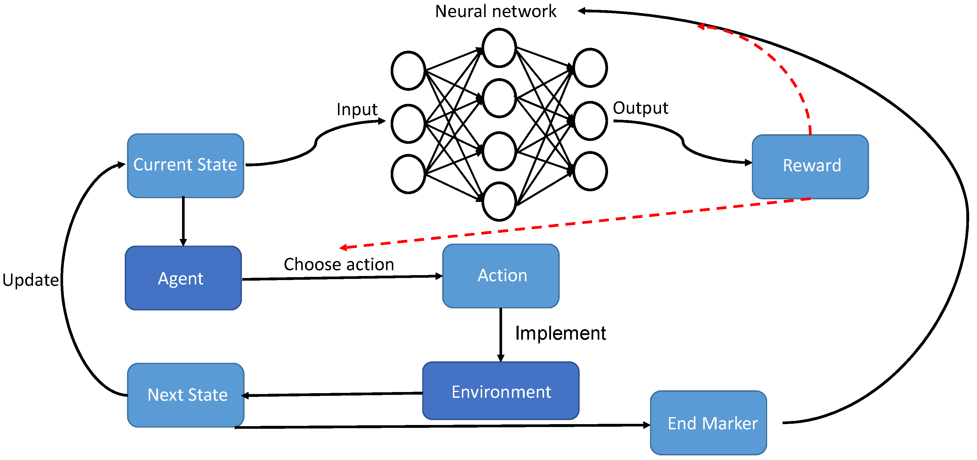
In terms of algorithmic mechanism, the policy design and transaction rules of the electricity market can be constructed as an external environment under the framework of deep reinforcement learning. The transaction behavior and electricity purchase cost of e-commerce sellers or users can be described as the action and reward function of the agent, respectively, and the state space contains some market information and physical states. By clarifying the above Markov decision information, a complete deep reinforcement learning process can be established. In terms of algorithm performance, by building a deep neural network, deep reinforcement learning does not need to perform discrete operations on continuous space, and it has sufficient ability to deal with difficult to accurately model or computationally complex problems. Therefore, it can provide new ideas for the optimization of behavior strategies of power market participants. The schematic diagram of the specific deep reinforcement learning is shown in
Figure 1.
- (1)
Environment: It is the basic environment in which the agent is located. The environment represents that the overall rules will not change, and the entire action change will be limited to the environment.
- (2)
State: It is the state of the agent in the current environment, which can also be called the characteristics of the current environment.
- (3)
Action: It is a set of all actions that the agent may take in the current environment state.
- (4)
Reward: It is the reward function. When an agent performs an action, it will acquire the value of the action in the environment, which can also be called a reward. When the action has a good, desired effect, it will acquire a higher reward, and it is hoped that the agent can continue with this action. On the contrary, when the action does not achieve the desired effect, there will be a lower reward or negative reward, and it is hoped that the agent will not perform this action later.
- (5)
Neural network: Neuron is the basic structure of neural network. a complete neuron consists of linear part and nonlinear part. The linear part is composed of input , weight , and bias , and the nonlinear part is the activation function . The mathematical expression of the neuron is as follows: .
The process steps are as follows: First, the agent generates an action strategy function (essentially the behavior or action probability distribution selected by the agent at the moment) according to the current market environment state. Then the agent performs the corresponding action,the environment generates a new clearing price and generator revenue according to the received actions and corresponding rules, and the market environment state is transferred from to . At the same time, in the above transfer process, the market environment returns the corresponding returns (excitation signal (positive, negative)) of various agents based on the definition of the objective function. Under the incentive of reward, the agent continuously adjusts its own action strategy function to optimize the mapping relationship between states and actions. The above decision-reward-optimization process is repeated continuously, so as to gradually maximize its own return or realize the optimal allocation of market resources, until the agent learns the optimal or near-optimal action strategy to maximize the return of stakeholders.
3.2. Detailed Explanation of Deep Deterministic Policy Gradient Algorithm
DDPG is an actor-criticized, model-free algorithm based on deterministic policy gradients that operates in continuous state and action spaces. The actor-critic algorithm consists of a policy function and an action-value function, the policy function acts as an actor, generating actions and interacting with the environment, the action-value function acts as a critic, evaluating the actor’s performance and guiding the actor’s follow-up. It has the following characteristics:
Approach the optimal solution by means of asymptotic strategy iteration.
Combining the deep Q network and Replay Buffer, that is, the experience return visit pool is used for state update.
Gradient update of sampling strategy using mini-batch random mini-batch samples.
On the basis of the original Actor-Critic network framework, the target network is introduced, so that the entire algorithm has 4 neural networks.
Buffer refers to a buffer space for storing sample data, and the sample buffer space is updated regularly. Actor network and Critic network extract a set small batch of samples from this buffer space each time for parameter training, and Actor network generates new strategies and environments. A new set of samples is obtained interactively, and the samples are stored in the cache space for updating, which can cancel the correlation between samples to a certain extent. In the DDPG algorithm, the Actor network is the policy network, which is used to generate the policy, and the Critic network is the value network, which is used to fit the value function and evaluate the policy generated by the Actor network. Obviously, the DDPG algorithm belongs to the off-policy type, because the Critic network is iterating and optimizing the Actor network at the same time, but the actions generated by the policy generated by the Actor network do not completely depend on the Critic network. Past practice has proved that using a single neural network algorithm, the learning process is extremely unstable, because the parameters of the network are constantly updated, and at the same time, it is used to calculate the gradient of the Actor network and the Critic network. The DDPG algorithm introduces the concept of target network, copies the original Actor and Critic networks, and copies two mirror networks. They are called the online network and the target network, respectively, so that the functions of parameter update, strategy selection/value function calculation of the network are carried out separately, so that the learning process is more stable. A schematic diagram of the principle of deep deterministic policy gradient is shown in
Figure 2.
When training a neural network, if the same neural network is used to represent the target network and the current online network, the learning process will be very unstable. Since the same network parameter needs to be used to calculate the gradient of the network while the gradient is updated frequently. DDPG has two parts, Actor and Critic. The target network and the currently updated network are two independent networks, and the entire DDPG involves a total of four neural networks: Critic target , Critic online , Actor target , Actor online .
DQN is the first method to combine deep learning with reinforcement learning. However, DQN needs to find the maximum value of the action value function in each iteration, so it can only deal with discrete, low-dimensional action spaces. There is no way for a continuous action space DQN to output the action value function for each action. A simple way to solve the above continuous action space problem is to discretize the action space, but the action space grows exponentially with the degree of freedom of the action. Deterministic Policy Gradient (DPG), which can solve the problem of continuous action space. It works by expressing the policy as a policy function
, the state
maps to a deterministic action. When the strategy is a deterministic strategy, use the Bellman equation to calculate the behavior value function
.
The optimal policy is iteratively solved by:
where
represents the update amount when updating the network
, that is,
, which is the core optimization process of the entire DDPG model. The inner layer is simply a chain rule, that is,
.
Deterministic Policy Gradient (DPG) can handle tasks in continuous action spaces but cannot directly learn policies from high-dimensional inputs; while DQN can directly learn end-to-end but can only handle discrete action spaces. Combining the two, and introducing the successful experience of the DQN algorithm on the basis of the DPG algorithm, there is a deep deterministic policy gradient algorithm (DDPG).
After training a mini-batch of data, DDPG updates the parameters of the current (online) network through the gradient ascent/gradient descent algorithm. Next, the parameters of the target network are updated by the soft update method, where the parameter is equal to
.
Use one-dimensional Gaussian noise with variance 1 as an exploration mechanism to explore the strategy set in the algorithm training process, hoping to jump out of the local optimal solution to obtain the global optimal solution. When the learning network is fully learned, the corresponding filters are added to reduce noise, so that the results of the bidding strategy tend to converge, and the final bidding strategy results are obtained. The expression for the filter method is as follows:
where
represents the number of training sessions, with the increase of training times, the threshold range of the action noise filter is
, and the noise larger than
. will be filtered out and will not participate in the neural network learning process.
The Critic network (online)
Q updates the parameter
using the TD error method in DQN, and the loss function is to minimize the mean square error:
represents the loss function of the network , the purpose is for it to fit the distance between itself and the valuation. The valuation is calculated by Equation (25). indicates that the number of samples selected from the Replay Buffer for this update is the average value. The calculation of Equation (25) uses the target Critic network and the target network as a target value, in order to make the learning process of network parameters more stable. In the beginning, this value will be very inaccurate, but gradually become more accurate as the trial progresses.
4. Algorithm Solving Process Steps
Through the above comprehensive description, combined with the market mechanism, the following variable construction process is explained:
Action: The quotation curve can best reflect the decision of a generator and has the most direct impact on the environment of the electricity market. Combined with
Section 2.3, Equation (11). This paper takes the generator’s choice of the offer curve intercept
as an action. Taking the marginal cost intercepts of all generators as the anchor criterion, the maximum value of the intercepts is set as follows:
The action space of generator is defined as: .
State: The state is used by the generator agent to describe the external environment characteristics such as quotation, load and network constraints of other generators in the electricity market. Selecting an appropriate quantity can most accurately describe the market environment faced by the agent. Define the state space for the electricity price and total load demand of each node in the network: .
Rewards: Each power generator is regarded as a rational power generator, and its income is directly used as a reward, which can be used as a direct basis.
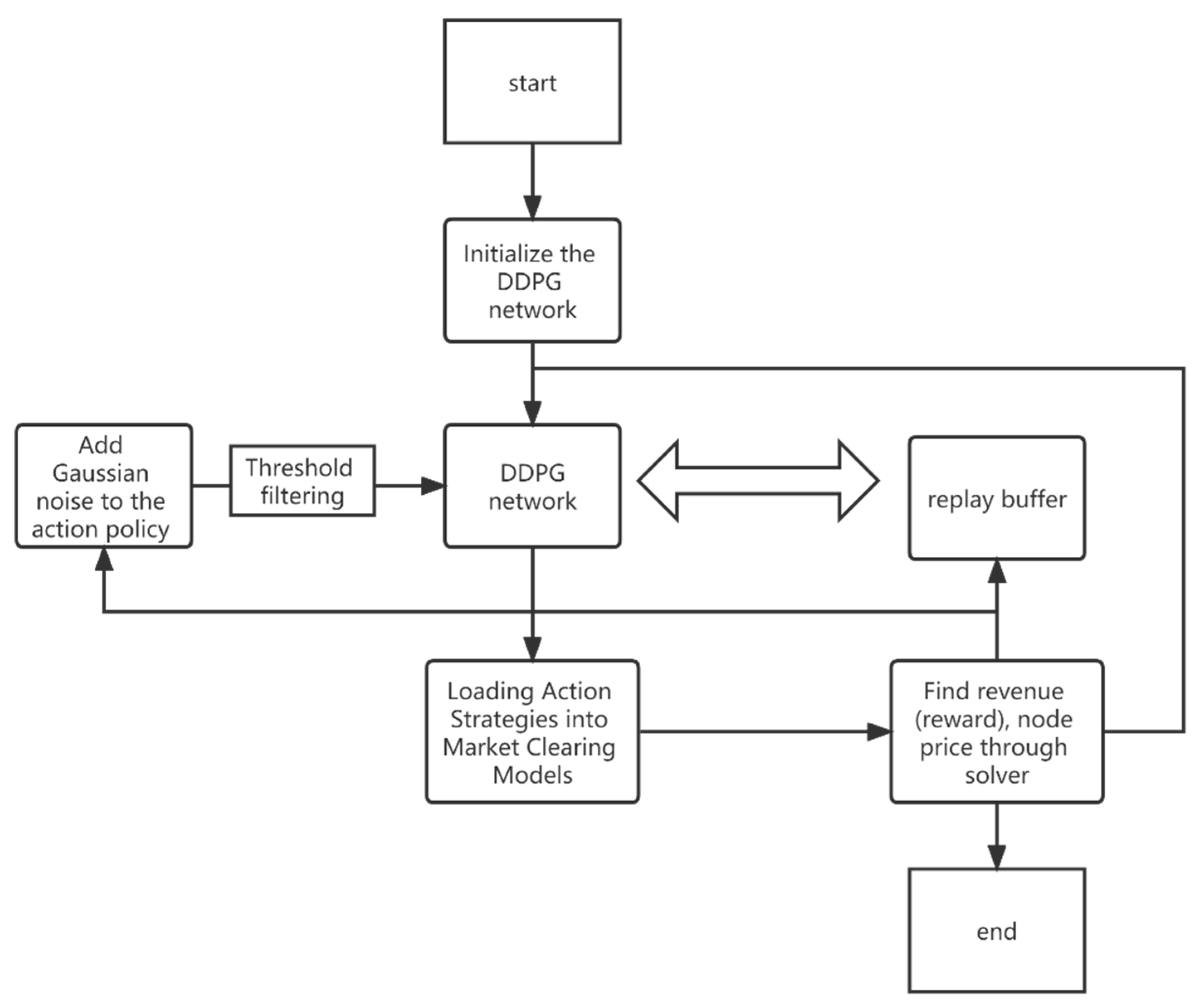
The algorithm flow execution diagram is shown in
Figure 3.
- (1)
Initialize all parameters of the network, including constructing distribution network structure parameters, generators, loads and other power transaction parameters.
- (2)
The Gaussian noise is added to the policy parameters, input into the DDPG network for calculation, and the optimal policy parameters for this round are obtained.
- (3)
The optimal parameters of this round are sent to the optimal equilibrium planning of the global linear supply function, and the market is cleared according to the maximum social welfare objective function and node power balance constraints, branch power flow out-of-limit constraints, unit output constraints, and load constraints. The revenue is returned to the DDPG network as a reward function, the node price is returned to the DDPG network as a state, and the gradient descent algorithm is used to calculate the internal network parameter values.
- (4)
The (S, A, S_, R) will be sent to the Replay buffer for parameter storage, which is convenient for DDPG network parameter update. It is continuously updated in a loop until the network parameters converge.
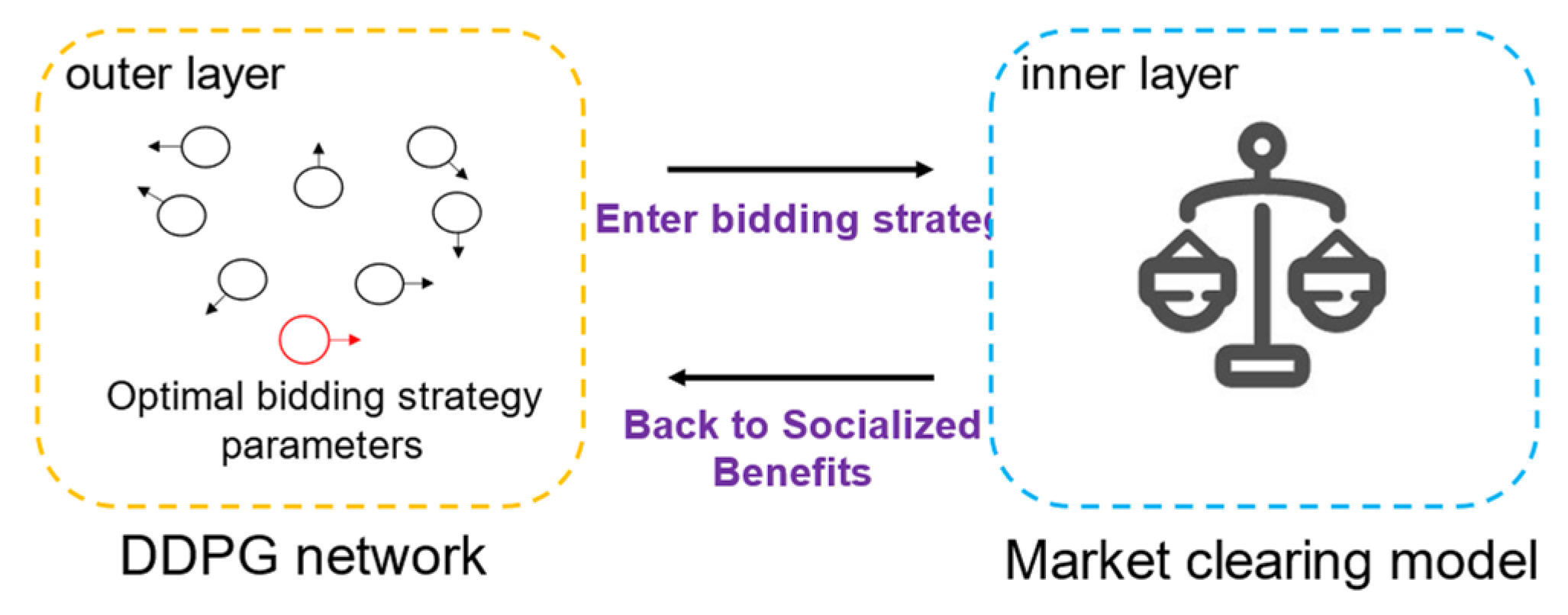
The two-layer structure of the entire algorithm is shown in
Figure 4. The inner layer is the electricity market clearing model, and the outer layer is the deep reinforcement learning algorithm. The outer layer provides bidding strategies to the inner layer, and the inner layer feeds back the revenue to the outer layer and continues to learn in a loop until the result converges and reaches the Nash equilibrium.
Electric energy production and consumption have the technical characteristics of real-time balance, and the importance and impact of market supply and demand on the electricity market are more prominent. The imbalance between power supply and demand will seriously affect market stability. An objective and comprehensive market operation efficiency evaluation index system is of great significance to the renewable energy power market. According to the main characteristics of the electricity market, the capacity bid-to-capacity ratio, which reflects system efficiency and supply-demand relationship, the transmission capacity blocking rate, which reflects regional network congestion, and the Lerner index, which reflects market power, are constructed.
The utilization of supply and demand reflects the optimal allocation of resources. Excessive adequacy means sufficient power supply and backup, indicating that the current utilization of electric power resources is insufficient, more power equipment will be idle for a long time, and the power investment efficiency is low; too low adequacy often means that Due to the shortage of power supply, this shows that the market mechanism has not effectively used price signals to guide power planning, and the market efficiency needs to be further improved. In this paper, the market efficiency indicators are expressed as follows:
when the value of
is too low, the market competitiveness is low, the supply exceeds the demand, and there is still a large capacity space in the region. When the value is too high, it means that the market competitiveness is high, the regional supply and demand relationship may change in short supply, and the spare capacity is small, so reasonable scheduling is required.
The transmission capacity blocking ratio
is used to measure the regional network congestion. This indicator reflects the local market power formed by the congestion of the transmission network, which affects the stability of the market in the blocked area. If the indicator is too high, it means that there is a serious blocking phenomenon in the system, and the market is more unstable. Therefore, it is necessary to monitor and improve the handling method and the rationality of the solution to the transmission congestion in the rules.
The Lerner index is considered to be the most direct and effective evaluation index to describe an individual in the overall market, and its evaluation characteristics indicate that it is more representative of market power itself. The unified market clearing price P in the numerator is the result of the comprehensive performance of various market factors, so this indicator evaluates individuals on the basis of integrating market factors, and is a quantitative indicator that adapts to changes in the market environment.
where
is market clearing price,
is marginal cost of a producer,
is elasticity of demand. When the value of the Lerner indicator approaches 0, it means that the supply exceeds the demand, and when it approaches 1, it means that the supply exceeds the demand.
5. Case Analysis
This section uses two different node systems to verify and analyze the proposed method, analyze whether the generator can achieve implicit collusion and policy set learning convergence under incomplete information, and use three indicators to evaluate the electricity market with renewable energy efficiency. Finally, the method is compared and verified with other four game theory methods in the electricity market.
5.1. 3-Bus System Analysis
Taking the IEEE 2-machine 3-node bus system as an example, two-layer optimization is used for policy learning. The generator parameters and load parameters are shown in
Table 1, and other power transaction parameters are shown in
Table 2.
After the output of the DDPG network, the output range of the action parameter bm of the network is −1 to 1 (the range of tanh(x)), so it needs to be scaled to the feasible range of the strategy variable. Before scaling to the strategy variable, it must be in the network. Gaussian noise and filters are added to prevent training overfitting to facilitate generalization learning of the DDPG algorithm. The following
Figure 5 shows the process of adding noise as the training changes. At the beginning, the noise is kept the maximum to ensure sufficient training. With the increase of training times, the noise will gradually decrease under the action of the filtering threshold to maintain the stability and convergence of the network.
For the convenience of presentation, sampling with a tolerance of 100 is performed according to the training sequence. The
Figure 6 shows the change of load demand with the market clearing price. When the network first started to learn, the bidding fluctuated greatly. Since the load is an elastic load, there is a relationship between the electricity price and electricity consumption that users are willing to accept.
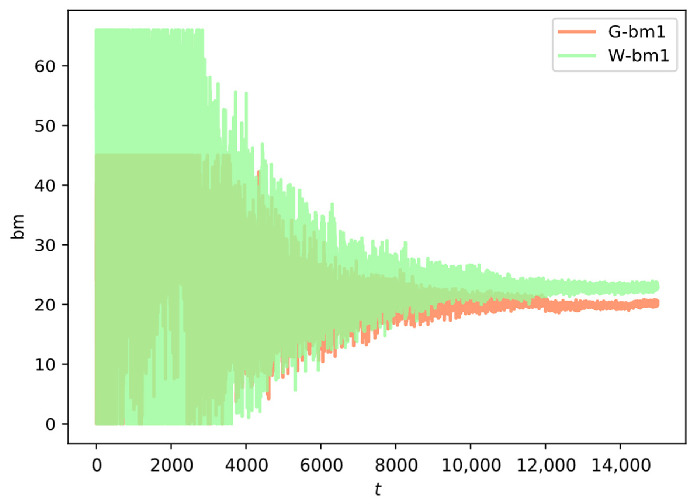
The
Figure 7 below shows the strategy convergence results after DDPG has been trained. It can be seen that at the beginning, due to the blessing of noise, the strategy fluctuated greatly. As the noise gradually diminished, the strategies of the two power generation companies also began to converge. and keep the fluctuations small. The
Figure 8 shows the income of wind power and thermal power companies in the market clearing model. From the beginning, both parties have lower returns, or only one party has higher returns. Gradually, through market tacit conspiracy and through the experimental economics by repeating the simulation, we can finally see that the Nash equilibrium is achieved, which not only achieves the role of maximizing social welfare, but also achieves a win-win situation for both parties.
The
Table 3 shows the results of other parameters. It can be seen that when wind power companies have lower costs as a renewable energy source, their Lerner index in this market is stronger than thermal power companies, and they have a higher degree of participation. This is mainly due to the consideration of the green certificate trading mechanism and the carbon market quota mechanism, which reduces the income of thermal power suppliers and increases the income of renewable energy. Although the output range of thermal power companies is larger than that of wind power companies, due to the increase of this mechanism, the competitiveness of renewable energy in the power market has been greatly improved. Compared with thermal power companies, there is a higher demand elasticity. Renewable energy has great advantages; in particular, renewable energy with green certificates and carbon emission trading mechanisms has strong market competitiveness and can obtain higher benefits through policies. In addition, market efficiency is gradually skewed towards renewable energy.
The overall efficiency of the region can also be seen from the transmission capacity blocking ratio . The low value of this indicator indicates that the current area is oversupplied, and there is no blockage that affects market stability. However, on the other hand, there is a large amount of backup energy that cannot complete the bidding, indicating that the market in this region is inefficient, and it is possible to send power or increase load consumption, which provides a basis for policy decision-making.
5.2. 30-Bus System Analysis
Similarly, referring to the above experiments, this section takes the IEEE 6-machine 30-node bus system as an example for analysis. The power generation parameters and load parameters are shown in
Table 4, and other power transaction parameters are shown in
Table 2.
The network noise curve of the IEEE 6-machine 30-node system is the same as in the previous section. Eight typical loads are selected, and the load demand function change curve is shown in
Figure 9. When prices are volatile, load demand also fluctuates. When the market clears prices and stabilizes, the load demand function fluctuates smaller.
The
Figure 10 shows the result of strategy convergence of the IEEE 6-machine 30-node system after DDPG network training. It can be seen that at the beginning, with the blessing of noise, the network fluctuates greatly. With the action of the filter, the strategy set of each generator also gradually stabilized. The
Figure 11 shows the incentive earnings for six generators. At the beginning of the training, the income of each generator fluctuates greatly. With continuous training, the revenue of each generator gradually stabilizes and reaches a relative Nash equilibrium state.
The
Figure 12 and
Figure 13 and
Table 5 shows the results for other parameters. It can be seen that after adding the green certificate trading mechanism and carbon emission trading mechanism, the Lerner index of wind power companies in the market is stronger than that of thermal power companies, the participation rate is higher, the income is higher, and the bidding volume of the maximum power is achieved. Judging from the bidding capacity ratio, renewable energy generators have strong market power and high supply and demand efficiency. From the regional point of view, the transmission capacity blocking ratio E = 0.6, which is higher than the previous 3-node network system, indicating that the market supply and demand relationship tends to be saturated, and there may be transmission congestion. On the other hand, policy regulation can be adopted to increase regional network capacity to reduce this indicator.
Section 5.1 and
Section 5.2 use the method proposed in this paper to train on a 3-node network and a 30-node network for optimal bidding strategies and maximum social welfare. In order to further evaluate the pros and cons of the algorithm proposed in this paper, the outer-layer DDPG algorithm (
Figure 4) is replaced by two types of commonly used heuristic algorithms and two types of traditional neural network algorithms for solving operations. It can be seen from
Table 6 that the two-layer algorithm proposed in this paper can achieve the Nash equilibrium of the income of each e-commerce retailer under the tacit collusion, and can also obtain greater social welfare. The comparative verification further shows that the algorithm has superiority and applicability.
6. Conclusions
This paper proposes a two-layer model of deep reinforcement learning bidding strategy for electricity market with renewable energy. The model is divided into two layers: the outer layer is the deep reinforcement learning DDPG model, and the inner layer is the secondary planning and clearing model of the electricity market. Taking wind power as an example, renewable energy has introduced a green certificate trading mechanism and a carbon emissions trading mechanism. Through the simulation of experimental economics, the optimal bidding function and bidding power, as well as the market power and market efficiency of power generators, are finally obtained. First, a bidding model for the electricity market is constructed, and the bidding function is used as a change strategy. The strategy is introduced into the DDPG network model and noise interference, and filtering are added. Next, the strategy results are returned to the electricity market clearing model through continuous learning. In the optimization training, the objective function is to maximize social welfare and satisfy constraints such as power balance, power flow overrun, unit output, and load demand. The result is returned to the DDPG network for continuous looping until the end of the convergence. The final convergence of the experimental results reaches the Nash equilibrium in game theory, which is in the best interests of all parties. Compared with other power market game theory algorithms, it is found that the strategy of this paper has advantages, which can quickly select the matching bidding curve and obtain the optimal revenue strategy. In this paper, different power market efficiency indicators are used to analyze the market efficiency of the two cases. Renewable energy generators have strong competitiveness and benefits in the power market due to the support of policies. This paper is of great significance for promoting renewable energy consumption and policy basis, and provides reference and support for bidding methods in the electricity market including renewable energy.
The algorithm proposed in this paper can be extended in these aspects:
This paper uses elastic load to simulate user demand. How to adopt a more accurate demand simulation strategy and classification method needs to be further improved.
When the area network becomes more complex, the computation time and efficiency of various learning algorithms decrease. How to improve the computational efficiency remains to be further studied. At the same time, how to simulate a more complex regional bidding situation needs to be further studied.
For the medium and long-term power trading market, auxiliary service market, capacity market and other issues can be further explored and studied.


