
A Survey on Particle Swarm Optimization for Association Rule Mining

 ,
,  and
and 
Abstract
:1. Introduction
2. Association Rule Mining
2.1. Definition of ARM
2.2. Mode Types for ARM
2.2.1. CARM
2.2.2. FARM
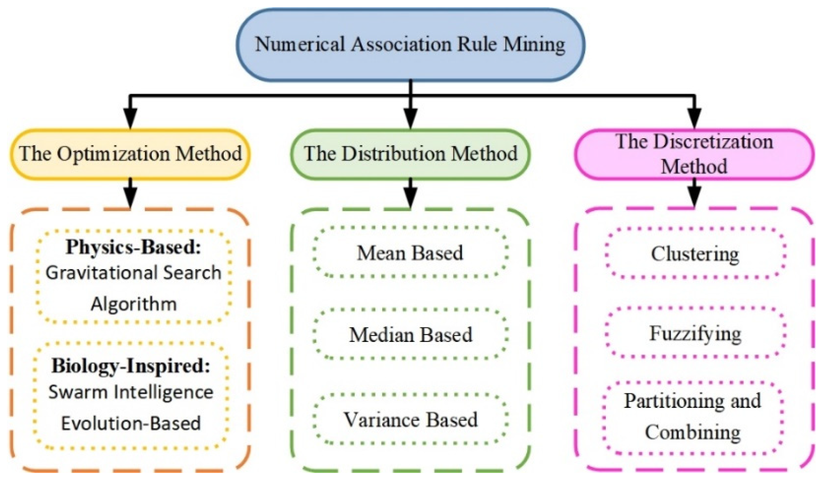
2.2.3. NARM
2.3. Evaluation Metrics for ARM
2.3.1. Basic Evaluation Indicators
2.3.2. Quantitative Evaluation Indicators
2.3.3. Qualitative Evaluation Indicators
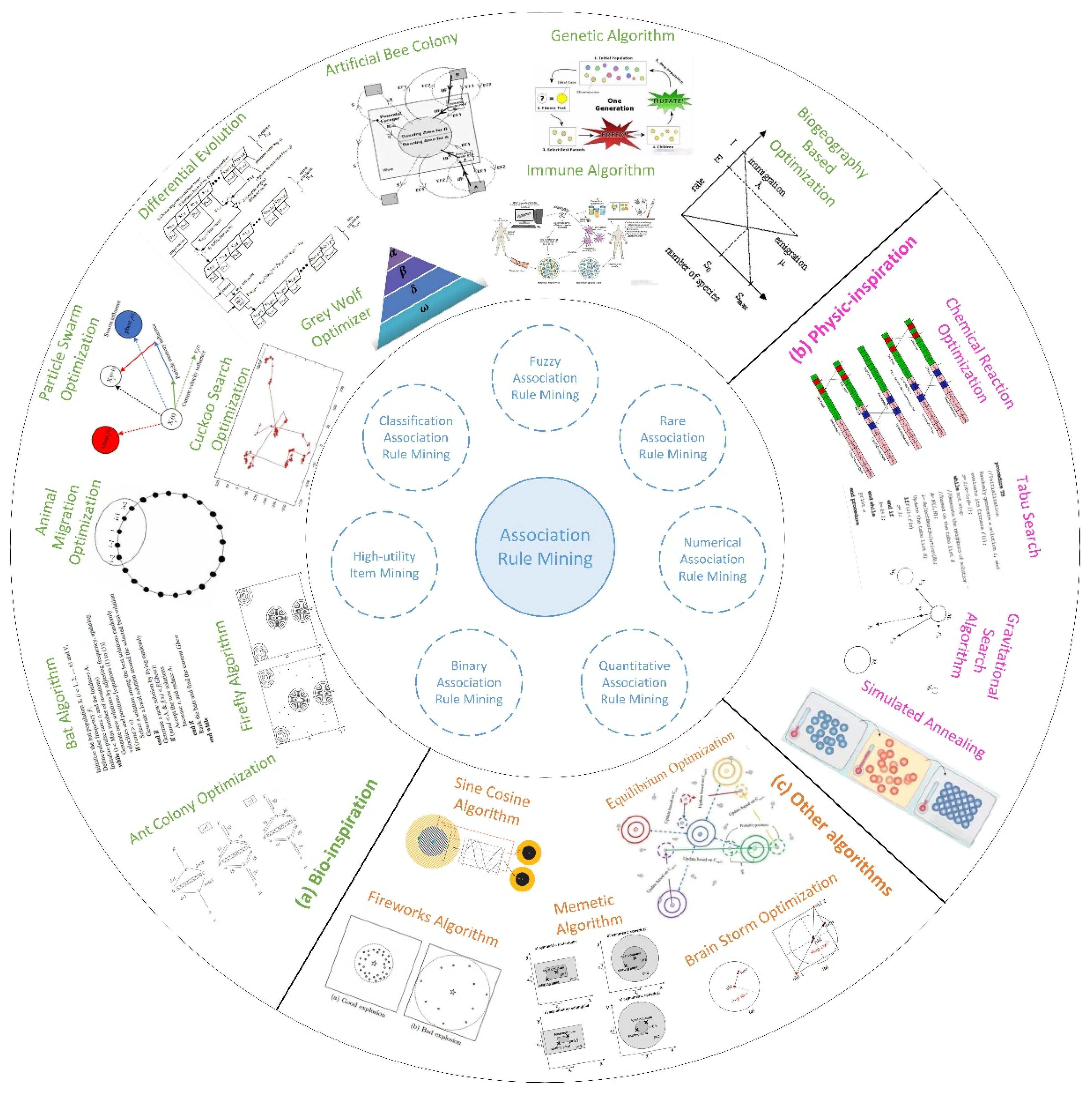
3. Comparison of Different ARM Algorithms
3.1. Bio-Inspiration
3.1.1. Evolution-Based Algorithms
3.1.2. Swarm Intelligence-Based Algorithm
3.2. Physics-Inspired
3.3. Other Algorithms
4. Particle Swarm Optimization Algorithms
4.1. Standard PSO Algorithms
| Algorithm 1 Procedure of standard PSO algorithm | |
| 1: | for each particle do |
| 2: | (a) Initialize the particle’s position and velocity. |
| 3: | (b) Evaluate the particle’s fitness value; |
| 4: | (c) Update the particle’s Pbest; |
| 5: | (d) Update the swarm’s Gbest; |
| 6: | while termination criteria is not met do |
| 7: | for each particle do |
| 8: | (a) Update particle’s velocity using Equation (12); |
| 9: | (b) Update particle’s position using Equation (13); |
| 10: | (c) Evaluate particle’s fitness value; |
| 11: | if (x[i]) < f(Pbest[i]) then |
| 12: | Update the best known position of particle i: Pbest[i]=x[i]; |
| 13: | if (Pbest[i]) < f(Gbest) then |
| 14: | Update the swarm’s best known position: Gbest=Pbest[i]; |
| 15: | (d) t = t + 1; |
| 16: | return Gbest |
4.2. Improved PSO Based on Algorithm Design
4.2.1. Swarm Initialization
4.2.2. Algorithm Parameter Optimization
4.2.3. Optimal Particle Update
4.2.4. Speed and Position Update
5. Association Rule Mining Based on PSO
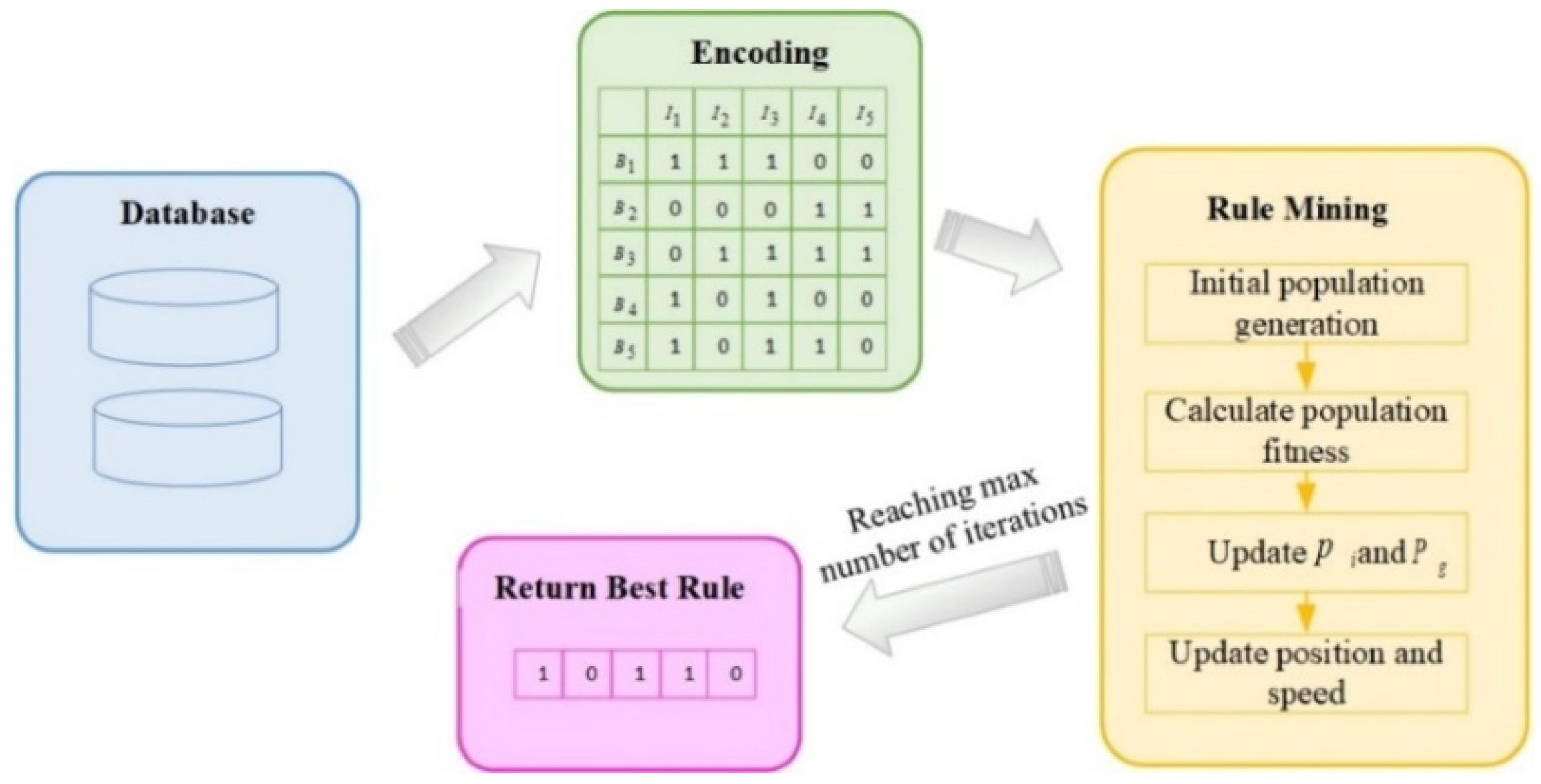
5.1. Algorithm Principle
5.1.1. ARM Process
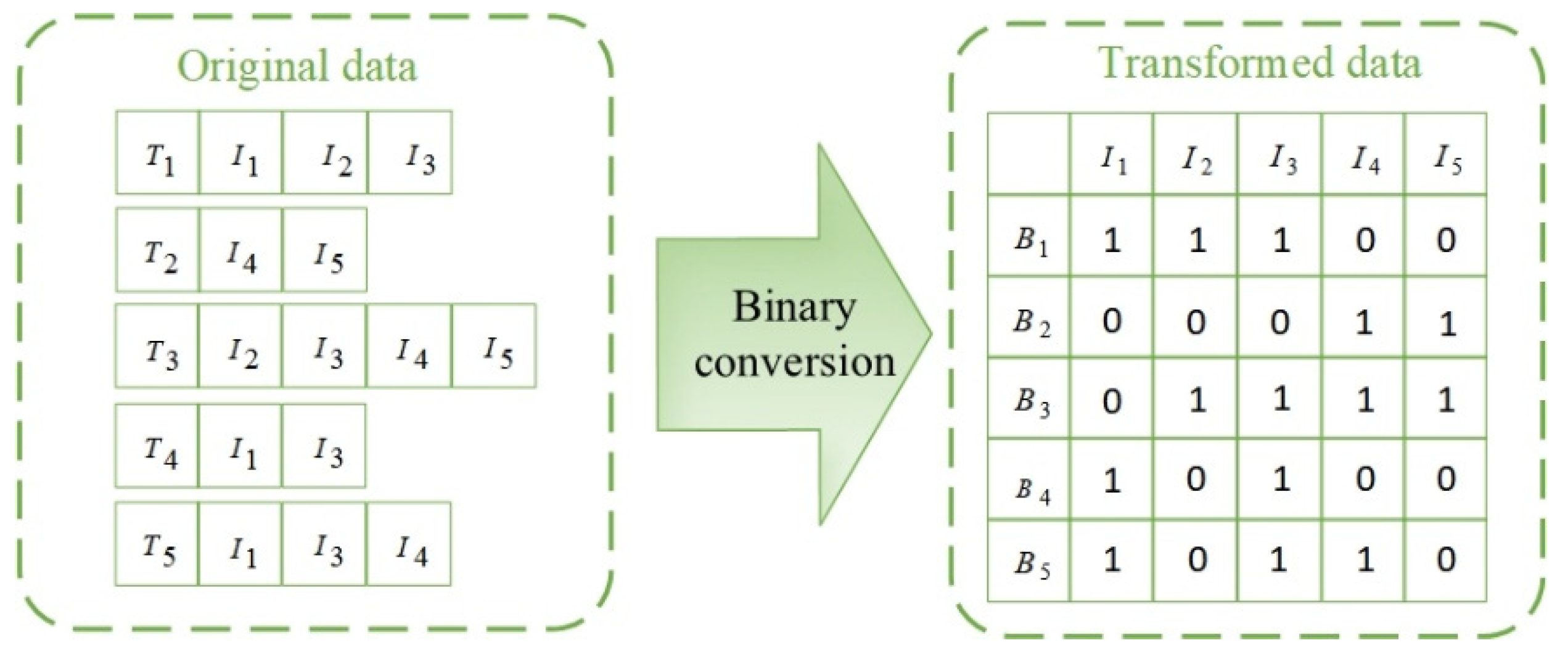
5.1.2. Binary Conversion
5.1.3. Encoding
5.1.4. Search for the Best Particle
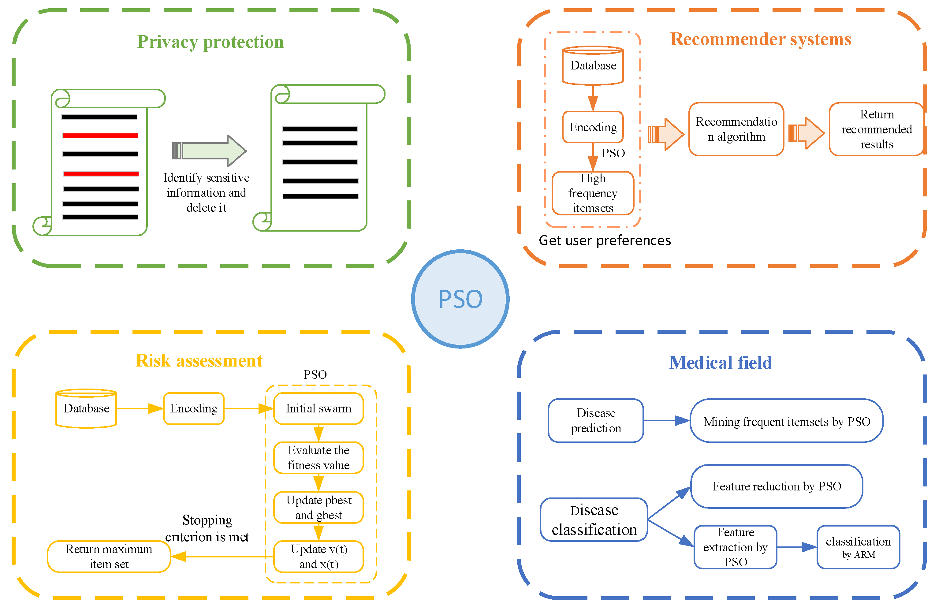
5.2. Application
5.2.1. Privacy Protection
5.2.2. Recommender Systems
5.2.3. Risk Assessment
5.2.4. Medical Field
6. Conclusions and Challenges
7. PSO Future Prospects
- (1)
- PSO algorithms converge prematurely and are prone to falling into local extremes, which mainly lie in the imbalance between global search and local search capabilities. Nevertheless, many improvement algorithms have been proposed, such as the QPSO algorithm based on the cloud model, the adaptive multi-objective PSO algorithm based on Gaussian mixed variance and elite learning, etc. However, the two are relatively contradictory, and how to dynamically maintain the balance between them in the search process to obtain the optimal solution based on the actual search results or how to measure that the two have reached the best balance needs further study.
- (2)
- Due to the exponential growth of high-dimensional data search space and low data relevance, search efficiency decreases rapidly. In addition to the existing “divide and conquer” method and the introduction of other algorithms, the use of feature extraction methods to remove redundant data and natural computational methods, such as nonlinear dimensionality reduction, can also be introduced to reduce redundancy using the maximum linear irrelevance group. Although significant progress has been made in handling large amounts of data, there is still much room for exploration in the ARM models for handling high-speed data.
- (3)
- Inertia weights and learning factors are important parameters in PSO algorithms. Improvements to inertia weights include linearly decreasing inertia weights, fuzzy inertia weights, random inertia weights, etc. Improvements in learning factors include shrinkage factors, synchronous learning factors, asynchronous learning factors, etc. In the future, we can continue to optimize these two parameters and consider whether the two affect each other and their mutual influence weights.
- (4)
- Many scholars focus more on the swarm initialization problem, including the M-class random method, fixed-value setting method, two-step method, hybrid method, etc. However, the method is too simple in how to divide the swarm size and lacks a scientific and reasonable effective division, which will limit the speed of particle movement when the swarm is too small and, thus, lead to early convergence. When the swarm is too large, it leads to a too large search space and reduces the performance and efficiency of the algorithm.
- (5)
- When there are missing or wrong datasets, there is difficulty in guaranteeing the PSO algorithm’s accuracy and performance without artificial preprocessing, i.e., having certain fault tolerance.
Author Contributions
Funding
Conflicts of Interest
References
- Agrawal, R.; Tomasz, I.; Arun, S. Mining association rules between sets of items in large databases. In Proceedings of the 1993 ACM SIGMOD International Conference on Management of Data, Washington, DC, USA, 25–28 May 1993; pp. 207–216. [Google Scholar]
- Telikani, A.; Amir, H.G.; Asadollah, S. A survey of evolutionary computation for association rule mining. Inf. Sci. 2020, 524, 318–352. [Google Scholar] [CrossRef]
- Kaushik, M.; Sharma, R.; Peious, S.A.; Shahin, M.; Yahia, S.B.; Draheim, D. A systematic assessment of numerical association rule mining methods. SN Comput. Sci. 2021, 2, 1–13. [Google Scholar] [CrossRef]
- Djenouri, Y.; Fournier, V.P.; Belhadi, A.; Chun, W.L. Metaheuristics for frequent and high-utility itemset mining. In High-Utility Pattern Mining; Springer: Berlin/Heidelberg, Germany, 2019; pp. 261–278. [Google Scholar]
- Ghobaei, A.M.; Shahidinejad, A. An efficient resource provisioning approach for analyzing cloud workloads: A metaheuristic-based clustering approach. J. Supercomput. 2021, 77, 711–750. [Google Scholar] [CrossRef]
- Gan, X.; Gong, D.; Gao, X.; Zhang, Y.; Lin, L.; Lan, T. Research on Construction of Mining Model of Association Rules for Temporal Data based on CNN. In Proceedings of the 2021 IEEE International Conference on Electronic Communications, Internet of Things and Big Data (ICEIB), Yilan County, Taiwan, 10–12 December 2021; pp. 233–235. [Google Scholar]
- Chen, S.; Xi, J.; Chen, Y.; Zhao, J. Association mining of near misses in hydropower engineering construction based on convolutional neural network text classification. Comput. Intell. Neurosci. 2022, 2022, 1–6. [Google Scholar] [CrossRef]
- He, B.; Zhang, J. An Association Rule Mining Method Based on Named Entity Recognition and Text Classification. Arab. J. Sci. Eng. 2022, 6, 1–9. [Google Scholar] [CrossRef]
- Badhon, B.; Kabir, M.M.; Xu, S.; Kabir, M. A survey on association rule mining based on evolutionary algorithms. Int. J. Comput. Appl. 2021, 43, 775–785. [Google Scholar] [CrossRef]
- Kheirollahi, H.; Chahardowli, M.; Simjoo, M. A new method of well clustering and association rule mining. J. Pet. Sci. Eng. 2022, 214, 110479. [Google Scholar] [CrossRef]
- Datta, S.; Mali, K. Significant association rule mining with high associability. In Proceedings of the IEEE 2021 5th International Conference on Intelligent Computing and Control Systems (ICICCS), Madurai, India, 6–8 May 2021; pp. 1159–1164. [Google Scholar]
- Rathee, S.; Kashyap, A. Adaptive-Miner: An efficient distributed association rule mining algorithm on Spark. J. Big Data 2018, 5, 1–17. [Google Scholar] [CrossRef]
- Zhong, Q.Y.; Qian, Q.; Feng, Y.; Fu, Y. BPSO Algorithm with Opposition-Based Learning Method for Association Rule Mining. In Advancements in Mechatronics and Intelligent Robotics; Springer: Berlin/Heidelberg, Germany, 2021; Volume 1220, pp. 351–358. [Google Scholar]
- Baró, G.B.; Martínez, T.J.F.; Rosas, R.M.V.; Ochoa, J.A.C.; González, A.Y.R.; Cortés, M.S.L. A PSO-based algorithm for mining association rules using a guided exploration strategy. Pattern Recognit. Lett. 2020, 138, 8–15. [Google Scholar] [CrossRef]
- Fister, J.I.; Fister, I. A Brief Overview of Swarm Intelligence-Based Algorithms for Numerical Association Rule Mining. Appl. Optim. Swarm Intell. 2021, 8, 47–59. [Google Scholar]
- Wang, C.; Bian, W.; Wang, R.; Chen, H.; Ye, Z.; Yan, L. Association rules mining in parallel conditional tree based on grid computing inspired partition algorithm. Int. J. Web Grid Serv. 2020, 16, 321–339. [Google Scholar] [CrossRef]
- Yuan, J. An anomaly data mining method for mass sensor networks using improved PSO algorithm based on spark parallel framework. J. Grid Comput. 2020, 18, 251–261. [Google Scholar] [CrossRef]
- Sukanya, N.S.; Thangaiah, P.R.J. Customized Particle Swarm Optimization Algorithm for Frequent Itemset Mining. In Proceedings of the IEEE 2020 International Conference on Computer Communication and Informatics (ICCCI), Coimbatore, India, 22–24 January 2020; pp. 1–4. [Google Scholar]
- Dubey, A.K.; Kumar, A.; Agrawal, R. An efficient ACO-PSO-based framework for data classification and preprocessing in big data. Evol. Intell. 2021, 14, 909–922. [Google Scholar] [CrossRef]
- Tofighy, S.; Rahmanian, A.A.; Ghobaei, A.M. An ensemble CPU load prediction algorithm using a Bayesian information criterion and smooth filters in a cloud computing environment. Softw. Pract. Exp. 2018, 48, 2257–2277. [Google Scholar] [CrossRef]
- Gad, A.G. Particle Swarm Optimization Algorithm and Its Applications: A Systematic Review. Arch. Comput. Methods Eng. 2022, 1–31. [Google Scholar]
- Nasr, M.; Hamdy, M.; Hegazy, D.; Bahnasy, K. An efficient algorithm for unique class association rule mining. Expert Syst. Appl. 2021, 164, 113978. [Google Scholar] [CrossRef]
- Kuok, C.M.; Fu, A.; Wong, M.H. Mining fuzzy association rules in databases. ACM SIGMOD Rec. 1998, 27, 41–46. [Google Scholar] [CrossRef]
- Ting, C.K.; Liaw, R.T.; Wang, T.C.; Hong, T.P. Mining fuzzy association rules using a memetic algorithm based on structure representation. Memetic Comput. 2018, 10, 15–28. [Google Scholar] [CrossRef]
- Varol, A.E.; Alatas, B. Computing, Performance analysis of multi-objective artificial intelligence optimization algorithms in numerical association rule mining. J. Ambient. Intell. Humaniz. Comput. 2020, 11, 3449–3469. [Google Scholar] [CrossRef]
- Altay, E.V.; Alatas, B. Intelligent optimization algorithms for the problem of mining numerical association rules. Phys. A Stat. Mech. Appl. 2020, 540, 123142. [Google Scholar] [CrossRef]
- Heraguemi, K.E.; Kamel, N.; Drias, H. Multi-objective bat algorithm for mining numerical association rules. Int. J. Bio-Inspired Comput. 2018, 11, 239–248. [Google Scholar] [CrossRef]
- Srikant, R.; Agrawal, R. Mining quantitative association rules in large relational tables. In Proceedings of the 1996 ACM SIGMOD International Conference on Management of Data, Montreal, QC, Canada, 4–6 June 1996; pp. 1–12. [Google Scholar]
- Song, X.D.; Zhai, K.; Gao, W. The Research of Evaulation index in Association Rules. Microcomput. Inf. 2007, 23, 174–176. [Google Scholar]
- Wang, C.; Liu, Y.; Zhang, Q.; Guo, H.; Liang, X.; Chen, Y.; Wei, Y. Association rule mining based parameter adaptive strategy for differential evolution algorithms. Expert Syst. Appl. 2019, 123, 54–69. [Google Scholar] [CrossRef]
- Altay, E.V.; Alatas, B. Differential evolution and sine cosine algorithm based novel hybrid multi-objective approaches for numerical association rule mining. Inf. Sci. 2021, 554, 198–221. [Google Scholar] [CrossRef]
- Guan, B.; Zhao, Y.; Yin, Y.; Li, Y. A differential evolution based feature combination selection algorithm for high-dimensional data. Inf. Sci. 2021, 547, 870–886. [Google Scholar] [CrossRef]
- Menaga, D.; Saravanan, S. GA-PPARM: Constraint-based objective function and genetic algorithm for privacy preserved association rule mining. Evol. Intell. 2021, 15, 1487–1498. [Google Scholar] [CrossRef]
- Lin, J.C.W.; Djenouri, Y.; Srivastava, G.; Yun, U.; Fournier-Viger, P. A predictive GA-based model for closed high-utility itemset mining. Appl. Soft Comput. 2021, 108, 107422. [Google Scholar] [CrossRef]
- Neysiani, B.S.; Soltani, N.; Mofidi, R.; NadimiShahraki, M.H. Improve performance of association rule-based collaborative filtering recommendation systems using genetic algorithm. Int. J. Inf. Technol. Comput. Sci. 2019, 11, 48–55. [Google Scholar] [CrossRef]
- Giri, P.K.; De, S.S.; Dehuri, S.; Cho, S.B. Biogeography based optimization for mining rules to assess credit risk. Intell. Syst. Account. Financ. Manag. 2021, 28, 35–51. [Google Scholar] [CrossRef]
- Ghobaei, A.M. A workload clustering based resource provisioning mechanism using Biogeography based optimization technique in the cloud based systems. Soft Comput. 2021, 25, 3813–3830. [Google Scholar] [CrossRef]
- Mo, H.; Xu, L. Immune clone algorithm for mining association rules on dynamic databases. In Proceedings of the 17th IEEE International Conference on Tools with Artificial Intelligence (ICTAI’05), Hong Kong, China, 14–16 November 2005; Volume 5, pp. 202–206. [Google Scholar]
- Husain, M.S. Exploiting Artificial Immune System to Optimize Association Rules for Word Sense Disambiguation. Int. J. Intell. Syst. Appl. Eng. 2021, 9, 184–190. [Google Scholar] [CrossRef]
- Cunha, D.S.; Castro, L.N. Evolutionary and immune algorithms applied to association rule mining in static and stream data. In Proceedings of the 2018 IEEE Congress on Evolutionary Computation (CEC), Rio de Janeiro, Brazil, 8–13 July 2018; pp. 1–8. [Google Scholar]
- Tyagi, S.; Bharadwaj, K.K. Enhancing collaborative filtering recommendations by utilizing multi-objective particle swarm optimization embedded association rule mining. Swarm Evol. Comput. 2013, 13, 1–12. [Google Scholar] [CrossRef]
- Kuo, R.J.; Gosumolo, M.; Zulvia, F.E. Multi-objective particle swarm optimization algorithm using adaptive archive grid for numerical association rule mining. Neural Comput. Appl. 2019, 31, 3559–3572. [Google Scholar] [CrossRef]
- Agarwal, A.; Nanavati, N. Association rule mining using hybrid GA-PSO for multi-objective optimisation. In Proceedings of the 2016 IEEE International Conference on Computational Intelligence and Computing Research (ICCIC), Chennai, India, 15–17 December 2016; pp. 1–7. [Google Scholar]
- Moslehi, F.; Haeri, A.; Martínez-Álvarez, F. A novel hybrid GA–PSO framework for mining quantitative association rules. Soft Comput. 2020, 24, 4645–4666. [Google Scholar] [CrossRef]
- Roopa Devi, E.M.; Suganthe, R.C. Enhanced transductive support vector machine classification with grey wolf optimizer cuckoo search optimization for intrusion detection system. Concurr. Comput. Pract. Exp. 2020, 32, e4999. [Google Scholar] [CrossRef]
- Chiclana, F.; Kumar, R.; Mittal, M.; Khari, M.; Chatterjee, J.M.; Baik, S.W. ARM–AMO: An efficient association rule mining algorithm based on animal migration optimization. Knowl. Based Syst. 2018, 154, 68–80. [Google Scholar]
- Pradeep, G.; Ravi, V.; Krishna, G.J. Hybrid Evolutionary Computing-based Association Rule Mining. In Soft Computing in Interdisciplinary Sciences; Springer: Singapore, 2022; pp. 223–243. [Google Scholar]
- Pazhaniraja, N.; Sountharrajan, S.; Sathis, K.B. High utility itemset mining: A Boolean operators-based modified grey wolf optimization algorithm. Soft Comput. 2020, 24, 16691–16704. [Google Scholar] [CrossRef]
- Yildirim, G.; Alatas, B. New adaptive intelligent grey wolf optimizer based multi-objective quantitative classification rules mining approaches. J. Ambient. Intell. Humaniz. Comput. 2021, 12, 9611–9635. [Google Scholar] [CrossRef]
- Chantar, H.; Mafarja, M.; Alsawalqah, H.; Heidari, A.A.; Aljarah, I.; Faris, H. Feature selection using binary grey wolf optimizer with elite-based crossover for Arabic text classification. Neural Comput. Appl. 2020, 32, 12201–12220. [Google Scholar] [CrossRef]
- Telikani, A.; Gandomi, A.H.; Shahbahrami, A.; Dehkordi, M.N. Privacy-preserving in association rule mining using an improved discrete binary artificial bee colony. Expert Syst. Appl. 2020, 144, 113097. [Google Scholar] [CrossRef]
- Turabieh, H.; Azwari, S.A.; Rokaya, M.; Alosaimi, W.; Alharbi, A.; Alhakami, W.; Alnfiai, M. Enhanced Harris Hawks optimization as a feature selection for the prediction of student performance. Computing 2021, 103, 1417–1438. [Google Scholar] [CrossRef]
- Dong, D.; Ye, Z.; Cao, Y.; Xie, S.; Wang, F.; Ming, W. An improved association rule mining algorithm based on ant lion optimizer algorithm and FP-growth. In Proceedings of the 2019 10th IEEE International Conference on Intelligent Data Acquisition and Advanced Computing Systems: Technology and Applications (IDAACS), Metz, France, 18–21 September 2019; Volume 1, pp. 458–463. [Google Scholar]
- Nawaz, M.S.; Fournier, V.P.; Yun, U.; Wu, Y.; Song, W. Mining high utility itemsets with hill climbing and simulated annealing. ACM Trans. Manag. Inf. Syst. (TMIS) 2021, 13, 1–22. [Google Scholar] [CrossRef]
- Ospina, M.H.; Quintana, J.L.A.; Lopez, V.F.J.; Berrio, G.S.; Barrero, L.H.; Sana, S.S. Extraction of decision rules using genetic algorithms and simulated annealing for prediction of severity of traffic accidents by motorcyclists. J. Ambient. Intell. Humaniz. Comput. 2021, 12, 10051–10072. [Google Scholar] [CrossRef]
- Chou, Y.H.; Kuo, S.Y.; Chen, C.Y.; Chao, H.C. A rule-based dynamic decision-making stock trading system based on quantum-inspired tabu search algorithm. IEEE Access 2014, 2, 883–896. [Google Scholar] [CrossRef]
- Derouiche, A.; Layeb, A.; Habbas, Z. Frequent Itemsets Mining with Chemical Reaction Optimization Metaheuristic. In Proceedings of the IEEE 2018 3rd International Conference on Pattern Analysis and Intelligent Systems (PAIS), Tebessa, Algeria, 24–25 October 2018; pp. 1–6. [Google Scholar]
- Taradeh, M.; Mafarja, M.; Heidari, A.A.; Faris, H.; Aljarah, I.; Mirjalili, S.; Fujita, H. An evolutionary gravitational search-based feature selection. Inf. Sci. 2019, 497, 219–239. [Google Scholar] [CrossRef]
- Tuba, E.; Jovanovic, R.; Hrosik, R.C.; Alihodzic, A.; Tuba, M. Web intelligence data clustering by bare bone fireworks algorithm combined with k-means. In Proceedings of the 8th International Conference on Web Intelligence, Mining and Semantics, Novi Sad, Serbia, 25–27 June 2018; pp. 1–8. [Google Scholar]
- Abualigah, L.; Dulaimi, A.J. A novel feature selection method for data mining tasks using hybrid sine cosine algorithm and genetic algorithm. Clust. Comput. 2021, 24, 2161–2176. [Google Scholar] [CrossRef]
- Djenouri, Y.; Drias, H.; Chemchem, A. A hybrid bees swarm optimization and tabu search algorithm for association rule mining. In Proceedings of the IEEE 2013 World Congress on Nature and Biologically Inspired Computing, Fargo, ND, USA, 12–14 August 2013; pp. 120–125. [Google Scholar]
- Ma, L.; Zhang, T.; Wang, R.; Yang, G.; Zhang, Y. Pbar: Parallelized brain storm optimization for association rule mining. In Proceedings of the 2019 IEEE Congress on Evolutionary Computation (CEC), Wellington, New Zealand, 10–13 June 2019; pp. 1148–1156. [Google Scholar]
- Djenouri, Y.; Djenouri, D.; Belhadi, A.; Fournier, V.P.; Lin, J.C.W.; Bendjoudi, A. Exploiting GPU parallelism in improving bees swarm optimization for mining big transactional databases. Inf. Sci. 2019, 496, 326–342. [Google Scholar] [CrossRef]
- Malik, M.M.; Haouassi, H. Efficient sequential covering strategy for classification rules mining using a discrete equilibrium optimization algorithm. J. King Saud Univ. Comput. Inf. Sci. 2021, in press. [Google Scholar] [CrossRef]
- Eberhart, R.; Kennedy, J. A new optimizer using particle swarm theory. In Proceedings of the IEEE Sixth International Symposium on Micro Machine and Human Science, MHS’95, Nagoya, Japan, 4–6 October 1995; Volume 2, pp. 39–43. [Google Scholar]
- Wang, C.W.; Yin, S.L.; Liu, W.Y.; Wei, X.M.; Zheng, H.J.; Yang, J.P. High utility itemset mining algorithm based on improved particle swarm optimization. J. Chin. Comput. Syst. 2020, 41, 1084–1090. [Google Scholar]
- Dubey, K.; Sharma, S.C. A novel multi-objective CR-PSO task scheduling algorithm with deadline constraint in cloud computing. Sustain. Comput. Inform. Syst. 2021, 32, 100605. [Google Scholar] [CrossRef]
- Hematpour, N.; Ahadpour, S. Execution examination of chaotic S-box dependent on improved PSO algorithm. Neural Comput. Appl. 2021, 33, 5111–5133. [Google Scholar] [CrossRef]
- Li, A.D.; Xue, B.; Zhang, M. Improved binary particle swarm optimization for feature selection with new initialization and search space reduction strategies. Appl. Soft Comput. 2021, 106, 107302. [Google Scholar] [CrossRef]
- Wang, S.; Yu, X.; Jia, W. A New Population Initialization of Particle Swarm Optimization Method Based on PCA for Feature Selection. J. Big Data 2021, 3, 1–9. [Google Scholar] [CrossRef]
- Bangyal, W.H.; Hameed, A.; Alosaimi, W.; Alyami, H. A new initialization approach in particle swarm optimization for global optimization problems. Comput. Intell. Neurosci. 2021, 2021, 1–17. [Google Scholar] [CrossRef]
- Pervaiz, S.; Haider, B.W.; Ashraf, A.; Nisar, K.; Haque, M.R.; Ibrahim, A.; Rawat, D.B. Comparative Research Directions of Population Initialization Techniques using PSO Algorithm. Intell. Autom. Soft Comput. 2022, 32, 1427–1444. [Google Scholar] [CrossRef]
- Tian, S.; Li, Y.; Kang, Y.; Xia, J. Multi-robot path planning in wireless sensor networks based on jump mechanism PSO and safety gap obstacle avoidance. Future Gener. Comput. Syst. 2021, 118, 37–47. [Google Scholar] [CrossRef]
- Xiang, L.I.; Chen, J. A modified PSO Algorithm based on Cloud Theory for optimizing the Fuzzy PID controller. J. Phys. Conf. Ser. 2022, 2183, 012014. [Google Scholar]
- Zhang, J.; Sheng, J.; Lu, J.; Shen, L. UCPSO: A uniform initialized particle swarm optimization algorithm with cosine inertia weight. Comput. Intell. Neurosci. 2021, 2021, 41–59. [Google Scholar] [CrossRef]
- Agrawal, A.; Tripathi, S. Particle swarm optimization with adaptive inertia weight based on cumulative binomial probability. Evol. Intell. 2021, 14, 305–313. [Google Scholar] [CrossRef]
- Komarudin, A.; Setyawan, N.; Kamajaya, L.; Achmadiah, M.N.; Zulfatman, Z. Signature PSO: A novel inertia weight adjustment using fuzzy signature for LQR tuning. Bull. Electr. Eng. Inform. 2021, 10, 308–318. [Google Scholar] [CrossRef]
- Fan, M.; Akhter, Y. A time-varying adaptive inertia weight based modified PSO algorithm for UAV path planning. In Proceedings of the IEEE 2021 2nd International Conference on Robotics, Electrical and Signal Processing Techniques (ICREST), Dhaka, Bangladesh, 5–7 January 2021; pp. 573–576. [Google Scholar]
- Chrouta, J.; Farhani, F.; Zaafouri, A. A modified multi swarm particle swarm optimization algorithm using an adaptive factor selection strategy. Trans. Inst. Meas. Control. 2021, 3, 01423312211029509. [Google Scholar] [CrossRef]
- Osei, K.J.; Han, F.; Amponsah, A.A.; Ling, Q.; Abeo, T.A. A hybrid optimization method by incorporating adaptive response strategy for Feedforward neural network. Connect. Sci. 2022, 34, 578–607. [Google Scholar] [CrossRef]
- Li, Z.; Wang, F.; Wang, R.J. An Improved Particle Swarm Optimization Algorithm. Available online: http://kns.cnki.net/kcms/detail/11.4762.TP.20210831.0841.008.html (accessed on 31 August 2021).
- Keshavamurthy, B.N. Improved PSO for task scheduling in cloud computing. In Evolution in Computational Intelligence; Springer: Singapore, 2021; pp. 467–474. [Google Scholar]
- Amponsah, A.A.; Han, F.; Osei, K.J.; Bonah, E.; Ling, Q.H. An improved multi-leader comprehensive learning particle swarm optimisation based on gravitational search algorithm. Connect. Sci. 2021, 33, 803–834. [Google Scholar] [CrossRef]
- Miao, Z.; Yong, P.; Mei, Y.; Quanjun, Y.; Xu, X. A discrete PSO-based static load balancing algorithm for distributed simulations in a cloud environment. Future Gener. Comput. Syst. 2021, 115, 497–516. [Google Scholar] [CrossRef]
- Zhu, D.; Huang, Z.; Xie, L.; Zhou, C. Improved Particle Swarm Based on Elastic Collision for DNA Coding Optimization Design. IEEE Access 2022, 10, 63592–63605. [Google Scholar] [CrossRef]
- Fu, K.; Cai, X.; Yuan, B.; Yang, Y.; Yao, X. An Efficient Surrogate Assisted Particle Swarm Optimization for Antenna Synthesis. IEEE Trans. Antennas Propag. 2022, 70, 4977–4984. [Google Scholar] [CrossRef]
- Song, B.; Wang, Z.; Zou, L. An improved PSO algorithm for smooth path planning of mobile robots using continuous high-degree Bezier curve. Appl. Soft Comput. 2021, 100, 106960. [Google Scholar] [CrossRef]
- Shaheen, M.A.M.; Hasanien, H.M.; Alkuhayli, A. A novel hybrid GWO-PSO optimization technique for optimal reactive power dispatch problem solution. Ain Shams Eng. J. 2021, 12, 621–630. [Google Scholar] [CrossRef]
- Suman, G.K.; Guerrero, J.M.; Roy, O.P. Optimisation of solar/wind/bio-generator/diesel/battery based microgrids for rural areas: A PSO-GWO approach. Sustain. Cities Soc. 2021, 67, 102723. [Google Scholar] [CrossRef]
- Xu, L.; Huang, C.; Li, C.; Wang, J.; Liu, H.; Wang, X. Estimation of tool wear and optimization of cutting parameters based on novel ANFIS-PSO method toward intelligent machining. J. Intell. Manuf. 2021, 32, 77–90. [Google Scholar] [CrossRef]
- Su, S.; Zhai, Z.; Wang, C.; Ding, K. Improved fractional-order PSO for PID tuning. Int. J. Pattern Recognit. Artif. Intell. 2021, 35, 2159016. [Google Scholar] [CrossRef]
- Zhong, Q.Y.; Qian, Q.; Fu, Y.F.; Yong, F.E.N.G. Survey of particle swarm optimization algorithm for association rule mining. J. Front. Comput. Sci. Technol. 2021, 15, 777–793. [Google Scholar]
- Kalyani, G.; Chandra, S.R.M.V.P.; Janakiramaiah, B. Particle swarm intelligence and impact factor-based privacy preserving association rule mining for balancing data utility and knowledge privacy. Arab. J. Sci. Eng. 2018, 43, 4161–4178. [Google Scholar] [CrossRef]
- Jangra, S.; Toshniwal, D. VIDPSO: Victim item deletion based PSO inspired sensitive pattern hiding algorithm for dense datasets. Inf. Process. Manag. 2020, 57, 102255. [Google Scholar] [CrossRef]
- Suma, B.; Shobha, G. Fractional salp swarm algorithm: An association rule based privacy-preserving strategy for data sanitization. J. Inf. Secur. Appl. 2022, 68, 103224. [Google Scholar]
- Krishnamoorthy, S.; Sadasivam, G.S.; Rajalakshmi, M.; Kowsalyaa, K.; Dhivya, M. Privacy preserving fuzzy association rule mining in data clusters using particle swarm optimization. Int. J. Intell. Inf. Technol. (IJIIT) 2017, 13, 1–20. [Google Scholar] [CrossRef]
- Guo, S.W.; Meng, Y.Y.; Chen, S.L. Application of improved PSOGM algorithm in dynamic association rule mining. Comput. Eng. Appl. 2018, 54, 160–165. [Google Scholar]
- Kou, Z.C. Binary particle swarm optimization-based association rule mining for machine capabilities and part features. J. Univ. Jinan Sci. Technol. 2019, 33, 381–388. [Google Scholar]
- Kaur, S.; Goyal, M. Fast and robust hybrid particle swarm optimization tabu search association rule mining (HPSO-ARM) algorithm for web data association rule mining (WDARM). Int. J. Adv. Res. Comput. Sci. Manag. Stud. 2014, 2, 448–451. [Google Scholar]
- Gangurde, R.A.; Kumar, B. Next Web Page Prediction using Genetic Algorithm and Feed Forward Association Rule based on Web-Log Features. Int. J. Perform. Eng. 2020, 16, 10–18. [Google Scholar] [CrossRef]
- Jiang, H.; Kwong, C.K.; Park, W.Y.; Yu, K.M. A multi-objective PSO approach of mining association rules for affective design based on online customer reviews. J. Eng. Des. 2018, 29, 381–403. [Google Scholar] [CrossRef]
- Lanzarini, L.; Villa, M.A.; Aquino, G.; De, G.A. Obtaining classification rules using lvqPSO. In Proceedings of the ICSI 2015: Advances in Swarm and Computational Intelligence, Beijing, China, 25–28 June 2015; Springer: Cham, Switzerland, 2015; pp. 183–193. [Google Scholar]
- Priya, S.; Selvakumar, S. PaSOFuAC: Particle Swarm Optimization Based Fuzzy Associative Classifier for Detecting Phishing Websites. Wirel. Pers. Commun. 2022, 125, 755–784. [Google Scholar] [CrossRef]
- Li, S.Y.; Zhou, L.; Liu, H. Hazard ldentification Algorithm Based on Deep Extreme Learning Machine. Comput. Sci. 2017, 44, 89–94. [Google Scholar]
- She, Y.L.; Zhou, L. Hazard ldentification Algorithm Based on Improved Online Sequential Extreme Learning Machine. Comput. Technol. Dev. 2018, 28, 72–77. [Google Scholar]
- Ripon, S.; Sarowar, G.; Qasim, F.; Cynthia, S.T. An Efficient Classification of Tuberous Sclerosis Disease Using Nature Inspired PSO and ACO Based Optimized Neural Network. In Nature Inspired Computing for Data Science; Springer: Cham, Switzerland, 2020; pp. 1–28. [Google Scholar]
- Choubey, D.K.; Kumar, P.; Tripathi, S.; Kumar, S. Performance evaluation of classification methods with PCA and PSO for diabetes. Netw. Model. Anal. Health Inform. Bioinform. 2020, 9, 1–30. [Google Scholar] [CrossRef]
- Karsidani, S.D.; Farhadian, M.; Mahjub, H.; Mozayanimonfared, A. Prediction of Major Adverse Cardiovascular Events (MACCE) Following Percutaneous Coronary Intervention Using ANFIS-PSO Model. BMC Cardiovasc. Disord. 2022, 22, 389. [Google Scholar]
- Mangat, V.; Vig, R. Novel associative classifier based on dynamic adaptive PSO: Application to determining candidates for thoracic surgery. Expert Syst. Appl. 2014, 41, 8234–8244. [Google Scholar] [CrossRef]
- Raja, J.B.; Pandian, S.C. PSO-FCM based data mining model to predict diabetic disease. Comput. Methods Programs Biomed. 2020, 196, 105659. [Google Scholar] [CrossRef]
- Alkeshuosh, A.H.; Moghadam, M.Z.; Al, M.I.; Abdar, M. Using PSO algorithm for producing best rules in diagnosis of heart disease. In Proceedings of the IEEE 2017 International Conference on Computer and Applications (ICCA), Doha, United Arab Emirates, 6–7 September 2017; pp. 306–311. [Google Scholar]
- Mao, J.; Wang, H.Y. Association rule optimization for detection algorithm of factors inducing heart disease. Control. Eng. China 2017, 24, 1286–1290. [Google Scholar]
- Shao, P.; Wu, Z.; Peng, H.; Wang, Y.; Li, G. An Adaptive Particle Swarm Optimization Using Hybrid Strategy. In Proceedings of the International Symposium on Intelligence Computation and Applications, Guangzhou, China, 20–21 November 2021; Springer: Singapore, 2017; pp. 26–39. [Google Scholar]
- Liang, B.; Zhao, Y.; Li, Y. A hybrid particle swarm optimization with crisscross learning strategy. Eng. Appl. Artif. Intell. 2021, 105, 104418. [Google Scholar] [CrossRef]
- Rostami, M.; Forouzandeh, S.; Berahmand, K.; Soltani, M. Integration of multi-objective PSO based feature selection and node centrality for medical datasets. Genomics 2020, 112, 4370–4384. [Google Scholar] [CrossRef] [PubMed]
- Zhong, Q.Y.; Qian, Q.; Fu, Y.F. Association rule mining based on multi-strategy BPSO algorithm. Bull. Sci. Technol. 2021, 37, 40–46. [Google Scholar]
- Dai, Y.B. Multi-Objective Particle Swarm Algorithm Based on Quasi-Circular Mapping. Appl. Res. Comput. 2021, 38, 3673–3677. [Google Scholar]


| Algorithms | Authors | Technology | Advantages | Disadvantages |
|---|---|---|---|---|
| DE | Wang et al. [30] | Adaptive adjustment F and Cr | Enhanced algorithmic global search capability | High memory overhead |
| Altay et al. [31] | DE-SCA, Multi-target, | Performs well on datasets with few attributes and many instances | High algorithmic complexity | |
| Guan et al. [32] | HGDE | Increased swarm diversity and high stability | Unable to handle high-dimensional data items | |
| GA | Menaga et al. [33] | GAPPARM | High practicality | Easy to cause data loss |
| Lin et al. [34] | Clustering the data | High accuracy and performance | Single objective | |
| Neysiani et al. [35] | Identify similarity between itemsets by association rules | High-quality rules | Long execution time | |
| BBO | Giri et al. [36] | LGBBO-RuleMiner | High accuracy and a simple algorithm | Only for single target problems |
| Arani et al. [37] | K-means, Bayesian learning | Reduce the delay, SLA violation ratio, cost, and energy consumption | High CPU usage | |
| CSA | Mo et al. [38] | DMARICA | Short execution time, Highly scalable | Less integrity of generation rules |
| AIS | Husain et al. [39] | CLONALG | High accuracy | Accuracy is positively correlated with the number of iterations |
| Danilo et al. [40] | CLONALG-GA | Performs better in sparse datasets | Not suitable for dense datasets |
| Algorithms | Authors | Technology | Advantages | Disadvantages |
|---|---|---|---|---|
| PSO | Tyagi et al. [41] | Multi-target, MOPSO-ARM | Performs well on sparse data | Calculated overload, low efficiency |
| Kuo et al. [42] | Adaptive Archive Grid, MOPSO | Automatically finds the best interval between datasets; no data preprocessing is required. | Fewer targets to consider | |
| Baro et al. [14] | Guided search strategy | High-quality rules and short calculation times | Lower average fitness values | |
| Agarwal et al. [43] | Multi-objective | Balancing global and local search capabilities | Not applicable to quantitative association rules | |
| Moslehi et al. [44] | GA-PSO | No predefined minimum support and confidence levels are required | Generate redundant rules | |
| CSO | Devi et al. [45] | HGWCSO-ETSVM, Min-Max | High accuracy and precision | Reduced overall system performance |
| AMO | Son et al. [46] | ARM-AMO | Reduces the time and memory required for frequent itemset generation | Lower quality rules |
| BAT | Kamel et al. [27] | MSBARM, loop strategy | Rule quality is higher than other ways algorithm | Unable to handle large databases |
| FA | Pradeep et al. [47] | BFFO-TA, Feature Selection | No redundant rules are created | Not applicable to multi-objective problems |
| GWO | Pazhaniraa et al. [48] | BGWO-HUI | Low time complexity | High memory overhead |
| Yildirim et al. [49] | Adaptive multi-target intelligent search, MOGWO | For discrete, quantitative, and mixed datasets with high comprehensibility | Not suitable for distributed datasets | |
| Chantar et al. [50] | SVM, Elite Cross, BGWO | High accuracy | High time complexity | |
| ABC | Akbar et al. [51] | ABC4ARH | Highly efficient and stable | Less scalability and higher complexity |
| HHO | Turabieh et al. [52] | HHO-KNN | Enhanced ability to think outside the local optimum | Less stability |
| ALO | Dong et al. [53] | ALO-ARM | The optimized search process has high efficiency | Not suitable for large datasets |
| Algorithms | Authors | Technology | Advantages | Disadvantages |
|---|---|---|---|---|
| SA | Nawaz et al. [54] | HUIM-SA | HUIM-SA varies linearly with the number of iterations | Lack of mutation mechanisms |
| Holman et al. [55] | GA-SA, Confusion Matrix | High accuracy | Accuracy depends on dataset size | |
| TS | Chou et al. [56] | QTS | Obtain more rules | Algorithm performance degrades when the dataset is too small |
| CRO | Abir et al. [57] | CRO | Low algorithm complexity; no need to specify minimum support | Less stability, calculated overload |
| GSA | Taradeh et al. [58] | HGSA, Crossover, variation | Fast convergence and high-quality rules | Not applicable to mixed datasets |
| Algorithms | Authors | Technology | Advantages | Disadvantages |
|---|---|---|---|---|
| FA | Eva et al. [59] | Combining k-means for web data clustering | Faster convergence; better performance at the minimum distance; shorter computation time | The placement strategy of the initial center of mass needs to be further optimized |
| MA | Ting et al. [24] | Optimizing the affiliation function in FARM | Improve the search capability of the algorithm and obtain high fuzzy support | Less scalability |
| SCA | Laith et al. [60] | SCAGA | Maximum classification accuracy with minimal attributes | The imbalance between global search capability and local search capability |
| BSO | Djenouris et al. [61] | HBSO-TS | Short execution time | Poor results in large datasets |
| Ma et al. [62] | PLBSO | Parallelized processing with low computational costs | Less performance when dealing with quantitative rules | |
| Youcef et al. [63] | GBSO-Miner | Adaptable to large text and graphical databases | Thread divergence exists | |
| EO | Malik et al. [64] | DEOA-CRM | High-quality rules and highly interpretable algorithms | Poor performance in some datasets |
| Objective | Thesis |
|---|---|
| Convergence | [66,67,73,75,79,80,82,83,86,87,91,113] |
| Versatility | [66,68,73,81,83,84,87,90,113,114,115,116,117] |
| High-dimensional data | [70,71,72,115,116,117] |
| Result accuracy | [46,73,81,84,116,117] |
| Balance exploration and utilization | [67,69,74,77,78,80,82,85,86,114] |
Publisher’s Note: MDPI stays neutral with regard to jurisdictional claims in published maps and institutional affiliations. |
© 2022 by the authors. Licensee MDPI, Basel, Switzerland. This article is an open access article distributed under the terms and conditions of the Creative Commons Attribution (CC BY) license (https://creativecommons.org/licenses/by/4.0/).
Share and Cite
Li, G.; Wang, T.; Chen, Q.; Shao, P.; Xiong, N.; Vasilakos, A. A Survey on Particle Swarm Optimization for Association Rule Mining. Electronics 2022, 11, 3044. https://doi.org/10.3390/electronics11193044
Li G, Wang T, Chen Q, Shao P, Xiong N, Vasilakos A. A Survey on Particle Swarm Optimization for Association Rule Mining. Electronics. 2022; 11(19):3044. https://doi.org/10.3390/electronics11193044
Chicago/Turabian StyleLi, Guangquan, Ting Wang, Qi Chen, Peng Shao, Naixue Xiong, and Athanasios Vasilakos. 2022. "A Survey on Particle Swarm Optimization for Association Rule Mining" Electronics 11, no. 19: 3044. https://doi.org/10.3390/electronics11193044
APA StyleLi, G., Wang, T., Chen, Q., Shao, P., Xiong, N., & Vasilakos, A. (2022). A Survey on Particle Swarm Optimization for Association Rule Mining. Electronics, 11(19), 3044. https://doi.org/10.3390/electronics11193044