Multi-Class Pixel Certainty Active Learning Model for Classification of Land Cover Classes Using Hyperspectral Imagery

Abstract

An accurate identification of objects from the acquisition system depends on the clear segmentation and classification of remote sensing images. With the limited financial resources and the high intra-class variations, the earlier proposed algorithms failed to handle the sub-optimal dataset. The building of an efficient training set iteratively in active learning (AL) approaches improves classification performance. The heuristics-based AL provides better results with the inheritance of contextual information and the robustness to noise variations. The uncertainty exists pixel variations make the heuristics-based AL fail to handle the remote sensing image classification. Previously, we focused on the extraction of clear textural pattern information by using the extended differential pattern-based relevance vector machine (EDP-AL). This paper extends that work into the novel pixel-certainty activity learning (PCAL) based on the information about textural patterns obtained from the extended differential pattern (EDP). Initially, distributed intensity filtering (DIF) is used to eliminate noise from the image, and then histogram equalization (HE) is used to improve the image quality. The EDP is used to merge and classify different labels for each image sample, and this algorithm expresses the textural information. The PCAL technique is used to classify the HSI patterns that are important in remote sensing applications using this pattern collection. Pavia University and Indian Pines (IP) are the datasets used to validate the performance of the proposed PCAL (PU). The ability of PCAL to accurately categorize land cover types is demonstrated by a comparison of the proposed PCAL with existing algorithms in terms of classification accuracy and the Kappa coefficient.

1. Introduction

The accurate discrimination of an object of interest (land cover classes) depends on the clear spectral information and spatial resolution of the sensors used remotely. The real-time remote sensing image systems provide a large set of images corresponding to the various fields such as hydrological, geological, precision agriculture [1,2], ecological and military applications. Among them, the estimation of bio-mass, bio-diversity, and the changes in the land cover through hyperspectral images (HSI) is an attractive research area in ecological science [3,4]. Spectral dimensionality and the need for specific spectral-spatial classifiers are the major challenges in the HSI during the last decade. The increase in internal class variability due to the spatial variability of spectral signatures makes the HSI a challenging problem. A review of statistical learning theory (SLT) [5], based on HSI classification methods, suggests that specific loss functions and the regularization parameters are to be designed to handle the HSI classification against the spatial homogeneity variations. The developed classifiers should meet the following constraints.

• Robustness to the changes in image representation;
• Absence or a small amount of differences in classifiers during the manipulation of objects and pixels.

The design of an adequate classification model can produce accurate results within reasonable time and cost. Recently, the automatic classification techniques based on the supervised learning approach require a set of labeled reference samples for the training process. For each time the input image is to be classified, new training samples are required, which leads to cost and additional constraints. To overcome these issues, active learning (AL) is applied to create an effective and efficient training set. The periodical update of the land cover image is also a major issue in the geographical area with large size images. To overcome such issues, assumptions such as the remote sensing images and the related labeled sample from previous analysis are made. The classification of new geographical images with the same land-cover classes and similar characteristics is regarded as the domain adaption (DA) problem. The inclusion of spatial/temporal variability of the spectral signatures addresses the DA problems effectively [6]. The maximization of discrimination capabilities not only depends on the solution to DA but also depends on the cost of the labeling process. The powerful strategy in the AL is a margin-sampling-based support vector machine (SVM) [7] that describes the importance of samples based on the distance to the hyperplane. The distance metric describes the pixel uncertainty and its importance for classification.

The selection of important samples for the labeling of images of the multi-source environment is largely affected by pixel uncertainty. Most of the uncertainty measures [8] are effective due to the capture of the relationship among the candidate instances and the classification model. They do not consider the data distribution information in unlabeled data, which leads to few usage instances for labeling. Hence, the query selection process in the AL model includes the adaptive combination of uncertainty and information density. This combination provides the probabilistic weight to the class instances that minimizes the expected classification error. The assumption to perform such probabilistic weight-based AL data is homogeneous throughout the image. Due to the coverage of small regions in the image, the shift between the distributions of training samples and classification is verified. When this model is used for classification, the incompatibility of the model is to be optimized [9]. The spatial adaptation of heuristics requires contextual information: so far, the heuristics AL includes the positional information and textures. The robustness of the noise based on the uncertainty of the pixels is a major issue in the AL approaches. Hence, this paper proposed pixel-certainty active learning (PCAL) to overcome the issues in the traditional approaches. The technical contributions of the proposed PCAL are listed as follows:

• The use of distributed intensity filtering (DIF) and histogram equalization (HE) reduces noise and improves image quality [10], ensuring the accuracy of pixels.
• The fusion and classification of labels under the merging of spectrum bands are supported by an extended differential pattern (EDP) dependent texture patterns extraction.
• The utilization of PCAL on the EDP-based features provided the labeled output corresponding to the cluster index value. This facilitates the inclusion of contextual and positional information and improves the robustness of the noise variations in pixels.

The following is a breakdown of the paper’s structure: In Section 2, a full overview of related works on heuristic active learning models in spectral-spatial domains is given. Section 3 describes the pixel-certainty active learning (PCAL) implementation process. In Section 4, there is a comparison of PCAL with existing approaches. Finally, in Section 5, the conclusions about the use of PCAL to remotely sensed data are presented.

2. Related Work

The availability of rich information in HSI provides a significant chance to identify and classify the materials in the images. The inheritance of the high-number of channels with the few training samples leads to the curse of the dimensionality problem. The improvement of classification accuracy depends on the removal of noise bands generated. Jia et al. [11] proposed a new strategy to select the bands automatically without a manual removal technique. The wavelet shrinkage and the affinity propagation are applied to select the most representative bands to reduce the dimensionality. The spectroscopic analysis plays a major role in the identification of materials from the high-resolution images. Accurate estimation of classification performance depends on the unmixing strategy. Bioucas-Dias et al. [9,12] presented a brief overview of unmixing methods such as signal sub-space, geometrical, statistical, sparsity-based, and spatial-contextual unmixing with the mathematical solutions and experimental results. The integration of spatial and spectral information is a necessary task in HSI analysis. Dopido et al. [13] developed the new unmixing-based feature extraction technique that integrated the spectral and spatial information by combining the clustering with the partial spectral unmixing. They studied conditional correlations between the multiple sparse representations of different spatial neighborhood pixels. Srinivas et al. [14] proposed the probabilistic graphical method for explicitly mining conditional dependencies between the distinct sparse features. The remote sensing image classification by using the morphological profiles (MP)-based tools was alternate research to improve the classification performance. Huang et al. [15] discussed the strategies involved in the construction of morphological profiles such as linear, non-linear, manifold-learning, and multi-linear transformation-based methods. The hyper dimensional feature space was considered by using the decision function and sparse classifier.

The difference between the reflectance and the shading of objects from a single image. In the intrinsic image decomposition (IID) model, the spectral reflectance and shading component were the major factors to improve the classification performance. Kang et al. [16] proposed the novel feature extraction technique based on the IID model to reduce the spectral dimension and estimate the reflectance/shading components in the HSI classification. Li et al. [17] developed the framework to classify the hyperspectral scenes by pursuing the combination of multiple features. The major objective of mixing models was to investigate the linear and non-linear class boundaries for HSI interpretation. The utilization of multiple features improves the classification performance effectively. However, the increase in feature dimensionality induced the limitations in kernel-based classification. Liu et al. [18] provide the simultaneous learning of class-specific features that enforced the automatic learning of the sparsity in either group or feature level. By using this simultaneous way of learning, the relevant features were retained for classification. However, the high dimensional data with few labeled samples were the major difficulty in such a sparsity approach. Ul-Haq [19] exploited the certain special properties of the HSI through sparse representation models. In addition, the Homotopy-based sparse classification was proposed to prove the sparsity against the time and computational limitations. The learning of sparse-spectral representation required the spatial smoothness of the pixels to lie within the same region. Zhang et al. [20] exploited the fixed neighbor system that enforced the neighboring pixels to share the common sparsity information. The development of kernel-based group sparse coding (GSC) with the incorporation of kernel tricks to capture the non-linear relationships.

The combination of seasonal data into the spectral data faced major issues such as reduction in dimensionality and the selection of most informative samples. Rodriguez-Galiano et al. [21] used the pseudo cross and cross variograms to incorporate the seasonal/temporal information with the sparsity models. Further, the random forest (RF) [22] classifier was used to reduce the subset of input variables with better classification accuracy. Xia et al. [23] extended the RF approach into the integration of the rotation forest with the Markov random field (MRF) to model the contextual information as the maximum a posteriori problem. The adaptation of a supervised classifier depends on the trained image to the classification of other similar images. Persello et al. [24] discussed the domain adaptation (DA) problems through the AL approaches in which there is the iterative labeling and adding of the labeled samples to the set which contains the most informative samples. With the inclusion of limited resources and the human expert, the selection of samples utilizes the pool-based AL approaches in [25,26], respectively. The generalization capability of training samples from the high-dimensionality input was the recent attractive research in remote sensing applications. The SVM [27] and the wavelet domain-based multi-view learning AL [28,29] reduce the redundancy within the contention pool.

The abundant spectral information and the high dimensionality are the major challenges in conventional HSI processing. Cui et al. [30] presented the tabu search optimization technique to reduce the dimensionality of the features and developed the Compactness-Separation Coefficient (CS Coefficient) to calculate the optimal feature reduction number. The application of traditional AL classifiers such as support vector machine (SVM) and the relevant vector machine (RVM) on the reduced features yielded high classification accuracy. The minimal reconstruction error is used to determine the class label of the test pixel. To achieve this, the sparse representation classifier (SRC) based on the joint sparsity model is constructed. Zhang et al. [31] reviewed the conventional SVM and SRC-based models (joint sparse representation classifier (JSRC)) with the differential morphological profile (DMP)-based features. The review in terms of classification accuracy conveyed that the preservation of spatial information and the utilization of complementary information was achieved effectively. Due to the dimensionality of the features, the prediction of optimal features from the diverse features was the research issue in HSI classification. Feature fusion and the composite kernels support the optimal feature selection. Chunsen et al. [32] discussed the issues in the traditional vector stacking (VS)-based SVM and proposed the minimum noise fraction (MNF)-based feature extraction technique for a single feature. The information in HSI is fully utilized to compute the marginal probability estimation. Li et al. [33] discussed the marginal probability estimation model called maximum a posteriori marginal (MPM) with the loop belief propagation (LBP) algorithm. They discussed the issues in the logistic regression via splitting and augmented Lagrangian (LORSAL) and the integration of LORSAL with multi-level logistic (MILL). The comparison between the MPM-LBP with the exiting methods suggested the effectiveness of MPM-LBP methods in HSI applications. The addition of similar samples to the training dataset provides the enrichment of the semi-supervised classification process. Ayerdi and Romayin [34] proposed anticipative hybrid extreme rotation forest (AHERF) that defines the rank-based selection of probability distribution. The utilization of clustering and maximization of class spatial compactness removes the classification errors significantly. Wan et al. [35] proposed collaborative active and semi-supervised learning (CASSL), which combines AL and SSL to improve learning performance when compared to “multiclass level uncertainty-enhanced cluster-based diversity” (MCLU-ECBD) [36], “locally linear embedding with manifold Co-Regularization” (LLE-mCR) [37], and CASSL-no pseudo label verification (NoPLV). In recent studies, adequate learning with decreased time consumption was identified as a research topic in the HSI categorization. Sun et al. [38] discussed the Gaussian process (GP)-Al method, including GP-Random Selection (RS), GP-Init, GP-full, GP-AL1, GP-AL3, and GP-AL2 heuristics, among others. The above listed methods were based on heuristic approaches where the inclusion of contextual information and the robustness to the noise variations (pixel uncertainty) were the major issues. To overcome such issues, the PCAL method is proposed in this paper with the clear extracted texture patterns and the enhanced image quality. Other work conducted in [39,40,41,42,43] highlighted several GIS applications of GIS in the area of crop disease identification and mitigation strategies. Finally, mixture learning models were applied with success to solve such problems [44].

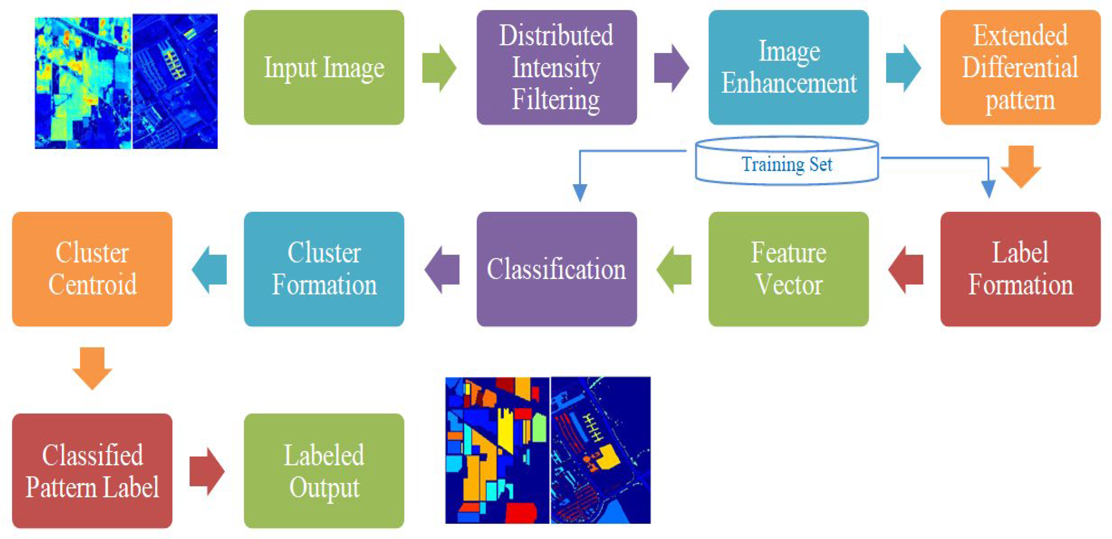
3. Pixel Certainty Active Learning

The implementation details of the proposed pixel-certainty active learning (PCAL) for distant sensing applications are discussed in this section. The proposed study relies on the following models, as illustrated in Figure 1, to accomplish simultaneous development of huge training samples and superior categorization.

• Distributed intensity filtering (DIF);
• Extended differential pattern (EDP);
• Pixel-certainty active learning (PCAL).

Figure 1. Workflow of proposed PCAL.

Figure 1. Workflow of proposed PCAL.

Low-quality images that contain noise have an impact on the depth information. The depth information is critical for hyperspectral image classification. Initially, noise in the images is removed by distributed intensity filtering (DIF), and the integration of histogram equalization (HE) improves the image quality for clear depth information analysis. The extraction of texture pattern information is then a key stage in the proposed study. The extended differential pattern (EDP) approach collects the necessary texture patterns that add significantly to the analysis’ relevant information. The PCAL is utilized with the retrieved pattern set to categorize the samples based on the clustered index values that are required for processing of optical data processing. The accuracy of the proposed PCAL model is demonstrated by comparing it to existing models on several accuracy criteria such as Kappa coefficient, false rejection rate (FRR), false acceptance rate (FAR), and genuine acceptance rate (GAR).

3.1. Distributed Intensity Filtering

The noise in the input image, as illustrated in Figure 2, has an impact on the quality of edge information, resulting in misclassification and limiting the relevant information prediction. The input image is projected into a window with a size of 3 × 3 to remove the noise contained in the image. The image projection window is shown in Figure 3.

The distributed intensity filtering (DIF) method is developed for removing image noise. The following are the primary procedures involved in this filtering:

• Locating the neighborhood about the point to be examined.
• Using the center value, examine the pixel intensities of the neighborhood.
• Substitute the analyzed result from the previous step for the original pixel value.

The image’s window is initially generated with row values ranging from I − 1 to i + 1 and column values ranging from j − 1 to j + 1. The neighborhood then moves over each pixel in the image one at a time, predicting the replacement value. The difference between the center pixel and the boundary is first calculated, then the difference value is compared to the center pixel to see if it is greater. If the condition is met, replace the pixel value with the window element’s average value as follows:

$$I_p\left(i,j\right)=\frac{\sum W_{temp}}{n}$$

(1)

where $I_p\left(i,j\right)$= Preprocessed image

$$W_{temp}=(W\left(x\right),{ }^{\prime }{x}^{\prime }\ne center)$$

$n$ = Total number of neighborhoods.

The noise in the image is reduced when the neighborhood values are replaced with the estimated value. As a result, the DIF process’ output has reduced noise, as seen in Figure 4. The interpretation of information contained in an image is not just dependent on the image’s noise-free portions. The image quality is improved even more for clear image analysis. To improve the quality of the input image, Gaussian modeling is used. In the classic Gaussian model [45], the standard deviation is reconstructed as the root mean square (RMS) value of the difference between every pixel and the total pixel value, as shown below:

$$\sigma =\sqrt{\frac{1}{a\ast b}{\displaystyle \sum }_{i=1}^{a\ast b}{\left(I_p\left(i\right)-\frac{\sum I_p}{a}\right)}^2}$$

(2)

Here, a is the row size and b is the column size of the images.

To obtain a good quality image (as Figure 5) the subsequent processing:pixel values of the actual input image are normalized with the maximal mean values from the enhanced image.

With the updated standard deviations from Equation (2), the image quality is improved as follows by Equation (3).

$$I_e=\frac{I_p}{max\left(I_p\left(\frac{\sum I_p}{a}*\sigma \right)\right)}$$

(3)

3.2. Extended Differential Pattern

The window size is increased to 5 × 5 in this stage to allow for the display of an enhanced image. The median value of the projected image is then calculated. The window over the enlarged image is initially generated with a size of 5 × 5. The cells with 3 × 3 size are retrieved independently within this window. The rules required for vector prediction are developed by using angle-based difference estimation. This section contains the algorithm for computing patterns in multi-angular form.

The amount of the difference between the window formations (temp, temp1) is stated numerically as follows by Equation (4):

$$mag=\sqrt{\left(double\left(\begin{array}{c}\left({\left(temp\left( i,j+1\right) temp\left( i,j\right)\right)}^2\right)+\left({\left(temp\left( i-1,j\right) temp\left( i,j\right)\right)}^2\right)\end{array}\right)\right)}$$

(4)

where initial $i=3$ and $j=3$.

To extract the patterns, a comparison between the center pixels and nearby pixels is conducted, followed by decimal coding. The multiplication is performed using two different types of patterns (Pt2, Pt1) to retrieve the required patterns. These relevant patterns have a significant impact on classification, as shown in Figure 6.

Algorithm 1. Extended Differential Pattern

Input: Enhanced Image ‘$I_e$’ Output: Texture pattern ‘$out$’ S-1: Initialize the 5 × 5 window matrix S-2: Project window over the enhanced image ($I_e$) For ($i=3$ to row_size-2)        For (j = 3 to Column_size-2)$temp=I_e\left(i^2+j^2\right)$ S-3: Compute the median value for the window $$med1=temp\left(j\right)$$ S-4: Check the difference between the center of the pixelwith the neighborhood If$temp$ (, i−1,j)>= $med1$&&$temp$ (i−1,j+1) ≥ $med1$ $I_{gc}$(1) = 1;           Else if $temp$ (i−1,j)<$med1$&&$temp$(i−1,j+1) ≥ $med1$ $I_{gc}$(2) = 2;           Else if $temp$ (i−1,j)<$med1$&&$temp$ (i−1,j+1) <$med1$ $I_{gc}$(3) = 3;           Else if $temp$(i−1,j)>= $med1$&&$temp$ (i−1,j+1) <$med1$ $I_{gc}$(4) = 4;           End if S-5: Compute the magnitude value from the newlyformed window by using Equation (4) S-6: Compute the patterns $Pt1=mag\times I_{gc}$ S-7: For (𝑖=2 to (𝑅𝑜𝑤_𝑠𝑖𝑧𝑒)−1) For (𝑗=2 to (𝐶𝑜𝑙𝑢𝑚𝑛_𝑠𝑖𝑧𝑒)−1) Assign the original image to the temporary variable $$temp1=I_e\left(i,j\right);$$ S-8: Check the condition $$temp2\left(i-1,j-1\right)=I_e\left(i-1,j-1\right)>temp1;$$ S-9: Compute the patterns $$Pt2=temp2$$ End Loop j End Loop i S-10: Perform the bitwise OR operation between two patterns $$out=Pt1\ast Pt2$$

3.3. Active Learning

Active learning is the process of learning with a customized program to gain control over the many inputs required for training. The main goal of such systems is to perform selected input queries against a large number of classifiers. When compared to random sampling, sample selection utilizing active learning (AL) [46] is more discriminative. The suggested work is based on the presence of a zone of uncertainty among a collection of training samples. In the repetitive training stage, the samples available are more likely to be identified wrongly. The following are the primary steps in the active learning framework: the manual labeling of positive and negative samples used in training is referred to as passive learning.

The queries are derived from the outputs generated by utilizing passive trained classifiers to manually determine true and false positives.

The AL decreases false detection rates while retaining a high detection rate. Consider the $X={\left(x_i,y_i\right)}_{i=1}^l$ list of labeled samples that mapped into the input space χ of dimension (d). Furthermore, unlabeled samples are considered to be part of the $U={\left(x_i\right)}_{i=l+1}^{l+u}$ the pool of candidates. The performance of the classification model is improved by feeding it with fresh tagged pixels on a regular basis. The following are the algorithmic steps for classical AL.

1. For each iteration, initialize the training sets and pool of candidates, as well as the number of pixels provided to the classification model.

2. Use the present training set to train a model.

3. For every candidate in the candidate pool, compute the user-defined heuristic.

4. Each contender is given a rank based on the heuristic score.

5. Choose the most intriguing pixels based on the rank values.

6. Set the label to the pixels you have chosen.

7. Include the batch in the practice set.

8. Remove that batch of candidates from running.

The communication between the user and the model is a key prerequisite for active learning. The primary requirement for an AL training system is the availability of labeled material with class-knowledge and the interpretive outcomes of distributed classes. The relevant pixels are required to complete the execution, which is a critical task in the traditional framework. In addition, the ranking of pixels follows the heuristic process that leads to difficulty in labeling against the practical conditions such as illumination, and pose variations. Then, the lack of clear information on texture patterns provided misguided results in existing methods. The inclusion of contextual information in the heuristics requires both spectral and positional information for the learning algorithm. The robustness to noise is the crucial issue that is based on the uncertainty that leads to useless heuristics in existing methods. To alleviate these issues, pixel-certainty active learning (PCAL) model is proposed in this paper. The employment of DIF and EDP in the proposed work removes the noise level in the image and extracts the detailed texture patterns, respectively. These patterns are applied to the PCAL to obtain the labeled output image effectively.

Pixel-Certainty Active Learning

The proposed algorithm receives the inputs from the feature extraction block and produces the labeled output from the cluster-based heuristic process. The parameters used in PCAL are illustrated in

Table 1. PCAL Parameters.

S.No	Variable	Parameter
1	α	Distance Function
2	β	Accumulation Array
3	$\theta$	Total Sum Distance
4	$\omega$	Index
5	λ	Best Total Sum Distance
6	$\vartheta$	Summed
7	μ	Best Summed
8	$N$	Emptyerror

.

In the proposed work, the pool of candidates is regarded as the pattern outputs from the feature extraction block. The user defined heuristic values are distance function, index, and accumulation array. The sequential processes for the proposed PCAL algorithm are listed as follows:

PCAL Algorithm

Input: Image Pattern Output: Clustering Output (C) Step_1: Initialize the cluster for output (C) and the variable (m) to store the minimum index Step_2: Select the sample from the patterns Step_3: Compute the d distance among samples Step_4: Extract minimum index score correspond to minimum distance ω = min (d) Step_5: Construct the array() for minimum index, distance values $$\partial =\beta$$ Step_6: Add the sample corresponding to the minimum index or distance value $$\theta =\sum \left(\vartheta \right)$$ Step_7: If $\theta <\lambda$ Step_8: Replace the index with the best index ω and best = ω. Step_9: Update the distance, index and cluster values Step_10: Update the Distance function by using the following equation $$d=(D\left(i\right)+X\left(j\right)-C{\left(i,j\right)}^2), \mathrm{i} \mathrm{Row}, \mathrm{and} \mathrm{j} \mathrm{Column}$$ Step_11: Extract the clustered output with the updated centroid value (C)

The labeled output from the clustered index and the corresponding labeled image is shown in Figure 7 and Figure 8, respectively. From Figure 8, it is observed that the labels are assigned to the different classes of input images from Indian Pines (IP) and Pavia University (PU). There are 16 and 9 classes available in IP and PU datasets. The proposed algorithm assigned the labels to each class effectively with detailed information.

4. Performance Analysis

This subsection depicts the proposed PCAL’s performance analysis in terms of recall, precision, specificity, and sensitivity. In hyperspectral image analysis, the suggested PCAL was compared to the current SVM [30], class level joint sparse representation classifier (CL-JSRC) [31], probabilistic weighed strategy [32], and EDP-AL.

Dataset: To validate the performance of the proposed PCAL, two datasets were used: Indian Pines hyperspectral datasets and Pavia University [47]. The reflective optics spectrographic imaging system (ROSIS) sensor, which has 610 × 340 pixels and 103 spectral bands ranging from 0.43 to 0.86 μm, was used to acquire the Pavia University dataset. It has a spatial resolution of 1.3 m. The AVIRIS sensor collects the Indian Pines dataset. With 220 spectral bands ranging from 0.4 to 2.5 μm and a spatial resolution of 20 m, the dataset includes 145 × 145 pixels.

Table 2. Number of labeled samples and information classes (Pavia University).

Class	Train	Test
Asphalt	310	6206
Meadows	806	16,123
Gravel	94	1880
Trees	146	2933
Metal	67	1345
Bare Soil	251	5029
Bitumen	66	1330
Bricks	184	3682
Shadow	47	947
Total	1971	39,475

and

Table 3. Number of labelled samples and information classes (Indian Pines).

Class	Train	Test
Oats	10	20
Grass-mowed	13	26
Alfalfa	27	54
Bldg-grass-drives	50	380
Corn	50	234
Corn-Min	50	834
Corn-notill	50	1434
Grass/Pasture	50	497
Grass/Trees	50	747
Hay-windrowed	50	489
Soybeans-clean	50	614
Soybeans-Min	50	2468
Soybeans-notill	50	968
Stone-steel-towers	50	95
Wheat	50	212
Woods	50	1294
Total	700	10,366

list the information classes and labeled samples for Indian Pines and Pavian University.

4.1. Classification Accuracy and Kappa Coefficient Analysis

The suggested PCAL was compared to the SVM-DMP [26,31], approaches that were already in use.

Table 4. Accuracy and Kappa Coefficient Analysis (Indian Pines).

CLASS	SVM-DMP [31]	SRC-DMP [31]	JSRC-DMP [31]	Raw [32]	MNF [32]	VS-SVM [32]	EDP-AL	PCAL
1	82.75	83.14	85.1	82.93	68.85	100	97.92	97.6
2	83.48	87.85	90.92	60.66	73.99	94.26	97.8	99.6
3	87.83	89.18	86.74	41.07	53.99	91.39	99.96	100
4	91.35	88.92	87.34	31.82	55.76	82.65	99.96	99.92
5	92.22	93.41	91.36	59.13	80.39	96.77	100	99.76
6	96.11	94.36	92.98	88.29	96.3	99.59	100	100
7	92.5	97.08	81.67	96.3	100	100	100	99.96
8	97.16	97.13	95.54	97.1	99.35	100	99.96	99.44
9	51.58	56.32	48.95	63.64	100	100	100	100
10	71.64	83.48	86.83	61.32	61.83	88.54	100	99.72
11	90.22	90.51	96.17	78.29	83.24	97.42	100	100
12	73.46	78.78	79.78	45.29	56.86	97.93	100	99.84
13	97.61	97.91	98.61	88.44	97.14	99.66	100	100
14	97.99	98.19	98.9	89.99	93.34	100	100	99.8
15	94.93	96.45	88.53	56.28	70.36	94.88	100	99.76
16	78.11	79.56	74.67	98.89	95.7	97.84	100	99.96
Kappa Coeff	86.65	89.21	90.71	62.5	72.92	95.16	96.42	97.1

and

Table 5. Accuracy and Kappa Coefficient Analysis (Pavia University).

CLASS	SVM-DMP [31]	SRC-DMP [31]	JSRC-DMP [31]	RAW [32]	MNF [32]	VS-SVM [32]	EDP-AL	PCAL
1	93.77	84.41	87.95	81.99	84.86	92.12	99.68	98.2
2	97.35	97.09	97.89	94.22	84.5	99.56	98.4	100
3	65.04	56.76	61.9	68.11	74.32	85.65	98.72	99.48
4	93.7	90.64	93.75	79.92	75.06	98.24	97.97	99.52
5	72.91	83.9	89.9	97.94	99.55	99.7	97.49	99.84
6	81.84	64.12	71.66	65.43	78.58	94.43	97.01	99.68
7	65.28	75.05	77.43	67.85	82.72	90.45	96.53	100
8	89.35	72.21	79.21	67.79	78.9	92.34	96.05	100
9	69.03	84.02	89.21	100	100	100	95.57	100
Kappa Coeff	86.7	80.28	84.65	76.76	77.89	94.72	95.87	97.72

indicate the differences in accuracy rate (for every class of the dataset) and Kappa coefficient for JSRC-DMP, Raw, NMF, and VS-SVM [32].

When compared to other approaches, the JSRC-DMP and VS-SVM offered improved classification accuracy and kappa coefficient for each image class. However, in the suggested work, the differential pattern extracts relevant patterns from a variety of patterns, improving the accuracy rate and coefficient value even more.

4.2. Acceptance/Rejection Rate Analysis

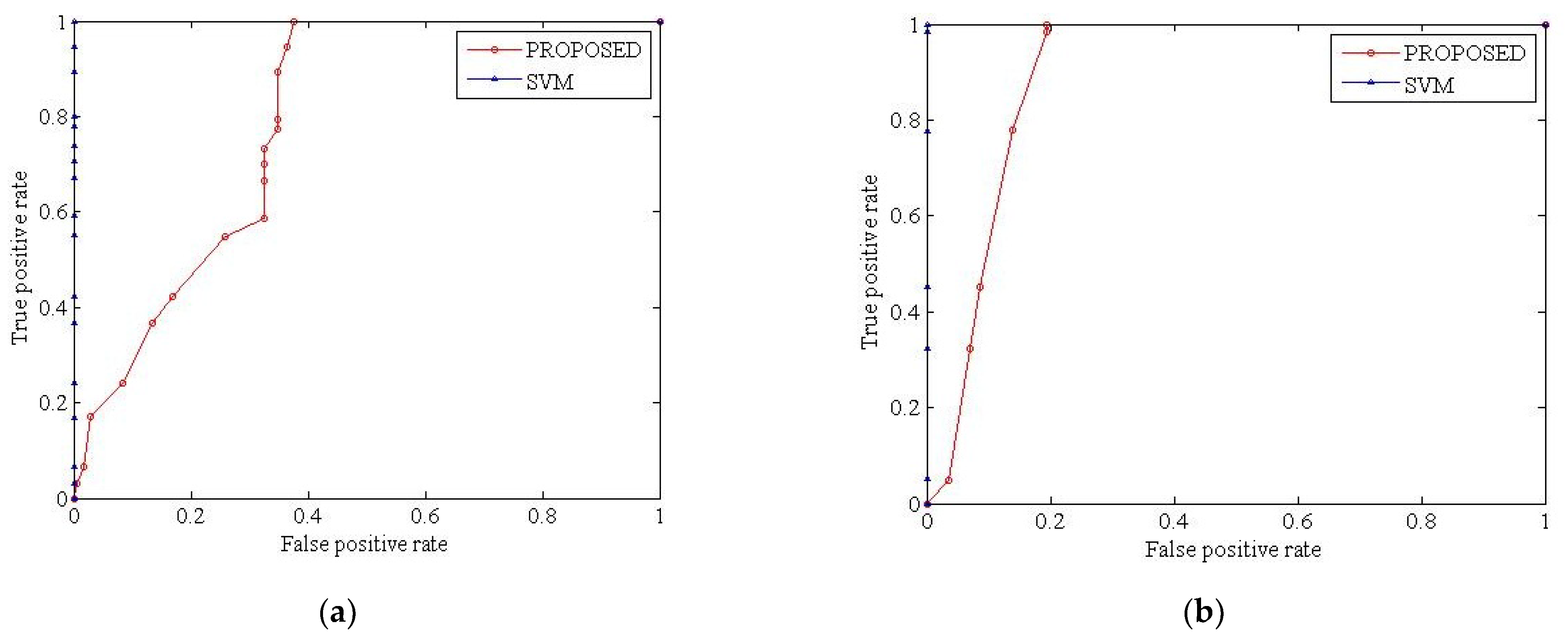
Two measures called false acceptance rate (FAR) and false rejection rate (FRR) define the number of inaccurate labeling for each unauthorized user attempt and the rejection. The following are the mathematical formulas for facial expression recognition: FAR, FRR, and genuine acceptance rate (GAR) Equations (5)–(7):

$$FAR=\left(Falseclaimsacceptance\right)/\left(Totalclaims\right)\times 100$$

(5)

$$FRR=\left(Falseclaimsrejection\right)/\left(Totalclaims\right)\times 100$$

(6)

$$GAR=100-FAR$$

(7)

The analysis of FAR, FRR, and GAR for the randomly selected two image classes from the dataset is depicted in Figure 9, Figure 10 and Figure 11, respectively, for the PU and IP datasets. The comparison of PCAL (proposed) and the existing SVM states that the FAR and GAR values for the proposed PCAL are better than the existing SVM approaches.

For image classes 1 and 2, the FAR values of the existing SVM are high and low for the proposed PCAL. The inclusion of differential patterns and the PCAL based methods improved the acceptance rate performance effectively.

4.3. ROC Analysis

The fundamental metric to validate the performance of the testing process in learning is called receiver operating characteristics, which is the variation of the true positive rate (TPR) against the false positive rate (FPR). The mathematical formulations of TPR by Equation (8) and FPR (Equation (9)) are described as follows:

$$TruePositiveRate=\frac{Numberofcorrectlyclassifiedsamples}{Totalnumberofsamples}$$

(8)

$$\begin{gathered} FalsePositiveRate=1-specificity= \\ 1-\frac{Numberofincrrectlyclassifiedsamples}{Totalnumberofsamples} \end{gathered}$$

(9)

The ROC performance study of the proposed PCAL with the existing SVM for IP and PU datasets is shown in Figure 12a,b. Due to the differential-based texture pattern and low dimensionality, the suggested PCAL provides a high true positivity rate for small values of false positive rate, as shown in Figure 12a,b.

4.4. Overall Accuracy Analysis

The variations of overall classification accuracy for the existing MPM-LPM, LORSAL-MILL, LORSAL, SVM [33], and AHERF [34] with different training percentages as shown in

Table 6. Overall accuracy.

METHODOLOGY (Percentage Training for IP and PU)	Overall Accuracy
	INDIAN PINES (IP)	PAVIA UNIVERSITY (PU)
MPM-LMP [33] 10.00% (IP), 0.68%(PU)	94.76	85.78
AHERF [34] 2.50% (IP), 3.00% (PU)	93.67	98.09
LORSAL-MILL [33] 10.00% (IP), 0.68% (PU)	92.72	85.57
AHERF [34] 3.00% (IP), 2.50% (PU)	93.58	97.17
LORSAL [33] 10.00% (IP), 0.68% (PU)	82.6	85.42
SVM [33] 10.00% (IP), 0.68%	80.56	80.99
AHERF [34] 1.50% (IP), 0.50% (PU)	87.93	87.81
PCAL	97.6	98.48

.

In existing methods, the AHERF provides better results for IP and PU datasets compared to other methods. However, the proper noise removal and improvement of robustness of the pixels to noise variations in the proposed PCAL improves the classification accuracy to 97.6 and 98.48% compared to AHERF. The hybrid EDP and the pixel-certainty-based AL improves the classification performance of HSI in remote sensing applications.

4.5. Accuracy Analysis with Existing AL Approaches

The suggested EDP-AL and known approaches of MCLU-ECBD [36], CASSL-NoPLV, CASSL [35], and LLE-mCR [37] were used to compare AA (average accuracy). Furthermore, a comparison of the suggested EDP-AA, AL’s OA (overall accuracy), and Kappa coefficient with the existing GP-based AL versions [38] suggests that the proposed PCAL is useful in remote sensing applications.

The following is the mathematical formulation of the Kappa coefficient (in percent) Equation (10),

$$Kappa Coefficient(\%)=\frac{OA-AA}{100-A}$$

(10)

On the PU and IP, Figure 13 depicts the differences in OA, AA, and Kappa statistics for proposed and existing AL techniques. The suggested PCAL has an AA of 94.31 percent, which is higher than existing approaches. Similarly, EDP-OA, AL’s AA, and Kappa statistics are 96.31, 57.93, and 91.22 percent, respectively, which are higher than the current EDP-AL technique.

5. Conclusions

Through the use of a combination of differential texture-pattern extraction and PCAL, this paper addressed the limits in HSI classification and suggested framework remedies. The uncertainty exists pixel variations made the heuristics-based AL a failure to handle the remote sensing image classification. Previously, we focused on the extraction of clear textural pattern information by using the extended differential pattern-based relevance vector machine (EDP-AL) [1]. Based on the textural pattern information collected from the EDP, this research extended that work into the PCAL. Initially, the DIF eliminated the image’s noise, and the addition of HE improved the image’s quality. The EDP performed the merging and categorization of distinct labels for each image sample, clearly displaying the textural information. The PCAL technique is used to classify the HSI patterns that are important in remote sensing applications using this pattern collection. The usefulness of PCAL in remote sensing applications was demonstrated by a comparison of the proposed PCAL with existing AL algorithms in terms of classification accuracy and Kappa coefficient.

References

1. Pradhan, S.R.M.K.; Sinha, B.L. Extended differential pattern-based large scale live active learning model for classification of remote sensing data. Int. J. Chem. Stud. 2019, 7, 1610–1620. [Google Scholar]
2. Haq, M.A. Intellligent sustainable agricultural water practice using multi sensor spatiotemporal evolution. Environ. Technol. 2021, 1–14. [Google Scholar] [CrossRef] [PubMed]
3. Benediktsson, J.A.; Chanussot, J.; Moon, W.M. Very High-Resolution Remote Sensing: Challenges and Opportunities [Point of View]. Proc. IEEE 2012, 100, 1907–1910. [Google Scholar] [CrossRef]
4. Camps-Valls, G.; Tuia, D.; Bruzzone, L.; Benediktsson, J.A. Advances in Hyperspectral Image Classification: Earth Monitoring with Statistical Learning Methods. IEEE Signal Process. Mag. 2014, 31, 45–54. [Google Scholar] [CrossRef]
5. Fauvel, M.; Tarabalka, Y.; Benediktsson, J.A.; Chanussot, J.; Tilton, J.C. Advances in spectral-spatial classification of hyperspectral images. Proc. IEEE 2013, 101, 652–675. [Google Scholar] [CrossRef]
6. Persello, C.; Boularias, A.; Dalponte, M.; Gobakken, T.; Naesset, E.; Schölkopf, B. Cost-Sensitive Active Learning With Lookahead: Optimizing Field Surveys for Remote Sensing Data Classification. IEEE Trans. Geosci. Remote Sens. 2014, 52, 6652–6664. [Google Scholar] [CrossRef]
7. Zhang, Y.; Yang, H.L.; Prasad, S.; Pasolli, E.; Jung, J.; Crawford, M. Ensemble Multiple Kernel Active Learning for Classification of Multisource Remote Sensing Data. IEEE J. Sel. Top. Appl. Earth Obs. Remote Sens. 2014, 8, 845–858. [Google Scholar] [CrossRef]
8. Li, X.; Guo, Y. Adaptive active learning for image classification. In Proceedings of the IEEE Conference on Computer Vision and Pattern Recognition, Portland, OR, USA, 23–28 June 2013; pp. 859–866. [Google Scholar]
9. Pasolli, E.; Melgani, F.; Tuia, D.; Pacifici, F.; Emery, W.J. SVM Active Learning Approach for Image Classification Using Spatial Information. IEEE Trans. Geosci. Remote Sens. 2013, 52, 2217–2233. [Google Scholar] [CrossRef]
10. Haq, M.A. Planetscope Nanosatellites Image Classification Using Machine Learning. Comput. Syst. Sci. Eng. 2022, 42, 1031–1046. [Google Scholar] [CrossRef]
11. Jia, S.; Ji, Z.; Qian, Y.; Shen, L. Unsupervised Band Selection for Hyperspectral Imagery Classification without Manual Band Removal. IEEE J. Sel. Top. Appl. Earth Obs. Remote Sens. 2012, 5, 531–543. [Google Scholar] [CrossRef]
12. Bioucas-Dias, J.M.; Plaza, A.; Dobigeon, N.; Parente, M.; Du, Q.; Gader, P.; Chanussot, J. Hyperspectral unmixing overview: Geometrical, statistical, and sparse regression-based approaches. IEEE J. Sel. Top. Appl. Earth Obs. Remote Sens. 2012, 5, 354–379. [Google Scholar] [CrossRef] [Green Version]
13. Dopido, I.; Villa, A.; Plaza, A.; Gamba, P. A Quantitative and Comparative Assessment of Unmixing-Based Feature Extraction Techniques for Hyperspectral Image Classification. IEEE J. Sel. Top. Appl. Earth Obs. Remote Sens. 2012, 5, 421–435. [Google Scholar] [CrossRef]
14. Srinivas, U.; Chen, Y.; Monga, V.; Nasrabadi, N.M.; Tran, T.D. Exploiting Sparsity in Hyperspectral Image Classification via Graphical Models. IEEE Geosci. Remote Sens. Lett. 2012, 10, 505–509. [Google Scholar] [CrossRef]
15. Huang, X.; Guan, X.; Benediktsson, J.A.; Zhang, L.; Li, J.; Plaza, A.; Dalla Mura, M. Multiple Morphological Profiles from Multicomponent-Base Images for Hyperspectral Image Classification. IEEE J. Sel. Top. Appl. Earth Obs. Remote Sens. 2014, 7, 4653–4669. [Google Scholar] [CrossRef]
16. Kang, X.; Li, S.; Fang, L.; Benediktsson, J.A. Intrinsic Image Decomposition for Feature Extraction of Hyperspectral Images. IEEE Trans. Geosci. Remote Sens. 2014, 53, 2241–2253. [Google Scholar] [CrossRef]
17. Li, J.; Huang, X.; Gamba, P.; Bioucas-Dias, J.M.B.; Zhang, L.; Benediktsson, J.A.; Plaza, A. Multiple Feature Learning for Hyperspectral Image Classification. IEEE Trans. Geosci. Remote Sens. 2014, 53, 1592–1606. [Google Scholar] [CrossRef]
18. Liu, T.; Gu, Y.; Jia, X.; Benediktsson, J.A.; Chanussot, J. Class-Specific Sparse Multiple Kernel Learning for Spectral–Spatial Hyperspectral Image Classification. IEEE Trans. Geosci. Remote Sens. 2016, 54, 7351–7365. [Google Scholar] [CrossRef]
19. Haq, Q.S.U.; Tao, L.; Sun, F.; Yang, S. A Fast and Robust Sparse Approach for Hyperspectral Data Classification Using a Few Labeled Samples. IEEE Trans. Geosci. Remote Sens. 2011, 50, 2287–2302. [Google Scholar] [CrossRef]
20. Zhang, X.; Song, Q.; Gao, Z.; Zheng, Y.; Weng, P.; Jiao, L.C. Spectral–Spatial Feature Learning Using Cluster-Based Group Sparse Coding for Hyperspectral Image Classification. IEEE J. Sel. Top. Appl. Earth Obs. Remote Sens. 2016, 9, 4142–4159. [Google Scholar] [CrossRef]
21. Rodriguez-Galiano, V.F.; Chica-Olmo, M.; Abarca-Hernandez, F.; Atkinson, P.M.; Jeganathan, C. Random Forest classification of Mediterranean land cover using multi-seasonal imagery and multi-seasonal texture. Remote Sens. Environ. 2012, 121, 93–107. [Google Scholar] [CrossRef]
22. Yadav, C.S.; Sharan, A. Feature Learning Using Random Forest and Binary Logistic Regression for ATDS. In Applications of Machine Learning; Springer: Berlin/Heidelberg, Germany, 2020; pp. 341–352. [Google Scholar]
23. Xia, J.; Chanussot, J.; Du, P.; He, X. Spectral–Spatial Classification for Hyperspectral Data Using Rotation Forests with Local Feature Extraction and Markov Random Fields. IEEE Trans. Geosci. Remote Sens. 2014, 53, 2532–2546. [Google Scholar] [CrossRef]
24. Persello, C.; Bruzzone, L. Active Learning for Domain Adaptation in the Supervised Classification of Remote Sensing Images. IEEE Trans. Geosci. Remote Sens. 2012, 50, 4468–4483. [Google Scholar] [CrossRef]
25. Polewski, P.; Yao, W.; Heurich, M.; Krzystek, P.; Stilla, U. Active learning approach to detecting standing dead trees from ALS point clouds combined with aerial infrared imagery. In Proceedings of the IEEE Conference on Computer Vision and Pattern Recognition Workshops, Boston, MA, USA, 7–12 June 2015; pp. 10–18. [Google Scholar]
26. Gao, L.; Li, J.; Khodadadzadeh, M.; Plaza, A.; Zhang, B.; He, Z.; Yan, H. Subspace-Based Support Vector Machines for Hyperspectral Image Classification. IEEE Geosci. Remote Sens. Lett. 2014, 12, 349–353. [Google Scholar] [CrossRef]
27. Moser, G.; Serpico, S.B. Combining Support Vector Machines and Markov Random Fields in an Integrated Framework for Contextual Image Classification. IEEE Trans. Geosci. Remote Sens. 2012, 51, 2734–2752. [Google Scholar] [CrossRef]
28. Zhou, X.; Prasad, S.; Crawford, M.M. Wavelet-Domain Multiview Active Learning for Spatial-Spectral Hyperspectral Image Classification. IEEE J. Sel. Top. Appl. Earth Obs. Remote Sens. 2016, 9, 4047–4059. [Google Scholar] [CrossRef]
29. Haq, M.A. CDLSTM: A Novel Model for Climate Change Forecasting. Comput. Mater. Contin. 2022, 71, 2363–2381. [Google Scholar] [CrossRef]
30. Cui, Y.; Wang, J.; Liu, S.; Wang, L. Hyperspectral image feature reduction based on Tabu Search Algorithm. J. Inf. Hiding Multim. Signal Process. 2015, 6, 154–162. [Google Scholar]
31. Zhang, E.; Jiao, L.; Zhang, X.; Liu, H.; Wang, S. Class-Level Joint Sparse Representation for Multifeature-Based Hyperspectral Image Classification. IEEE J. Sel. Top. Appl. Earth Obs. Remote Sens. 2016, 9, 4160–4177. [Google Scholar] [CrossRef]
32. Chunsen, Z.; Yiwei, Z.; Chenyi, F. Spectral–Spatial Classification of Hyperspectral Images Using Probabilistic Weighted Strategy for Multifeature Fusion. IEEE Geosci. Remote Sens. Lett. 2016, 13, 1562–1566. [Google Scholar] [CrossRef]
33. Li, J.; Bioucas-Dias, J.M.; Plaza, A. Spectral–Spatial Classification of Hyperspectral Data Using Loopy Belief Propagation and Active Learning. IEEE Trans. Geosci. Remote Sens. 2013, 51, 844–856. [Google Scholar] [CrossRef]
34. Ayerdi, B.; Romay, M.G. Hyperspectral Image Analysis by Spectral–Spatial Processing and Anticipative Hybrid Extreme Rotation Forest Classification. IEEE Trans. Geosci. Remote Sens. 2015, 54, 2627–2639. [Google Scholar] [CrossRef]
35. Wan, L.; Tang, K.; Li, M.; Zhong, Y.; Qin, A.K. Collaborative Active and Semisupervised Learning for Hyperspectral Remote Sensing Image Classification. IEEE Trans. Geosci. Remote Sens. 2015, 53, 2384–2396. [Google Scholar] [CrossRef]
36. Demir, B.; Persello, C.; Bruzzone, L. Batch-Mode Active-Learning Methods for the Interactive Classification of Remote Sensing Images. IEEE Trans. Geosci. Remote Sens. 2011, 49, 1014–1031. [Google Scholar] [CrossRef]
37. Di, W.; Crawford, M.M. Active Learning via Multi-View and Local Proximity Co-Regularization for Hyperspectral Image Classification. IEEE J. Sel. Top. Signal Process. 2011, 5, 618–628. [Google Scholar] [CrossRef]
38. Sun, S.; Zhong, P.; Xiao, H.; Wang, R. Active Learning With Gaussian Process Classifier for Hyperspectral Image Classification. IEEE Trans. Geosci. Remote Sens. 2015, 53, 1746–1760. [Google Scholar] [CrossRef]
39. Shrivastava, V.K.; Pradhan, M.K. Rice plant disease classification using color features: A machine learning paradigm. J. Plant Pathol. 2021, 103, 17–26. [Google Scholar] [CrossRef]
40. Pradhan, M.K.; Minz, S.; Shrivastava, V.K. A Kernel-Based Extreme Learning Machine Framework for Classification of Hyperspectral Images Using Active Learning. J. Indian Soc. Remote Sens. 2019, 47, 1693–1705. [Google Scholar] [CrossRef]
41. Pradhan, M.K.; Minz, S.; Shrivastava, V.K. Entropy Query by Bagging-Based Active Learning Approach in the Extreme Learning Machine Framework for Hyperspectral Image Classification. Curr. Sci. 2020, 119, 934–943. [Google Scholar] [CrossRef]
42. Shrivastava, V.K.; Pradhan, M.K.; Minz, S.; Thakur, M.P. Rice plant disease classification using transfer learning of deep convolutional neural network. Int. Arch. Photogramm. Remote Sens. Spat. Inf. Sci. 2019, 3, 631–635. [Google Scholar] [CrossRef]
43. Shrivastava, V.K.; Pradhan, M.K.; Thakur, M.P. Application of Pre-Trained Deep Convolutional Neural Networks for Rice Plant Disease Classification. In Proceedings of the 2021 International Conference on Artificial Intelligence and Smart Systems (ICAIS), Coimbatore, India, 25–27 March 2021; pp. 1023–1030. [Google Scholar]
44. Almulihi, A.; Alharithi, F.; Bourouis, S.; Alroobaea, R.; Pawar, Y.; Bouguila, N. Oil Spill Detection in SAR Images Using Online Extended Variational Learning of Dirichlet Process Mixtures of Gamma Distributions. Remote Sens. 2021, 13, 2991. [Google Scholar] [CrossRef]
45. Alam, M.S.; Islam, M.N.; Bal, A.; Karim, M.A. Hyperspectral target detection using Gaussian filter and post-processing. Opt. Lasers Eng. 2008, 46, 817–822. [Google Scholar] [CrossRef]
46. Wang, Q.; Chen, M.; Zhang, J.; Kang, S.; Wang, Y. Improved Active Deep Learning for Semi-Supervised Classification of Hyperspectral Image. Remote Sens. 2021, 14, 171. [Google Scholar] [CrossRef]
47. HSI dataset: KSC and BOT. [Online]. 2017. Available online: http://www.ehu.eus/ccwintco/index.php/Hyperspectral_Remote_sensing_Scenes (accessed on 22 September 2017).
Figure 2. Input Images for: (a) Indian Pines and (b) Pavia University.
Electronics 11 02799 g002
Figure 3. Projection window to contain noise.
Electronics 11 02799 g003
Figure 4. Filtered images of: (a) Indian Pines and (b) Pavia University.
Electronics 11 02799 g004
Figure 5. Enhanced images of: (a) Indian Pines and (b) Pavia University.
Electronics 11 02799 g005
Figure 6. Patterns of: (a) Indian Pines and (b) Pavia University.
Electronics 11 02799 g006
Figure 7. Cluster index labelling for: (a) Indian Pines and (b) Pavia University.
Electronics 11 02799 g007
Figure 8. Labeled output for: (a) Indian Pines and (b) Pavia University.
Electronics 11 02799 g008
Figure 9. FAR analysis for: (a) Indian Pines and (b) Pavia University.
Electronics 11 02799 g009
Figure 10. FRR analysis for: (a) Indian Pines and (b) Pavia University.
Electronics 11 02799 g010
Figure 11. GAR analysis for: (a) Indian Pines and (b) Pavia University.
Electronics 11 02799 g011
Figure 12. ROC analysis for proposed PCAL for: (a) Indian Pines and (b) Pavia University dataset.
Electronics 11 02799 g012
Figure 13. (a) Average accuracy analysis for Pavia University labeled samples (400 and 800) and (b) overall and average accuracy analysis for Indian Pines.
Electronics 11 02799 g013