
Suitability Classification of Retinal Fundus Images for Diabetic Retinopathy Using Deep Learning

 ,
,  ,
,  ,
,  , , and
Abstract
:1. Introduction
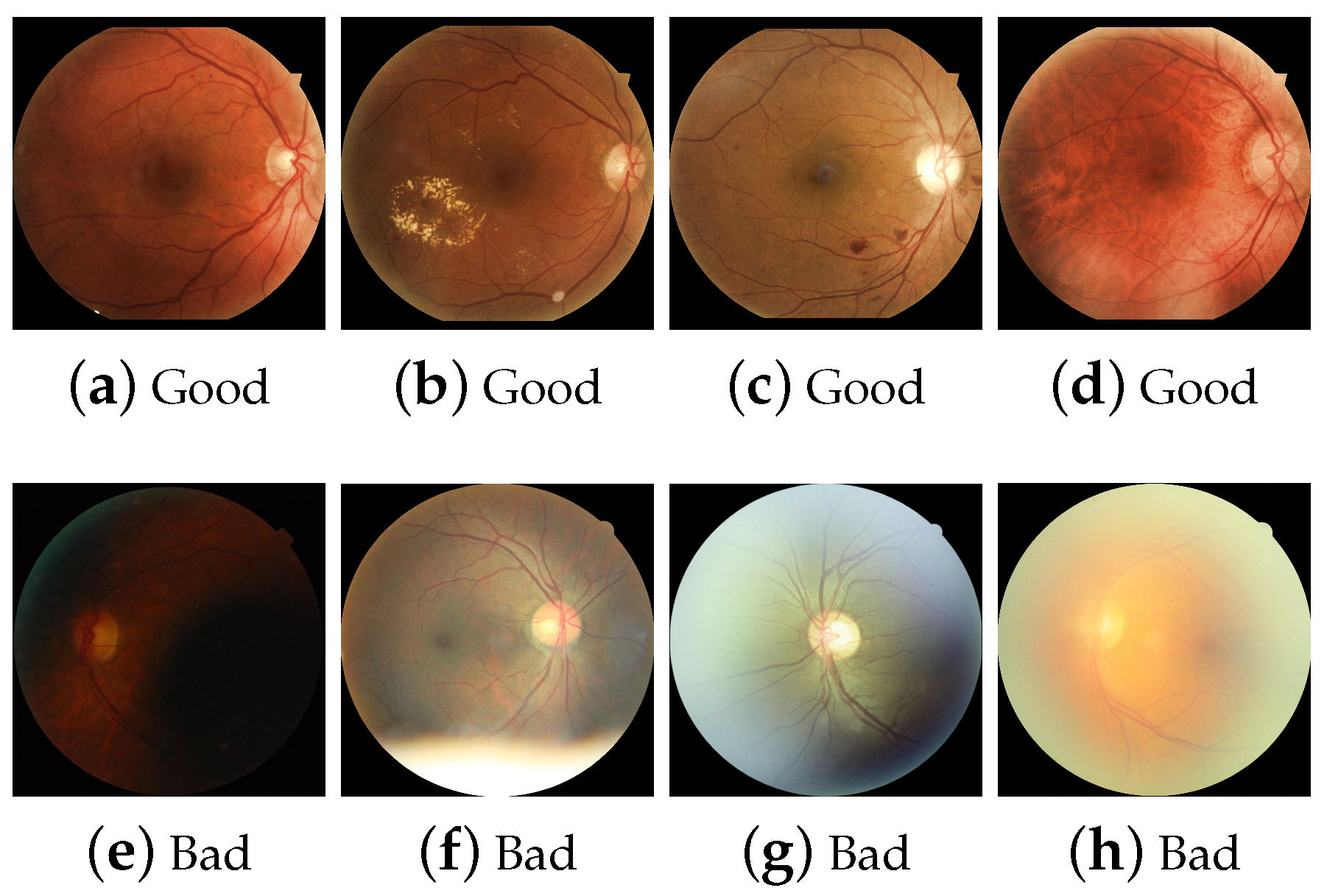
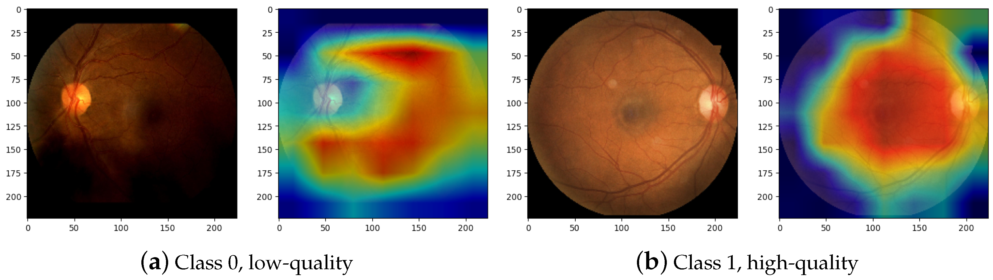
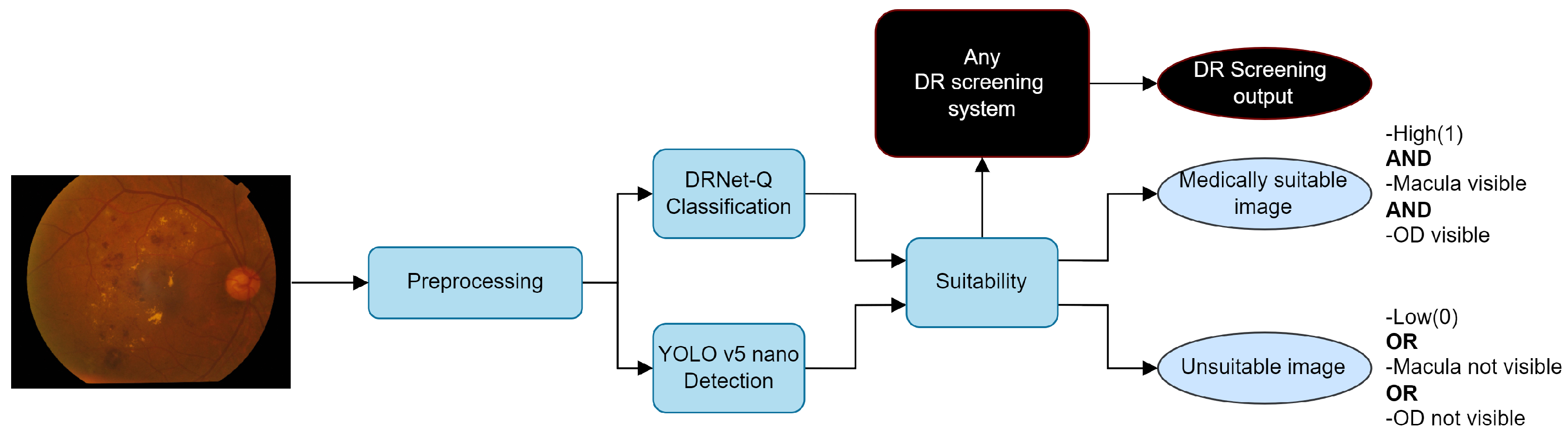
- A lightweight CNN model was proposed for quality binary classification (low and high), which was trained with a dataset generated from public databases in two steps. First, a pre-selection labeling considers quality metrics such as noise, blur, and contrast, as well as the relationship between these metrics. Additionally, an image quality score evaluator assigns a numerical quality level value to each RFI. The second step for labeling is carried out by human judgment based on their visual perception of anatomical features, artifacts, sharpness, and overall visual assessment. Human labeling cannot be solely relied upon due to the possibility of distortions not visible to the human eye. For this, quality metrics, numerical evaluation, pre-selection labeling, and human criteria selection ensure that images correspond to each class.
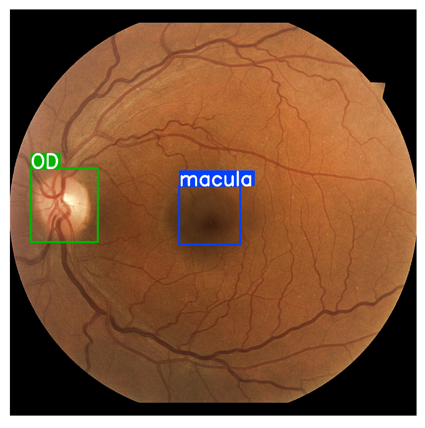
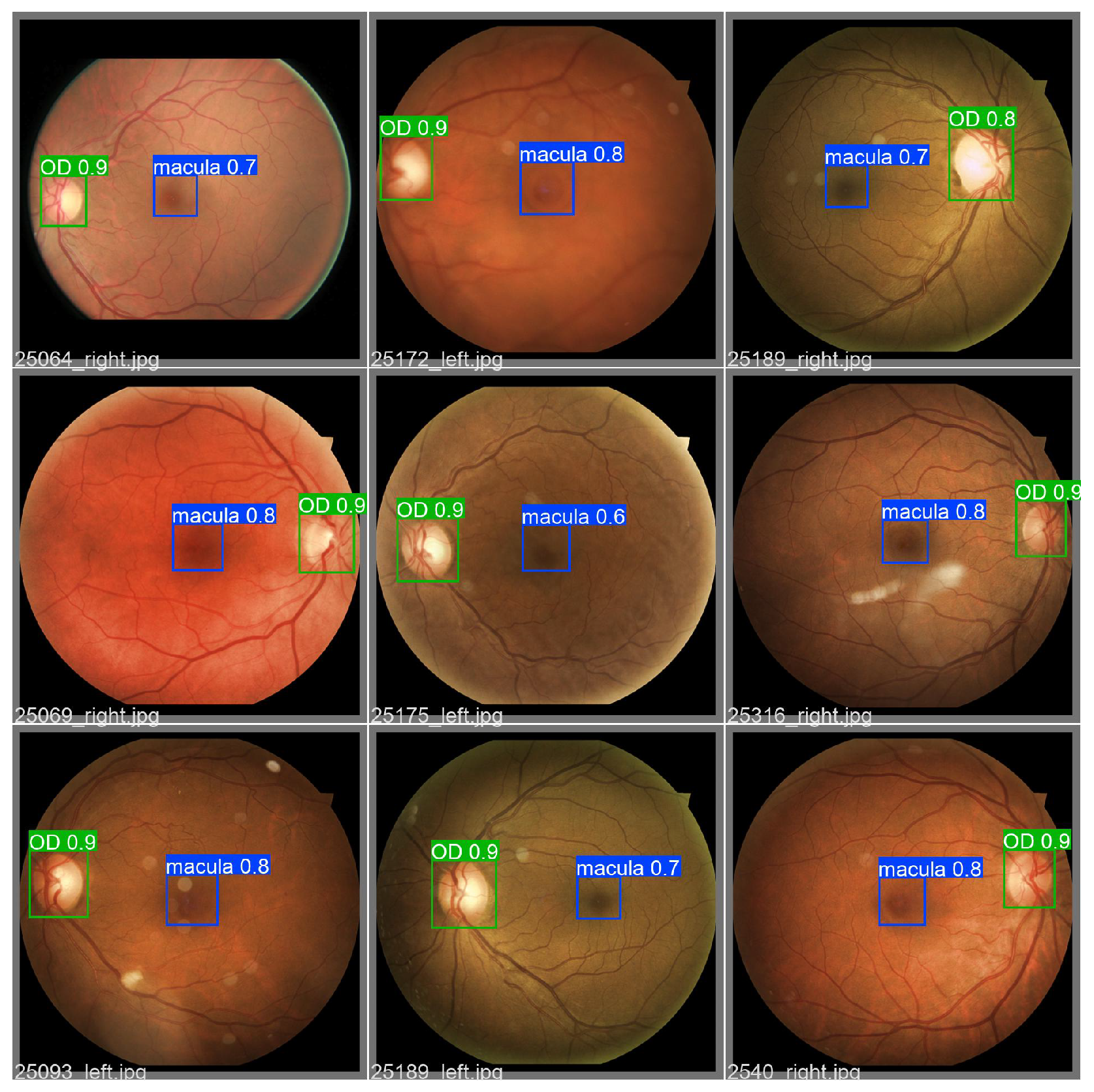
- A small CNN model (YOLOv5 nano) is trained to detect the most relevant regions for DR screening, such as the macula and the OD, in order to ensure the presence of anatomical regions. These two models ensure that making the suitable decision is more transparent because the anatomical features are present.
2. Methods and Data
2.1. Images Dataset
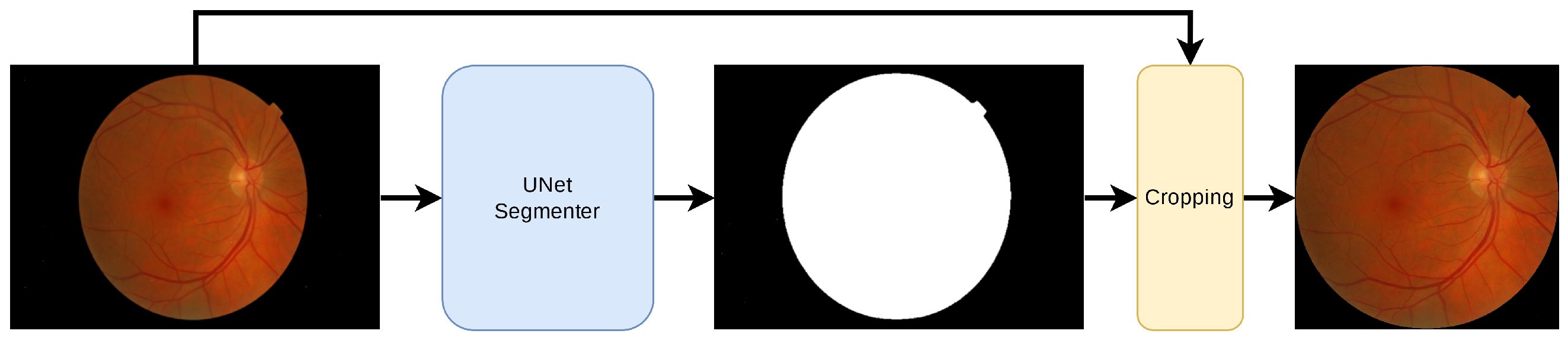
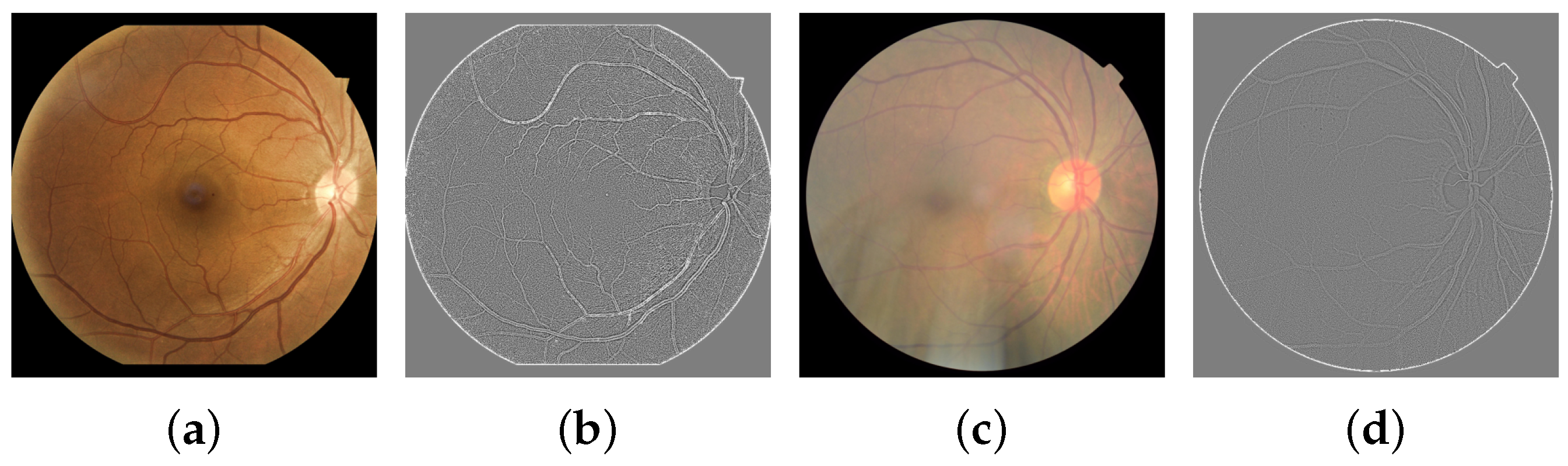
2.2. Pre-Processing
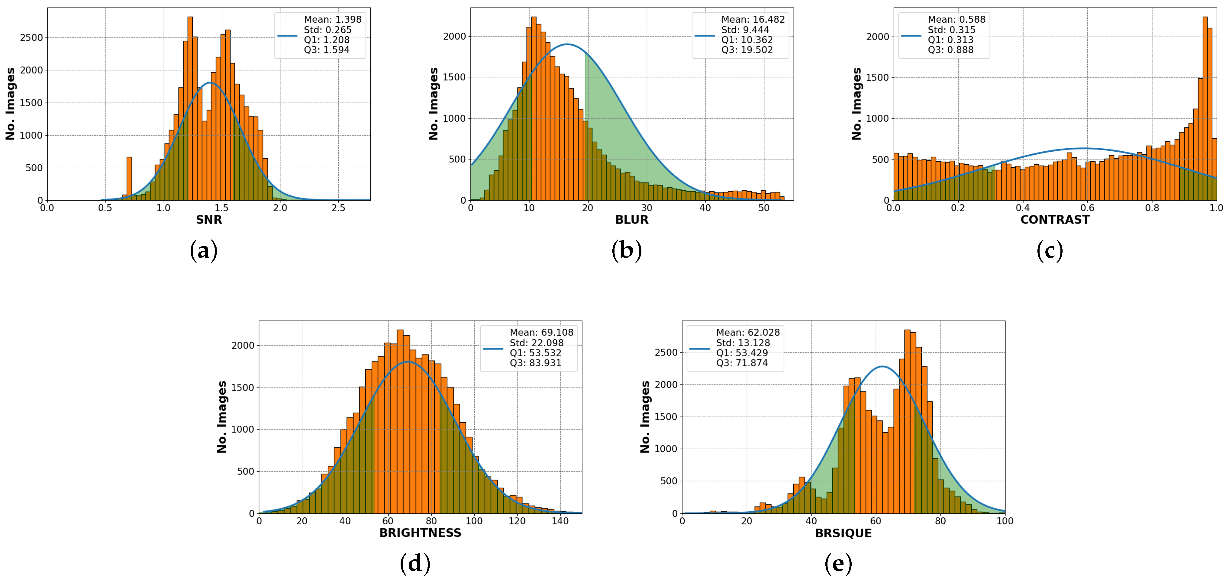
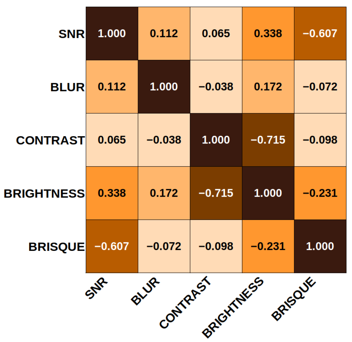
2.3. Image Quality Standard Features
2.4. Image Quality Scoring Evaluator
2.5. Clustering
2.6. Human Visual Opinion
2.7. Classification
2.7.1. CNN-Based Models
2.7.2. Self-Attention Transformers
2.8. Object Detection
3. Results
3.1. Hardware and Resources
3.2. Pre-Processing
3.3. Standard Features and Quality Evaluator
3.4. KMeans
3.5. Classification
3.6. Object Detection
3.7. Suitable RFI for DR
4. Discussion
5. Conclusions
Author Contributions
Funding
Informed Consent Statement
Data Availability Statement
Acknowledgments
Conflicts of Interest
References
- Teo, Z.L.; Tham, Y.C.; Yu, M.; Chee, M.L.; Rim, T.H.; Cheung, N.; Bikbov, M.M.; Wang, Y.X.; Tang, Y.; Lu, Y.; et al. Global Prevalence of Diabetic Retinopathy and Projection of Burden through 2045: Systematic Review and Meta-analysis. Ophthalmology 2021, 128, 1580–1591. [Google Scholar] [CrossRef] [PubMed]
- Guidelines for Diabetic Eye Care; International Council Ophthalmology: Brussels, Belgium, 2017.
- Cole, E.D.; Novais, E.A.; Louzada, R.N.; Waheed, N.K. Contemporary retinal imaging techniques in diabetic retinopathy: A review. Clin. Exp. Ophthalmol. 2016, 44, 289–299. [Google Scholar] [CrossRef] [PubMed]
- Luo, L.; Xue, D.; Feng, X. Automatic Diabetic Retinopathy Grading via Self-Knowledge Distillation. Electronics 2020, 9, 1337. [Google Scholar] [CrossRef]
- Paradisa, R.H.; Bustamam, A.; Mangunwardoyo, W.; Victor, A.A.; Yudantha, A.R.; Anki, P. Deep feature vectors concatenation for eye disease detection using fundus image. Electronics 2022, 11, 23. [Google Scholar] [CrossRef]
- Fan, R.; Liu, Y.; Zhang, R. Multi-Scale Feature Fusion with Adaptive Weighting for Diabetic Retinopathy Severity Classification. Electronics 2021, 10, 1369. [Google Scholar] [CrossRef]
- Pham, Q.T.; Ahn, S.; Song, S.J.; Shin, J. Automatic drusen segmentation for age-related macular degeneration in fundus images using deep learning. Electronics 2020, 9, 1617. [Google Scholar] [CrossRef]
- Ruamviboonsuk, P.; Tiwari, R.; Sayres, R.; Nganthavee, V.; Hemarat, K.; Kongprayoon, A.; Raman, R.; Levinstein, B.; Liu, Y.; Schaekermann, M.; et al. Real-time diabetic retinopathy screening by deep learning in a multisite national screening programme: A prospective interventional cohort study. Lancet Digit. Health 2022, 4, e235–e244. [Google Scholar] [CrossRef]
- Ting, D.S.W.; Cheung, C.Y.L.; Lim, G.; Tan, G.S.W.; Quang, N.D.; Gan, A.; Hamzah, H.; Garcia-Franco, R.; San Yeo, I.Y.; Lee, S.Y.; et al. Development and Validation of a Deep Learning System for Diabetic Retinopathy and Related Eye Diseases Using Retinal Images From Multiethnic Populations With Diabetes. J. Am. Med. Assoc. 2017, 318, 2211–2223. [Google Scholar] [CrossRef] [PubMed]
- Beede, E.; Baylor, E.; Hersch, F.; Iurchenko, A.; Wilcox, L.; Ruamviboonsuk, P.; Vardoulakis, L.M. A Human-Centered Evaluation of a Deep Learning System Deployed in Clinics for the Detection of Diabetic Retinopathy. In Proceedings of the 2020 CHI Conference on Human Factors in Computing Systems, Honolulu, HI, USA, 25–30 April 2020; pp. 1–12. [Google Scholar]
- Gonzalez-Briceno, G.; Sanchez, A.; Ortega-Cisneros, S.; Garcia Contreras, M.S.; Pinedo Diaz, G.A.; Moya-Sanchez, E.U. Artificial Intelligence-Based Referral System for Patients With Diabetic Retinopathy. Computer 2020, 53, 77–87. [Google Scholar] [CrossRef]
- Dodge, S.; Karam, L. Understanding how image quality affects deep neural networks. In Proceedings of the 2016 8th International Conference on Quality of Multimedia Experience (QoMEX), Lisbon, Portugal, 6–8 June 2016; pp. 1–6. [Google Scholar] [CrossRef]
- Zhai, G.; Min, X. Perceptual image quality assessment: A survey. Sci. China Inf. Sci. 2020, 63, 1–52. [Google Scholar] [CrossRef]
- Kamble, V.; Bhurchandi, K.M. Optik No-reference image quality assessment algorithms: A survey. Optik 2015, 126, 1090–1097. [Google Scholar] [CrossRef]
- Niu, Y.; Zhong, Y.; Guo, W.; Shi, Y.; Chen, P. 2D and 3D Image Quality Assessment: A Survey of Metrics and Challenges. IEEE Access 2019, 7, 782–801. [Google Scholar] [CrossRef]
- Stępień, I.; Oszust, M. A Brief Survey on No-Reference Image Quality Assessment Methods for Magnetic Resonance Images. J. Imaging 2022, 8, 160. [Google Scholar] [CrossRef]
- Xu, Z.; Zou, B.; Liu, Q. A Deep Retinal Image Quality Assessment Network with Salient Structure Priors. arXiv 2020, arXiv:2012.15575. [Google Scholar]
- Pires Dias, J.M.; Oliveira, C.M.; da Silva Cruz, L.A. Retinal image quality assessment using generic image quality indicators. Inf. Fusion 2014, 19, 73–90. [Google Scholar] [CrossRef]
- Yao, Z.; Zhang, Z.; Xu, L.Q.; Fan, Q.; Xu, L. Generic features for fundus image quality evaluation. In Proceedings of the 2016 IEEE 18th International Conference on e-Health Networking, Applications and Services (Healthcom), Munich, Germany, 14–17 September 2016; pp. 1–6. [Google Scholar] [CrossRef]
- Yu, F.; Sun, J.; Li, A.; Cheng, J.; Wan, C.; Liu, J. Image quality classification for DR screening using deep learning. In Proceedings of the 2017 39th Annual International Conference of the IEEE Engineering in Medicine and Biology Society (EMBC), Jeju Island, Korea, 11–15 July 2017; pp. 664–667. [Google Scholar] [CrossRef]
- Zago, G.T.; Andreão, R.V.; Dorizzi, B.; Teatini Salles, E.O. Retinal image quality assessment using deep learning. Comput. Biol. Med. 2018, 103, 64–70. [Google Scholar] [CrossRef]
- “EyePACS, Diabetic Retinopathy Detection competition” Kaggle. 2015. Available online: https://www.kaggle.com/c/diabetic-retinopathy-detection/ (accessed on 2 May 2022).
- Clinic, E. Diabetic Retinopathy Segmentation and Grading Challenge. 2012. Available online: https://idrid.grand-challenge.org/Data/ (accessed on 2 May 2022).
- Decencière, E.; Zhang, X.; Cazuguel, G.; Lay, B.; Cochener, B.; Trone, C.; Gain, P.; Ordonez, R.; Massin, P.; Erginay, A.; et al. Feedback on a publicly distributed database: The Messidor database. Image Anal. Stereol. 2014, 33, 231–234. [Google Scholar] [CrossRef]
- 4th Asia Pacific Tele-Ophthalmology Society (APTOS) Symposium. Available online: https://www.kaggle.com/competitions/aptos2019-blindness-detection/overview/description (accessed on 2 May 2022).
- Staal, J.; Abramoff, M.; Niemeijer, M.; Viergever, M.; van Ginneken, B. Ridge based vessel segmentation in color images of the retina. IEEE Trans. Med. Imaging 2004, 23, 501–509. [Google Scholar] [CrossRef]
- Sevik, U. DRIMDB (Diabetic Retinopathy Images Database) Database for Quality Testing of Retinal Images. 2014. Available online: https://academictorrents.com/details/99811ba62918f8e73791d21be29dcc372d660305 (accessed on 2 May 2022).
- Briceno, G.G.; Sánchez, A.; Sánchez, E.U.M.; Cisneros, S.O.; Pinedo, G.; Contreras, M.S.G.; Castillo, B.A. Automatic cropping of retinal fundus photographs using convolutional neural networks. Res. Comput. Sci. 2020, 149, 161–167. [Google Scholar]
- Ronneberger, O.; Fischer, P.; Brox, T. U-Net: Convolutional Networks for Biomedical Image Segmentation. In Proceedings of the Medical Image Computing and Computer-Assisted Intervention—MICCAI 2015, Munich, Germany, 5–9 October 2015; Navab, N., Hornegger, J., Wells, W.M., Frangi, A.F., Eds.; Springer: Cham, Switzerland; pp. 234–241. [Google Scholar]
- Cao, H.; Wang, Y.; Chen, J.; Jiang, D.; Zhang, X.; Tian, Q.; Wang, M. Swin-Unet: Unet-like Pure Transformer for Medical Image Segmentation. arXiv 2021, arXiv:2105.05537. [Google Scholar]
- Mittal, A.; Moorthy, A.K.; Bovik, A.C. No-Reference Image Quality Assessment in the Spatial Domain. IEEE Trans. Image Process. 2012, 21, 4695–4708. [Google Scholar] [CrossRef] [PubMed]
- MacQueen, J. Some methods for classification and analysis of multivariate observations. In Proceedings of the 50th Berkeley Symposium on Mathematical Statistics and Probability, Volume 1: Statistics; University of California Press: Berkeley, CA, USA, 1967; pp. 281–297. [Google Scholar]
- Deng, J.; Dong, W.; Socher, R.; Li, L.J.; Li, K.; Fei-Fei, L. ImageNet: A large-scale hierarchical image database. In Proceedings of the 2009 IEEE Conference on Computer Vision and Pattern Recognition, Miami, FL, USA, 20–25 June 2009; pp. 248–255. [Google Scholar] [CrossRef]
- Szegedy, C.; Vanhoucke, V.; Ioffe, S.; Shlens, J.; Wojna, Z. Rethinking the Inception Architecture for Computer Vision. In Proceedings of the 2016 IEEE Conference on Computer Vision and Pattern Recognition (CVPR), Las Vegas, NV, USA, 27–30 June 2016; pp. 2818–2826. [Google Scholar] [CrossRef]
- He, K.; Zhang, X.; Ren, S.; Sun, J. Deep Residual Learning for Image Recognition. In Proceedings of the 2016 IEEE Conference on Computer Vision and Pattern Recognition (CVPR), Las Vegas, NV, USA, 27–30 June 2016; pp. 770–778. [Google Scholar] [CrossRef]
- Simonyan, K.; Zisserman, A. Very Deep Convolutional Networks for Large-Scale Image Recognition. In Proceedings of the 2015 3rd IAPR Asian Conference on Pattern Recognition (ACPR), Kuala Lumpur, Malaysia, 3–6 November 2015; pp. 730–734. [Google Scholar] [CrossRef]
- Vaswani, A.; Shazeer, N.; Parmar, N.; Uszkoreit, J.; Jones, L.; Gomez, A.N.; Kaiser, L.U.; Polosukhin, I. Attention is All you Need. In Proceedings of the Advances in Neural Information Processing Systems; Guyon, I., Luxburg, U.V., Bengio, S., Wallach, H., Fergus, R., Vishwanathan, S., Garnett, R., Eds.; Curran Associates, Inc.: San Jose, CA, USA, 2017; Volume 30. [Google Scholar]
- Dosovitskiy, A.; Beyer, L.; Kolesnikov, A.; Weissenborn, D.; Zhai, X.; Unterthiner, T.; Dehghani, M.; Minderer, M.; Heigold, G.; Gelly, S.; et al. An Image is Worth 16x16 Words: Transformers for Image Recognition at Scale. In Proceedings of the 9th International Conference on Learning Representations, ICLR 2021, Virtual Event, 3–7 May 2021; Available online: https://openreview.net/forum?id=YicbFdNTTy (accessed on 12 May 2022).
- Liu, Z.; Lin, Y.; Cao, Y.; Hu, H.; Wei, Y.; Zhang, Z.; Lin, S.; Guo, B. Swin transformer: Hierarchical vision transformer using shifted windows. In Proceedings of the IEEE/CVF International Conference on Computer Vision, Montreal, QC, Canada, 11–17 October 2021; pp. 10012–10022. [Google Scholar]
- Hassani, A.; Walton, S.; Li, J.; Li, S.; Shi, H. Neighborhood Attention Transformer. arXiv 2022, arXiv:2204.07143. [Google Scholar]
- Jocher, G.; Stoken, A.; Borovec, J.; NanoCode012; ChristopherSTAN; Changyu, L.; Laughing; Tkianai; Hogan, A.; Lorenzomammana; et al. Ultralytics/yolov5: V3.1—Bug Fixes and Performance Improvements. Zenodo. 2020. Available online: https://zenodo.org/record/4154370 (accessed on 3 May 2022).
- Huang, G.; Liu, Z.; Van Der Maaten, L.; Weinberger, K.Q. Densely Connected Convolutional Networks. In Proceedings of the 2017 IEEE Conference on Computer Vision and Pattern Recognition (CVPR), Honolulu, HI, USA, 21–26 July 2017; pp. 2261–2269. [Google Scholar] [CrossRef]
- Paszke, A.; Gross, S.; Massa, F.; Lerer, A.; Bradbury, J.; Chanan, G.; Killeen, T.; Lin, Z.; Gimelshein, N.; Antiga, L.; et al. PyTorch: An Imperative Style, High-Performance Deep Learning Library. In Advances in Neural Information Processing Systems 32; Wallach, H., Larochelle, H., Beygelzimer, A., d’Alché-Buc, F., Fox, E., Garnett, R., Eds.; Curran Associates, Inc.: San Jose, CA, USA, 2019; pp. 8024–8035. [Google Scholar]
- Yakubovskiy, P. Segmentation Models Pytorch. 2020. Available online: https://github.com/qubvel/segmentation_models.pytorch (accessed on 5 May 2022).
- Selvaraju, R.R.; Cogswell, M.; Das, A.; Vedantam, R.; Parikh, D.; Batra, D. Grad-CAM: Visual Explanations from Deep Networks via Gradient-Based Localization. In Proceedings of the 2017 IEEE International Conference on Computer Vision (ICCV), Venice, Italy, 22–29 October 2017; pp. 618–626. [Google Scholar] [CrossRef]
- Dai, L.; Wu, L.; Li, H.; Cai, C.; Wu, Q.; Kong, H.; Liu, R.; Wang, X.; Hou, X.; Liu, Y.; et al. A deep learning system for detecting diabetic retinopathy across the disease spectrum. Nat. Commun. 2021, 12, 3242. [Google Scholar] [CrossRef]


| Criteria | Description | Decision |
|---|---|---|
| Artifacts | Elements inherent to the camera or the patient or person capturing the image, for example, blur (motion or lens) or light rays entering from an external source... | Presence Absence |
| Sharpness | Distinction of small, medium, and large separable elements. Small may be visible microaneurysms, neovessels, and capillaries, if applicable. Medium may be hemorrhages or exudates. Large may be venous dilation, macula, or OD. | Sharp Not Sharp |
| Field definition | Existence of the RE and the macula and their correct positioning | Correct Incorrect |
| Serious injuries | Injuries severe enough to change the anatomical shape of the retina, such as retinal detachment or large hemorrhages. If present, they are outliers in the quality assessment. | Presence Absence |
| General evaluation | An observer considers the image to be generally gradable. | Gradable Ungradable |
| Layer | Output Shape | Kernel | Padding | Activation | Parameters |
|---|---|---|---|---|---|
| Conv2d_1 | [B, 32, 224, 224] | 5 × 5 | 2 × 2 | ReLU | 2432 |
| BatchNorm | [B, 32, 224, 224] | - | - | - | 64 |
| MaxPooling | [B, 32, 112, 112] | 2 × 2 | - | - | 0 |
| Conv2d_2 | [B, 64, 112, 112] | 5 × 5 | 2 × 2 | ReLU | 51,264 |
| Conv2d_3 | [B, 64, 112, 112] | 5 × 5 | 2 × 2 | ReLU | 102,464 |
| BatchNorm | [B, 64, 112, 112] | - | - | - | 128 |
| MaxPooling | [B, 64, 56, 56] | 2 × 2 | - | - | 0 |
| Conv2d_4 | [B, 128, 56, 56] | 3 × 3 | 1 × 1 | ReLU | 73,856 |
| Conv2d_5 | [B, 64, 56, 56] | 3 × 3 | 1 × 1 | ReLU | 73,792 |
| BatchNorm | [B, 64, 56, 56] | - | - | - | 128 |
| MaxPooling | [B, 64, 28, 28] | 2 × 2 | - | - | 0 |
| Conv2d_6 | [B, 32, 28, 28] | 3 × 3 | 1 × 1 | ReLU | 18,464 |
| Conv2d_7 | [B, 32, 28, 28] | 3 × 3 | 1 × 1 | ReLU | 9248 |
| BatchNorm | [B, 32, 28, 28] | - | - | - | 64 |
| MaxPooling | [B, 32, 14, 14] | 2 × 2 | - | - | 0 |
| Conv2d_8 | [B, 16, 14, 14] | 3 × 3 | 1 × 1 | ReLU | 4624 |
| BatchNorm | [B, 16, 14, 14] | - | - | - | 32 |
| MaxPooling | [B, 16, 7, 7] | 2 × 2 | - | - | 0 |
| Flatten | [B, 784] | - | - | - | 0 |
| Linear | [B, 512] | - | - | ReLU | 401,920 |
| Linear | [B, 2] | - | - | SoftMax | 1026 |
| Total | 739,506 |
| Model | Weight Initialization | No. Params (Mill) | GPU Inference Time (ms) | ||
|---|---|---|---|---|---|
| UNet [29] | Random | 0.467 | 0.0167 | 0.9967 | 8.55 |
| Swin-UNet [30] | Random | 1.7 | 0.0226 | 0.9929 | 38.01 |
| UNet-Resnet18 [44] | ImageNet | 14.3 | 0.0173 | 0.9944 | 13.82 |
| UNet-Resnet50 [44] | ImageNet | 32.5 | 0.0151 | 0.9951 | 28.38 |
| UNet-VGG16 [44] | ImageNet | 23.7 | 0.0173 | 0.9939 | 22.89 |
| Cluster | SNR | Blur | Contrast | Brightness | BRISQUE |
|---|---|---|---|---|---|
| 0 | 1.458 | 23.86 | 0.785 | 88.21 | 72.43 |
| 1 | 1.321 | 11.36 | 0.337 | 52.07 | 54.97 |
| Dataset | Images | K0 | K1 |
|---|---|---|---|
| EyePACS [22] | 35,126 | 10,422 | 24,704 |
| APTOS19 [25] | 5590 | 1389 | 4201 |
| MESSIDOR [24] | 1200 | 6 | 1194 |
| IDRID [23] | 597 | 5 | 592 |
| DRIMDB [27] | 194 | 69 | 125 |
| DRIVE [26] | 40 | 4 | 36 |
| Total | 42,747 | 11,895 | 30,852 |
| Dataset | Images | H0 | H1 | Train | Validation | Test |
|---|---|---|---|---|---|---|
| EyePACS | 35,126 | 2000 | 2000 | 2800 | 600 | 600 |
| Model | Weight Initialization | Image Size (Pixels) | Params (Mill.) | Sensitivity | Specificity | AUC | GPU Inference Time (ms) | ||
|---|---|---|---|---|---|---|---|---|---|
| VGG13 [36] | ImageNet | 224 | 128.9 | 0.0079 | 0.9992 | 0.982 | 0.9833 | 0.986 | 2.930 |
| InceptionV3 [34] | ImageNet | 299 | 25.3 | 0.0117 | 0.960 | 0.98 | 0.96 | 0.985 | 10.410 |
| ResNet18 [35] | ImageNet | 224 | 11.2 | 0.0141 | 0.9964 | 0.98 | 0.9833 | 0.985 | 4.170 |
| ResNet50 [35] | ImageNet | 224 | 23.5 | 0.0089 | 0.9984 | 0.981 | 0.9832 | 0.987 | 6.114 |
| Swin Tiny [39] | ImageNet | 224 | 27.4 | 0.0048 | 0.9992 | 0.9766 | 0.8966 | 0.978 | 8.927 |
| NAT Mini [40] | ImageNet | 224 | 19.5 | 0.0201 | 0.9971 | 0.98 | 0.98 | 0.985 | 10.799 |
| Swin Custom [39] | Random | 224 | 1 | 0.0206 | 0.9964 | 0.9833 | 0.84 | 0.984 | 7.389 |
| NAT Custom [40] | Random | 224 | 1.2 | 0.0029 | 0.9971 | 0.9833 | 0.74 | 0.972 | 4.270 |
| DRNet-Q | Random | 224 | 0.74 | 0.0036 | 0.9984 | 0.9766 | 0.9833 | 0.986 | 1.102 |
| Dataset | Total Images | Localization | Train | Validation |
|---|---|---|---|---|
| EyePACS [22] | 1200 | Macula: 1200 OD: 1200 | 960 | 240 |
| Model | Params (Mill.) | 0.5:0.95 | 0.5 | GFLOPs | GPU Inference Time (ms) |
|---|---|---|---|---|---|
| YOLOv5n | 1.7 | 0.945 | 0.609 | 4.2 | 6.4 |
| YOLOv5s | 7.2 | 0.955 | 0.603 | 15.8 | 6.8 |
| YOLOv5m | 21.2 | 0.961 | 0.602 | 48 | 7.8 |
| YOLOv5l | 46.5 | 0.967 | 0.606 | 107.8 | 10.1 |
| YOLOv5x | 86.7 | 0.962 | 0.597 | 204 | 14.3 |
| Dataset | Total | Macula | OD | Q0 | Q1 | Suitables |
|---|---|---|---|---|---|---|
| EyePACS [22] | 35,126 | 29,284 | 34,130 | 10,724 | 24,402 | 24,125 |
| APTOS [25] | 5590 | 3887 | 5580 | 1635 | 3955 | 3148 |
| MESSIDOR [24] | 1200 | 1128 | 1196 | 99 | 1101 | 955 |
| IDRID [23] | 597 | 562 | 596 | 39 | 557 | 542 |
| DRIMDB [27] | 194 | 77 | 125 | 81 | 124 | 70 |
| DRIVE [26] | 40 | 33 | 39 | 6 | 34 | 32 |
| KMeans (True) | DRNet-Q (Prediction) | Metrics | |||||
|---|---|---|---|---|---|---|---|
| No. Images | K0 | K1 | Q0 | Q1 | Accuracy | Sensitivity | Specificity |
| 42,747 | 11,895 | 30,852 | 12,574 | 30,172 | 0.9523 | 0.9428 | 0.9559 |
Publisher’s Note: MDPI stays neutral with regard to jurisdictional claims in published maps and institutional affiliations. |
© 2022 by the authors. Licensee MDPI, Basel, Switzerland. This article is an open access article distributed under the terms and conditions of the Creative Commons Attribution (CC BY) license (https://creativecommons.org/licenses/by/4.0/).
Share and Cite
Pinedo-Diaz, G.; Ortega-Cisneros, S.; Moya-Sanchez, E.U.; Rivera, J.; Mejia-Alvarez, P.; Rodriguez-Navarrete, F.J.; Sanchez, A. Suitability Classification of Retinal Fundus Images for Diabetic Retinopathy Using Deep Learning. Electronics 2022, 11, 2564. https://doi.org/10.3390/electronics11162564
Pinedo-Diaz G, Ortega-Cisneros S, Moya-Sanchez EU, Rivera J, Mejia-Alvarez P, Rodriguez-Navarrete FJ, Sanchez A. Suitability Classification of Retinal Fundus Images for Diabetic Retinopathy Using Deep Learning. Electronics. 2022; 11(16):2564. https://doi.org/10.3390/electronics11162564
Chicago/Turabian StylePinedo-Diaz, German, Susana Ortega-Cisneros, Eduardo Ulises Moya-Sanchez, Jorge Rivera, Pedro Mejia-Alvarez, Francisco J. Rodriguez-Navarrete, and Abraham Sanchez. 2022. "Suitability Classification of Retinal Fundus Images for Diabetic Retinopathy Using Deep Learning" Electronics 11, no. 16: 2564. https://doi.org/10.3390/electronics11162564
APA StylePinedo-Diaz, G., Ortega-Cisneros, S., Moya-Sanchez, E. U., Rivera, J., Mejia-Alvarez, P., Rodriguez-Navarrete, F. J., & Sanchez, A. (2022). Suitability Classification of Retinal Fundus Images for Diabetic Retinopathy Using Deep Learning. Electronics, 11(16), 2564. https://doi.org/10.3390/electronics11162564