A Novel Seismocardiogram Mathematical Model for Simplified Adjustment of Adaptive Filter

Abstract

Nonclinical measurements of a seismocardiogram (SCG) can diagnose cardiovascular disease (CVD) at an early stage, when a critical condition has not been reached, and prevents unplanned hospitalization. However, researchers are restricted when it comes to investigating the benefits of SCG signals for moving patients, because the public database does not contain such SCG signals. The analysis of a mathematical model of the seismocardiogram allows the simulation of the heart with cardiovascular disease. Additionally, the developed mathematical model of SCG does not totally replace the real cardio mechanical vibration of the heart. As a result, a seismocardiogram signal of 60 beats per min (bpm) was generated based on the main values of the main artefacts, their duration and acceleration. The resulting signal was processed by finite impulse response (FIR), infinitive impulse response (IRR), and four adaptive filters to obtain optimal signal processing settings. Meanwhile, the optimal filter settings were used to manage the real SCG signals of slowly moving or resting. Therefore, it is possible to validate measured SCG signals and perform advanced scientific research of seismocardiogram. Furthermore, the proposed mathematical model could enable electronic systems to measure the seismocardiogram with more accurate and reliable signal processing, allowing the extraction of more useful artefacts from the SCG signal during any activity.

1. Introduction

The heart is one of the most complex and hardest-working organs in the physiological system of a living organism and determines the quality of human life. Proper cardiac diagnosis allows one to notice heart problems in a timely manner. Various cardiac tests are among the most important, but the number of patients with cardiovascular disease remains high [1,2]. One of the most popular heart work measurements is electrocardiogram measurement, but the measurement of electrocardiogram is a clinical method and is not suitable for monitoring the patient’s daily or active activities due to the need to carry uncomfortable electrodes [3,4]. The need for nonclinical monitoring is growing to detect changes in cardiac work at an early stage, to facilitate treatment in areas where cardiac disease experts are missing [5,6]. Additionally, hospitals want to minimize unplanned visits to clinics or hospitals, when majority visits are minute-time and, as a result, not cost beneficial. For this group, the challenge is how to help them to interpret symptoms correctly and alert an ambulance or use medicaments instead of waiting for symptoms to disappear [7,8]. Therefore, the main objective is to reduce mortality by replacing stationary diagnostic devices with portable devices, which can alert to possible disease.

These portable or wearable electronic systems do not disturb the daily activity of patients, have evaluated data noninvasively and extract various information on heart functionality [9,10]. The seismocardiogram signal represents low-frequency (0–50 Hz) cardio cycle mechanic vibrations corresponding to cardiac events [11,12], and contains mitral valve opening (MO) and closing (MC), isovolumetric contraction, ejection, opening of the aortic valve (AO) and closing (AC), and cardiac filling [13]. The heart monitoring system is complicated due to its nonstationary nature [14] and the presence of noises such as muscle movement noise, respiration vibration noise [8], and environment acoustic noise [6,15] in the seismocardiogram (SCG) signal [16,17]. These signals correspond to the surfaces generated by cardiac activities, which we can measure with the accelerometer micromechanical system (electromechanical control system-MEMS) [18]. In addition, we aim to search for other measurement methods and methods, such as forcecardiography (FCG), which describes a combination of force and accelerometer sensors that can monitor weak mechanical oscillations of the heart’s work [19,20].

This article is one of the articles which deals with a moving patient without simultaneously measuring the ECG. Therefore, the development of seismocardiogram measurement devices requires a good understanding of this signal morphology. Using mathematical models of heart and seismocardiogram signals reduces investigation time and resources. The article [21] describes the mechanical morphology of the seismocardiogram and suggests an analytic seismocardiogram model. This model can be complicated, because it requires good heart physiological mechanics and liquid mechanics. Such heartbeat signals can be simulated using an electric circuit heart model, which researchers call a cardiovascular functional avatar [22]. Furthermore, the numeric seismocardiogram model suggests using the artefacts that share the fiducial points of the seismocardiogram from early published studies [11,23]. As a result, the mathematical signal results in further progression of the investigation. The mathematical representation of the human heart allows more accurate and better-quality analysis of the cause of cardiovascular diseases.

The rest of the article is organized as follows. Section 2 discusses related works and methods, describes the mathematical model of seismocardiogram signal and algorithms, and introduces the use of the SCG model and the processing of a real signal with adaptive filters. Section 3 presents the experimental data and analysis. Section 4 concludes the work of this paper and briefly introduces future works.

2. Materials and Methods

The cardiovascular system is complex and, in order to create a mathematical model describing it, it is also complicated. Thus, systematic analysis methods are useful when attention first focuses on the structure of the system, then on the interrelationship of the individual components, and finally on the internal structure of individual parts. For this reason, regarding the cardiovascular system, it is appropriate to investigate the heart separately from blood vessels. In addition, the seismocardiogram investigation is related to the transfer of vibrations from the heart muscles to the chest. Unlike the most popular clinical heart rate monitoring methods, such as electrocardiogram, ultrasound cardiogram, phonocardiogram, or photoplethysmogram, mechanocardiogram measurement is focused on recording and analyzing mechanical vibrations in the heart muscle with micro-electromechanical system (MEMS) sensors [24]. This list can be supplemented with a force sensor consisting of an accelerometer and a force-sensitive resistor [25,26].

2.1. Related Works

The complexity of the human cardiovascular system involves many control mechanisms, which can mathematically explain the proposed nature of the investigation. The heart modeling process has a few directions, mathematical and physical, which have to be followed before real experiments occur [22,27]. Apart from that, the cardiovascular system is generally hydraulic, but also can be analyzed in the electrical circuit [28]. The concept that one heart work cycle or a heartbeat duration combines systolic and diastolic durations unites the hemodynamic and electrical nature of development of an artificial heart or a mathematical model. Due to both models, the general scopes demonstrate parts of impulses rising and falling [27].

Examining the cardiovascular system, researchers in papers point out the heart as a pump forcing blood flow through the blood vessels. Hence, the heart is emphasized as a hydraulic system, which is defined using fluid mechanics equations, quantities, and coefficients such as: vessel volume, blood flow rate, blood pressure, wall elasticity and strength, cross-section area, vessels length, blood viscosity, and blood density [29,30].

The main advantage of this model is that it is directly related to the patient, whose several required quantities (blood viscosity, blood density, blood pressure, etc.) can be measured by laboratory tests inside a medical institution.

Another part of the heart mathematical models is related to the electrical nature of the heart, when an electrical impulse is generated as the synodic node, and as a result, it forces the heart muscle to move periodically [22,31]. These pulses can be measured using electrodes and an electrocardiogram. For this reason, the heart mathematical model is based on an electrical circuit. The aim of this model is to reproduce and simulate an electrocardiogram.

The third part of the mathematical models is the result of changing the hemodynamical representation of the heart to electrical [32,33]. So, the hydraulic system interconnects mechanical and electrical quantities, coefficients and constants [28]. The element of each mechanical system is described by parameters corresponding to the analogy of their mechanical nature. Then, the blood flow in the blood vessels is changed to the electrical current, the volume is changed to voltage, the resistance to blood flow (R) Equation (1) [27] is changed to electrical resistance, blood flow inertia (L) Equation (2) [27] is changed to electrical induction, and the storage (C) Equation (3) [27] is changed to electrical capacity. Hence, nonelectrical quantities are replaced by electrical ones.

$$R=\frac{8l\mu }{\pi r^4}$$

(1)

$$L=\frac{8l\rho }{\pi r^2}$$

(2)

$$C=\frac{3\pi r^{3}l}{2Eh}$$

(3)

where: l—length of the artery; µ—blood viscosity; r—radius; ρ—blood viscosity; h—thickness; and E—Jung module.

The proposed seismocardiogram model in [21] represents blood flow through large vessels in the upper part of the body. The written mathematical model explains the systolic and diastolic phases and forces [34]. This mathematical model is helpful and suited to explaining heart work from a mechanical perspective.

This article is closely related to the previous article of this research group, and will continue the work of improving the quality of the study of nonclinical SCG signals [35]. Also, the work relates to investigations of using wireless sensors and them effective energy consumption [36,37,38]. Direct comparison of a few different models is difficult, it requires a deep understanding of each model. All models discussed require a good understanding of the cardiovascular system and individual parameters of the patients that the mathematical model performs correctly. Thus, a simpler mathematical model is required, which can support researchers in investigating the seismocardiogram or developing new devices for ensuring quality of life and safety in roads [39,40,41,42].

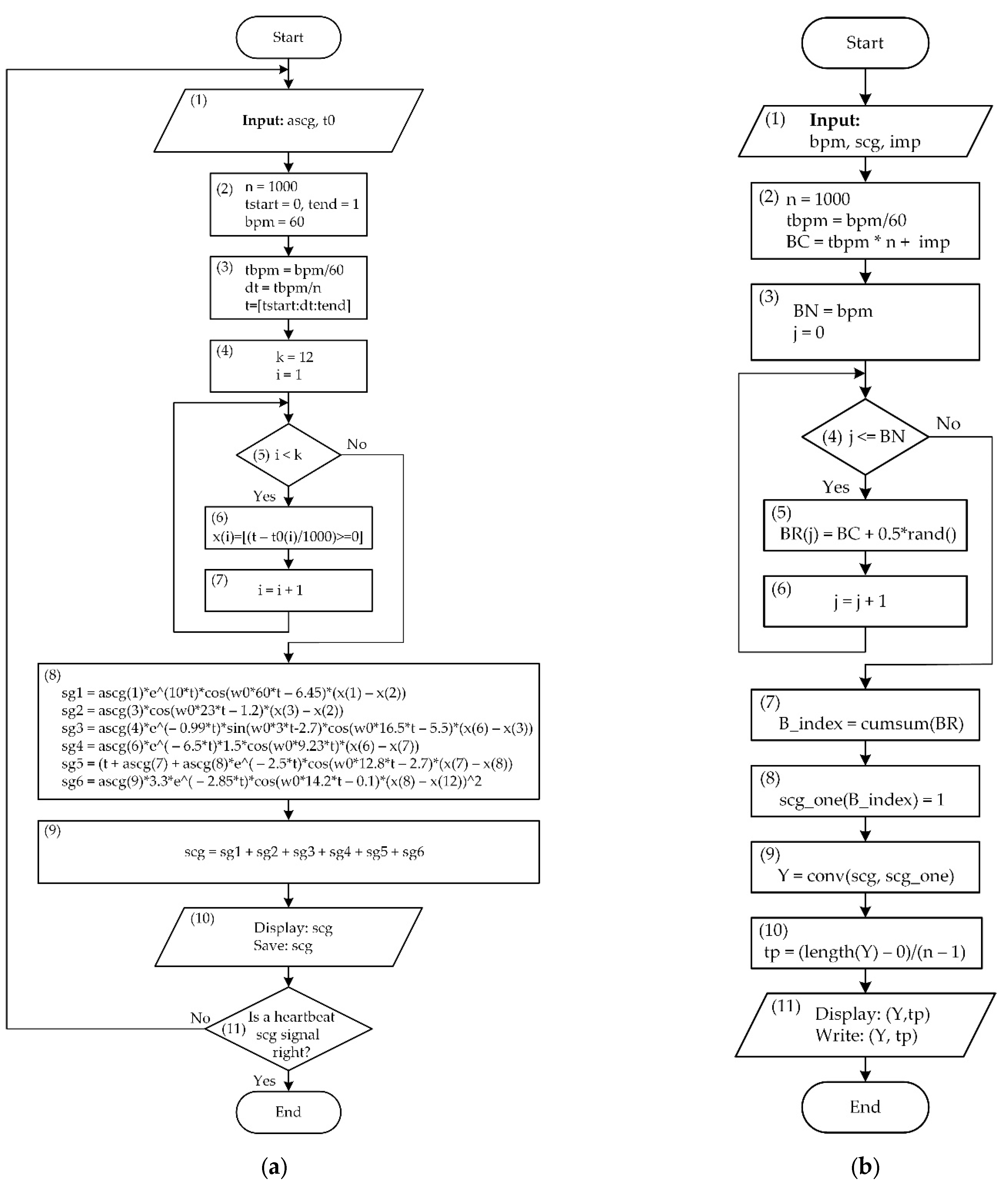
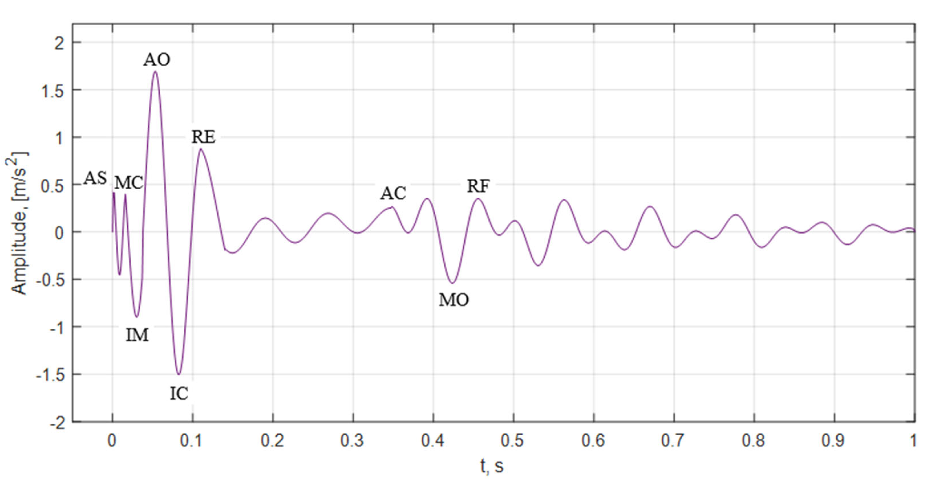
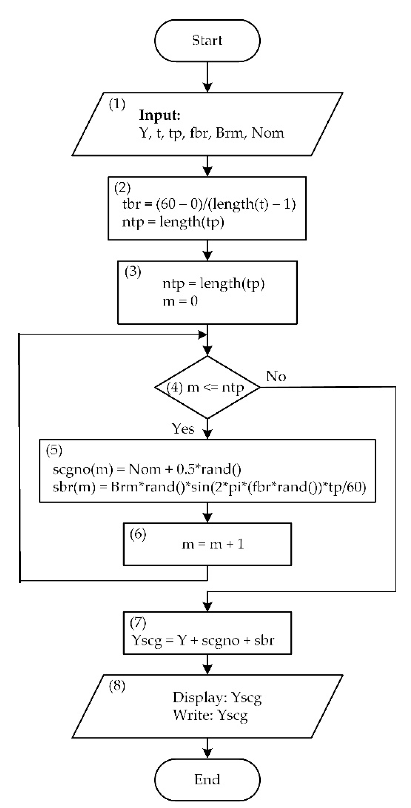
2.2. Mathematical Modeling

A single heartbeat signal mathematical model is created according to the data provided in

Table 1. Seismocardiogram artefacts fiducial points and duration rangers.

Mark	Description	Points from	Points to	Duration, ms
TMC,AO	Duration from MC to AO	16 (±14)	59 (±11)	43 (±14)
TAO,AC	Duration from AO to AC	59 (±11)	348 (±37)	332 (±37)
TMC,MO	Duration from MC to MO	16 (±14)	437 (±37)	378 (±37)
TAC,MO	Duration from AC to MO	348 (±37)	437 (±37)	89 (±37)
TRBE	Duration of Systole		−111 (±24)
TRBF	Duration of Diastole	505 (±41)

. For that purpose, a heartbeat cycle is split into artefacts, symbolizing the duration between the heart valves’ state moments. These durations can be recorded in the aria of fiducial points values (4).

$$F{V}_{SCG}=\left\{T^{MC, AO},T^{A0, AC},T^{A0, AC},T^{AC,MO},T^{RBE},T^{RBF}\right\}$$

(4)

where:

• $F{V}_{SCG}$—seismocardiogram signal fiducial points values aria;
• T^MC,AO—time between the aorta opening and closing;
• T^A0,AC—time between the aorta opening and closing;
• T^MC,MO—time between the closing and opening of the mitral valves;
• T^AC,MO—time between the closure of the aorta and the opening of the mitral valve;
• T^RBE—duration of systole;
• T^RBF—duration of diastole.

This passion in the MATLAB program is converted into a single line matrix with additional variables to mark the relative acceleration of the accelerometer ± ag, where a is the measured multiplier and g is the free acceleration equal to 9.8 [m/s²]. The mathematical model of the theoretical SCG signal has been modeled by taking conditional acceleration values from graphics and fiducial points data from other research publications, such as [11] and [15].

The graphics shown in the second picture reflect the main artefacts of the seismocardiogram signal corresponding to the heart working moments specified in Table 1.

The widely visible artefacts of the time values and duration ranges of the seismocardiogram between two fiducial points are shown in the first table, which was created based on [11,23].

The acceleration amplitude values are tabled in

Table 2. Modeled SCG signal acceleration amplitude values and description.

Mark	Acceleration Amplitude Value, m/s2	Description
ascg1	0.5	Arteries systole
ascg2	0.3	Mitral valve closing
ascg3	−0.9	Isovolumetric moment
ascg4	1.8	Aorta valve opening
ascg5	−1.65	Isovolumic contraction
ascg6	1.2	Rapid systole ejection
ascg7	−0.2	Rapid filling
ascg8	0.25	Aorta valve closing
ascg9	−0.55	Mitral valve opening

and explain all the meanings of the abbreviations in more detail.

The proposed time values for each fiducial points are tabled and more details are described in

Table 3. Modeled SCG signal fiducial points time values and description.

Mark	Fiducial Points Time Values, ms	Description
tas	1	Arteries systole
tmc	16	Mitral valve closing
tim	21.5	Isovolumetric moment
tao	59	Aorta valve opening
tic	26	Isovolumic contraction
trbe	111	Rapid systole ejection
trbee	141	Rapid filling
tac	348	Aorta valve closing
tmo	437	Mitral valve opening

.

The mathematical model of the SCG signal was formed based on the Heaviside function, which marks the concrete fiducial points impulse activation sequence in the time domain.

$$s{g}_1\left(t\right)=asc{g}_1{e}^{-10t}\cos \left(w_{o}60t-6.45\right)\left(x_1-x_2\right)$$

(5)

$$s{g}_2\left(t\right)=asc{g}_{3}cos\left(w_{o}23t-1.2\right)\left(x_3-x_2\right)$$

(6)

$$s{g}_3\left(t\right)=asc{g}_4{e}^{-0.98t}\sin \left(w_{o}3t-2.7\right)\cos \left(w_{o}16.5t-5.5\right)\left(x_6-x_3\right)$$

(7)

$$s{g}_4\left(t\right)=asc{g}_6{e}^{-6.5t}1.5\cos \left(w_{o}9.23t\right)\left(x_6-x_7\right)$$

(8)

$$s{g}_5\left(t\right)=\left(t+asc{g}_7+asc{g}_8{e}^{-2.5t}\cos \left(w_{o}12.8t-2.7\right)\right)\left(x_7-x_8\right)$$

(9)

$$s{g}_6\left(t\right)=asc{g}_{9}3.3e^{-2.85t}\cos \left(w_{o}4.1t+3.14\right)\cos \left(w_{o}14.2t-0.1\right){\left(x_8-x_{12}\right)}^2$$

(10)

where:

$w_o=2\pi f$ angular frequency rad/s when f = 1 Hz; sg₁(t)–sg₆(t)—intermediate signal parts, which represent each acceleration artifact of the modeled SCG signal.

The presented equations are intermediate, and form the final expression of the modeled signal scg(t) Equation (11). Each of these formulas is directly related to the seismocardiogram artifacts described in Table 2 and Table 3. On the basis of these artifact values, the artificial signal is developed. Additionally, the synthesis of this signal is made possible, according to investigation requirements, by changing these values.

Adding all the expressions of the signal pulse sequences, a mathematical model of a single heartbeat seismocardiogram signal is obtained, as is the algorithm described in Figure 1, for which the signal is shown in Figure 2.

Following the algorithm described in Figure 1a, the seismocardiogram of a single heartbeat is visualized graphically, so Figure 2 shows the generated theoretical seismocardiogram signal with the main artefacts of a seismocardiogram. So, using this signal the sequence can be produces (Figure 3).

As a result, the mathematical model has been developed on the basis of these artefacts points. In this article, the general Equation (11) is presented and used for the described investigation.

$$scg\left(t\right)=s{g}_1\left(t\right)+s{g}_2\left(t\right)+s{g}_3\left(t\right)+s{g}_4\left(t\right)+s{g}_5\left(t\right)+s{g}_6\left(t\right)$$

(11)

More detail and a clear explanation of the numerically modeled seismocardiogram signal, sequence creation, and management possibilities with additional noises is described using three algorithms (Figure 1 and Figure 4).

The algorithm shown in Figure 1a explains the mathematical model of the seismocardiogram. The main aim of this algorithm is to generate a single-heartbeat SCG signal with one-second duration, then the heart rate is 60 bpm. In the first step of the algorithm, two sets of acceleration values ascg and the corresponding fiducial points time values t0 are entered. These values are the main artifacts of the simulated SCG signal, and sample values for these sets, respectively, are given in Table 2 and Table 3. The researcher can modify these values according to the investigation objectives.

The second step specifies the time constant of the start and end of the heartbeat signal (tstart), the heart rate of 60 bpm and the number of samples number n = 1000. In the third step, the calculations of the required pulse durations are performed and the duration of the sampling step dt creates a 1000 ms time domain.

The 4th, 5th, 6th, and 7th steps of the algorithm show how to find the unit impulse values (x1: x12) corresponding to the time references of the t0 set for creation of a desired shape in the 8th and 9th step of the seismocardiogram signal. The SCG signal is displayed graphically, and all values are stored in the memory during the 10th step of the algorithm. The researcher qualifies a visually received SCG signal in the 11th step and, if required, changes the values of ascg and t0 sets. The researcher can modify the t0 set time values of each fiducial point and parallelly acg set the amplitude values that allow synthesis of the desired SCG signal and allow random changes to be set.

The second algorithm, shown in Figure 1b, describes the simulation of a sequence of SCG signals. This sequence is an analogy of a repetitive heart rhythm. In the first step of the algorithm, the scg signal of one heartbeat obtained in the first algorithm is used. In addition, the heart rate bpm and the number of additional pulses are examined, so that the signals of individual beats do not overlap in the sequence. The next step of the algorithm is to calculate the beat count BC of the sequence. In the following 4th, 5th, and 6th steps, a different number of pulses are counted in the sequence of the SCG signal for each heartbeat. In the seventh step, each heartbeat is given an index and is equated to a unit in Step 8. In Step 9, the sequence Y of the SCG signals is found after the convulsion between the single heartbeat signal scg and the new unit pulse sequences scg_one (B_index) formed in the 9th step, the time counts of which are calculated in the 10th step. In the 10th step of the algorithm, the sequence of the noise-free SCG signal shown in Figure 3 is represented graphically.

From one generated theoretical seismocardiogram cycle, we can create a sequence of desired duration SCG signal without noise, which is shown in Figure 3.

The sequence of SCG signals without noise is not informative and needs to be added with some real noise, which makes the artificial SCG signal more realistic. So, the desired sequence has been constructed with different types of noises, which changes randomly and reflects the real situation. Figure 4 shows the next step, which describes the SCG signal required to perform the sequence with added noise. Thus, the real situation is reflected as a seismocardiogram is measured from a patient and has noncardiac signals that are considered noise. These may be random vibrations in the surrounding environment or chest vibrations caused by breathing.

The algorithm shown in Figure 4 describes the acquisition of an SCG signal with total noise and will be further used to find the optimal parameters of the adaptive filter. First, the parameter values require the Y and t of SCG signal sequences to be entered without the noise, in addition to the respiration rate fbr and its amplitude Brm, and the white noise amplitude Nom. The following four, five, and six steps of the algorithm describe the finding of random values for white noise and respiration. Additionally, the respiration amplitude and frequency vary randomly. In the seventh step, an SCG signal with noise Yscg is obtained, displayed graphically (Figure 5), and saved. Figure 5 shows an example of such a signal. The mathematical model created first allows us to model the desired seismocardiogram signals, monitoring the reaction of the designed system to them, adding various environmental noise signals, and taking into account the research objectives. On the basis of the obtained results, it is possible to develop and research real seismocardiogram measuring devices, which are capable of processing nonclinical data much more efficiently. The legal regulations related to testing medical devices before they are approved and approved are avoided. Additionally, research becomes safer and more economical in this way because optimal data obtained from many simulations are used to realize a real electronic device.

Therefore, an example is presented that examines how the settings of an adaptive filter operating with the least mean squares (LMS) algorithm are obtained after performing signal processing simulations. On the basis of these results, a real electronic measuring device is established, which measures the heart work of one of the authors. Figure 6 shows the method how accelerometer is placed.

Adaptive filtering has many advantages and is useful for biomedical applications when the filter coefficients self-adjust to a rapidly and unpredictably changing signal. The principle of operation of the adaptive filter is defined by Equation (12) [43,44].

$$e\left(n\right)=d\left(n\right)-y\left(n\right)$$

(12)

where: e(n)—adaptation error, y(n)—denoised signal in output, d(n)—desired signal.

The operation of this filter is based on the tendency of the filter output signal y(n) defined by Equation (13) to correspond as closely as possible to the affected signal d(n) through the feedback response of the error signal e(n) to the coefficients H(z) of the filter transfer function, so that e(n) is zero [43,44].

$$y\left(n\right)={\displaystyle \sum }_{k=1}^L{b}_n\left(n\right)x\left(n-k\right)$$

(13)

The structure shows in Figure 7 that, based on the fact that the SCG signal is measured in the frequency band 1–20 Hz. It feeds the signal of the frequency band of interest to the adaptive filter to make the adaptive filter much more efficient and effective [23,45]. For this, a finite impulse response filter (FIR) or an infinite impulse response filter (IIR) can be used [44,46]. As a result, an accelerometer can be used for measurement. Apart from the fundamental adaptive filter configuration, the frequency band is 5–45 Hz for adaptive filter with delay Figure 7. Additionally, the performance to detect AO peaks is analyzed with FIR and IRR filters.

Processing data from the simulated SCG are presented in the

Table 4. Modeled SCG signal processing data.

Filter Order	1 Adaptive Filter	2 Adaptive Filter
Filter Order	FIR (100)/892	IIR (5)/892
mu AF step	2.3105 × 10−4	1.9370 × 10−4
Heart Rate, beats/min	67	69
RMS, m/s2	0.2145	0.2635
SNR, dB	−6.3288	−6.7995
RMSE, m/s2	0.1447	0.3401
Peaks number	63	67
Peaks Interval Mean, ms	887.032	858.313
Peaks Interval STD	446.838	237.043
Adaptation duration, s	1.237476	1.185759
Adaptation time, s	1.200769	1.193749

. The second table shows the measurement results with an adjusted 410 ms duration window, which indicates the shortest interval between the AO peaks [47]. This duration is taken from the data in Table 1 to avoid misinterpretation of seismocardiogram signal artifacts when aortic valve closure is accepted for aortic opening. A mitral valve opening peak may also be faulty. The minimum peak interval can also be called a blind zone or a silence mode, when signal peaks are not evaluated with a level higher than the lowest signal root mean square (RMS) value [48,49]. For the first adapter filter (AF), the convergence parameter or the adaptation step mu is equal to 0.00023, and for the second, this parameter is 0.00019.

Knowing that the signal noise ratio (SNR) [50,51] of the SCG signal at the adaptive filters input is −14.009 dB, the processing efficiencies of these two filters can be evaluated. The processing benefit of the first adaptive filter 7.6802 dB is achieved in 1.2375 s, while the 7.2095 dB processing benefit of the second adaptive filter is achieved in 1.1857 s. The root mean square error (RMSE) of the modeled seismocardiogram signal for the first adaptive filter is 0.1447 (m/s²), and for the second it is 0.3401 (m/s²). Hence, the modeled seismocardiogram signal processing is less stable using the second adaptive filter.

3. Results and Discussions

Based on the data described above, signal processing is performed in the form of a mathematical model of the SCG signal and adaptive filter algorithms. The signal processing is carried out in an experimental way, measured following the theoretical SCG model during desk work when slow moving or in a resting state.

The severity of the generalized seismocardiogram was primarily analyzed by filters of limited and unlimited impulsive reactions. For this purpose, there were limited pulse and indefinite impulsive reaction filters, based on the available initial data suggesting that it is appropriate to examine the signal from the frequency band 1 to 40 Hz.

Ascertainment of whether the limits of the frequency band in question are correctly selected and whether efficient use of the signal processing system resources is performed by a fast Furrier transformation (FFT).

The FFT is performed for the investigated signal when a frequency distribution spectrum is generated which contains the maximum signal powers located in the adjusted frequency band from 0 to 50 Hz.

Similarly, the processing of further SCG signals and its results are focused on the seismocardiogram measurement in order to determine the working condition of the human heart using a nonelectrical measurement method. This choice is motivated by the fact that it is possible to perform an evaluation of a heart condition without disturbing the activity of the patient. The accelerometer, in response to mechanical movements, captures changes in acceleration and converts them into electrical signals. Heart rate is one of the main objects of measurement and is simply determined to give a minimal indication of the state of health.

In order to achieve more reliable data, FIR and IIR filters are applied, which are serially connected with signal delay before the adaptive filter. The decision to use one of the FIR or IIR filters at the beginning will facilitate the adaptive filter’s ability to effectively eliminate suddenly changed signal components related to movement or activity. This responds directly to the purpose of the study and research group to measure the seismocardiogram while the patient performs daily activities such as driving. Based on this, the heart rhythms of the possible scenarios are calculated simultaneously with the evaluation of the time of SCG signal processing using adaptive filter. All seismocardiogram signal processing was performed with MATLAB 2021a software installed on an Intel (R) Core (TM) i5-7200U CPU @2.50 GHz 2.70 GHz with 16 GB of RAM and 109 GB of free space on a 500 GB SSD.

The analyzed resting SCG signal consists of 61,000 samples, which were recorded at a sampling rate of 490 Hz on an MPU9250 accelerometer connected to an ESP32 WROOM microcontroller via an I2C data bus. The measured data analysis was performed with MATLAB software.

After representative calculation of the signals of all three coordinate axes of the accelerometer was performed, a steady-state SCG signal with an SNR of −12.5946 dB was measured.

Figure 8 and Figure 9 shows signal processing results, where (a) signal represents the measured signal in the input.

Figure 8 and Figure 9 show two cases of the measured SCG signal processing data when two different LMS adaptive filter algorithms were adjusted based on the mathematical model simulation data. Both Figure 8 and Figure 9 allow received values of the acceleration amplitudes and fiducial points, which make it possible to perform a deeper analysis of received data, calculate heart rate and heart rate variability.

Following the theoretical seismocardiogram processing data, the same adjustments use adaptive filters for real seismocardiogram signal processing. These processing data are tabled in

Table 5. Rest SCG signal processing data.

Filter Order	1 Adaptive Filter	2 Adaptive Filter
Filter Order	FIR (100)/892	IIR (5)/892
mu AF step	3.5503 × 10−4	5.1336 × 10−4
Heart Rate, beats/min	107	98
RMS, m/s2	0.5503	0.0523
SNR, dB	−5.1047	−7.8809
RMSE, m/s2	0.0717	0.0945
Peaks number	106	97
Peaks Interval Mean, ms	556.406	611.619
Peaks Interval STD	137.600	171.220
Peaks Variation	18,933.805	29,316.363
Adaptation time, s	1.200769	1.193749

.

The 7.49 dB processing benefit of the first adaptive filter was achieved in 1.2 s, while the 4.7137 dB processing benefit of the second adaptive filter was achieved in 1.194 s.

Correlation analysis of the two signals showed that for the filter with a 5 s delay and an IIR filter at the input, the processed steady-state SCG signal level is sufficient and, in some cases, correlates with the SCG-modeled signal without noise signal. Therefore, the adaptive filters must be combined individually (

Table 6. Rest SCG signal processing data with individually adjusted adaptive filters.

Filter Order	3 Adaptive Filter	4 Adaptive Filter
Filter Order	200	50
mu AF step	2.1226 × 10−3	1.4774 × 10−1
Heart Rate, beats/min	95	88
RMS, m/s2	0.4373	0.0478
SNR, dB	−9.0627	−14.9807
RMSE, m/s2	0.0503	0.0984
Peaks number	61	57
Peaks Interval Mean, ms	623.885	664.281
Peaks Interval STD	229.843	132.981
Peaks Variation	52,827.737	17,683.920
Processing time, s	1.091161	1.110726

) to achieve the desired processing results. The negative SNR value in both cases −5.1 and −7.88 dB indicate that denoised signal has a significant level of noise.

Both adaptive filters have been adjusted by reducing filter orders, respectively, from 892 to 200 and 50. Figure 10 represents the seismocardiogram signal in the second adaptive filter with marked AO and AC artifacts.

Figure 11 presents the same signal power frequency density, where one can see the extremums of signal amplitude and artifacts sequences. White spaces indicates each HR cycle signal peaks maximum power in dB.

4. Conclusions

A simpler mathematical model was developed and three algorithms were created for a more detailed explanation and understanding of the process and behavior of the model. Using this algorithm, the processing program can be written in several programming languages, not only in MATLAB. This seismocardiogram model can be used to find optimal parameters (fifth-order delay before adaptive filter, 892 filter order) for adaptive filters that can perform real cardio-mechanical vibration signal processing for estimating AO peaks. As a result, the heart rate was calculated. However, filter order 200 and 50 were evaluated again, so the processing duration decreased in both filters, respectively, from 1.20 to 1.09 and from 1.19 to 1.11 s. In each case, the signal processing and the necessary calculations were performed with programs written in MATLAB.

The proposed system and methodology can be useful to increase such research efficiency. Furthermore, future works will relate to improvements in processing methods by including machine learning to estimate systolic and diastolic intervals and heart rate variability during daily activity.

References

1. Virani, S.S.; Alonso, A.; Aparicio, H.J.; Benjamin, E.J.; Bittencourt, M.S.; Callaway, C.W.; Carson, A.P.; Chamberlain, A.M.; Cheng, S.; Delling, F.N.; et al. Heart Disease and Stroke Statistics—2021 Update. Circulation 2021, 143, E254–E743. [Google Scholar] [CrossRef] [PubMed]
2. Bhatnagar, P.; Wickramasinghe, K.; Wilkins, E.; Townsend, N. Trends in the epidemiology of cardiovascular disease in the UK. Heart 2016, 102, 1945–1952. [Google Scholar] [CrossRef] [PubMed]
3. Saini, S.K.; Gupta, R. Artificial intelligence methods for analysis of electrocardiogram signals for cardiac abnormalities: State-of-the-art and future challenges. Artif. Intell. Rev. 2022, 55, 1519–1565. [Google Scholar] [CrossRef]
4. Maršánová, L.; Ronzhina, M.; Smíšek, R.; Vítek, M.; Němcová, A.; Smital, L.; Nováková, M. ECG features and methods for automatic classification of ventricular premature and ischemic heartbeats: A comprehensive experimental study. Sci. Rep. 2017, 7, 11239. [Google Scholar] [CrossRef] [Green Version]
5. Miramontes, R.; Aquino, R.; Flores, A.; Rodríguez, G.; Anguiano, R.; Ríos, A.; Edwards, A. PlaIMoS: A Remote Mobile Healthcare Platform to Monitor Cardiovascular and Respiratory Variables. Sensors 2017, 17, 176. [Google Scholar] [CrossRef] [PubMed] [Green Version]
6. D’Mello; Skoric; Xu; Roche; Lortie; Gagnon; Plant Real-Time Cardiac Beat Detection and Heart Rate Monitoring from Combined Seismocardiography and Gyrocardiography. Sensors 2019, 19, 3472. [CrossRef] [PubMed] [Green Version]
7. Mehrang, S.; Jafari Tadi, M.; Lahdenoja, O.; Kaisti, M.; Vasankari, T.; Kiviniemi, T.; Airaksinen, J.; Pankaala, M.; Koivisto, T. Machine Learning Based Classification of Myocardial Infarction Conditions Using Smartphone-Derived Seismo- and Gyrocardiography. In Proceedings of the Computing in Cardiology; IEEE Computer Society, Maastricht, The Netherlands, 23–26 September 2018; Volume 45. [Google Scholar]
8. Andreozzi, E.; Centracchio, J.; Punzo, V.; Esposito, D.; Polley, C.; Gargiulo, G.D.; Bifulco, P. Respiration Monitoring via Forcecardiography Sensors. Sensors 2021, 21, 3996. [Google Scholar] [CrossRef]
9. Di Rienzo, M.; Vaini, E.; Castiglioni, P.; Merati, G.; Meriggi, P.; Parati, G.; Faini, A.; Rizzo, F. Wearable seismocardiography: Towards a beat-by-beat assessment of cardiac mechanics in ambulant subjects. Auton. Neurosci. Basic Clin. 2013, 178, 50–59. [Google Scholar] [CrossRef]
10. Polley, C.; Jayarathna, T.; Gunawardana, U.; Naik, G.; Hamilton, T.; Andreozzi, E.; Bifulco, P.; Esposito, D.; Centracchio, J.; Gargiulo, G. Wearable Bluetooth Triage Healthcare Monitoring System. Sensors 2021, 21, 7586. [Google Scholar] [CrossRef]
11. Sahoo, P.K.; Thakkar, H.K.; Lin, W.Y.; Chang, P.C.; Lee, M.Y. On the design of an efficient cardiac health monitoring system through combined analysis of ECG and SCG signals. Sensors 2018, 18, 379. [Google Scholar] [CrossRef] [Green Version]
12. Nguyen, T.-N.; Nguyen, T.-H. Deep Learning Framework with ECG Feature-Based Kernels for Heart Disease Classification. Elektron. Elektrotechnika 2021, 27, 48–59. [Google Scholar] [CrossRef]
13. Taebi, A.; Solar, B.; Bomar, A.; Sandler, R.; Mansy, H. Recent Advances in Seismocardiography. Vibration 2019, 2, 64–86. [Google Scholar] [CrossRef] [PubMed] [Green Version]
14. Jain, P.K.; Tiwari, A.K. Heart monitoring systems-A review. Comput. Biol. Med. 2014, 54, 1–13. [Google Scholar] [CrossRef]
15. Aboltins, A.; Pikulins, D.; Grizans, J.; Tjukovs, S. Piscivorous Bird Deterrent Device Based on a Direct Digital Synthesis of Acoustic Signals. Elektron. Elektrotechnika 2021, 27, 42–48. [Google Scholar] [CrossRef]
16. Conn, N.J.; Schwarz, K.Q.; Borkholder, D.A. In-home cardiovascular monitoring system for heart failure: Comparative study. JMIR mHealth uHealth 2019, 7, e12419. [Google Scholar] [CrossRef]
17. Sahoo, P.K.; Thakkar, H.K.; Lee, M.Y. A cardiac early warning system with multi channel SCG and ECG monitoring for mobile health. Sensors 2017, 17, 711. [Google Scholar] [CrossRef] [PubMed]
18. Leitão, F.; Moreira, E.; Alves, F.; Lourenço, M.; Azevedo, O.; Gaspar, J.; Rocha, L.A. High-Resolution Seismocardiogram Acquisition and Analysis System. Sensors 2018, 18, 3441. [Google Scholar] [CrossRef] [Green Version]
19. Andreozzi, E.; Fratini, A.; Esposito, D.; Naik, G.; Polley, C.; Gargiulo, G.D.; Bifulco, P. Forcecardiography: A Novel Technique to Measure Heart Mechanical Vibrations onto the Chest Wall. Sensors 2020, 20, 3885. [Google Scholar] [CrossRef]
20. Andreozzi, E.; Gargiulo, G.D.; Esposito, D.; Bifulco, P. A Novel Broadband Forcecardiography Sensor for Simultaneous Monitoring of Respiration, Infrasonic Cardiac Vibrations and Heart Sounds. Front. Physiol. 2021, 12, 725716. [Google Scholar] [CrossRef]
21. Holcik, J.; Moudr, J. Mathematical Model of Seismocardiogram. In World Congress on Medical Physics and Biomedical Engineering 2006; Springer: Berlin/Heidelberg, Germany, 2007; Volume 14, pp. 3415–3418. [Google Scholar]
22. Casas, B.; Lantz, J.; Viola, F.; Cedersund, G.; Bolger, A.F.; Carlhäll, C.J.; Karlsson, M.; Ebbers, T. Bridging the gap between measurements and modelling: A cardiovascular functional avatar. Sci. Rep. 2017, 7, 6214. [Google Scholar] [CrossRef] [Green Version]
23. Sørensen, K.; Schmidt, S.E.; Jensen, A.S.; Søgaard, P.; Struijk, J.J. Definition of Fiducial Points in the Normal Seismocardiogram. Sci. Rep. 2018, 8, 15455. [Google Scholar] [CrossRef] [Green Version]
24. Mohammed, Z.; Elfadel, I.; Rasras, M. Monolithic Multi Degree of Freedom (MDoF) Capacitive MEMS Accelerometers. Micromachines 2018, 9, 602. [Google Scholar] [CrossRef] [Green Version]
25. Centracchio, J.; Andreozzi, E.; Esposito, D.; Gargiulo, G.D.; Bifulco, P. Detection of Aortic Valve Opening and Estimation of Pre-Ejection Period in Forcecardiography Recordings. Bioengineering 2022, 9, 89. [Google Scholar] [CrossRef]
26. Andreozzi, E.; Centracchio, J.; Esposito, D.; Bifulco, P. A Comparison of Heart Pulsations Provided by Forcecardiography and Double Integration of Seismocardiogram. Bioengineering 2022, 9, 167. [Google Scholar] [CrossRef]
27. Shi, W.; Chew, M.-S. Mathematical and physical models of a total artificial heart. In Proceedings of the 2009 IEEE International Conference on Control and Automation, Christchurch, New Zealand, 9–11 December 2009; pp. 637–642. [Google Scholar] [CrossRef]
28. Guidoboni, G.; Sala, L.; Enayati, M.; Member, S.; Sacco, R.; Szopos, M.; Keller, J.M.; Fellow, L.; Popescu, M.; Member, S.; et al. Cardiovascular Function and Ballistocardiogram: A Relationship Interpreted via Mathematical Modeling. IEEE Trans. Biomed. Eng. 2019, 66. [Google Scholar] [CrossRef] [Green Version]
29. Htet, Z.L.; Aye, T.P.P.; Singhavilai, T.; Naiyanetr, P. Hemodynamics during Rotary Blood Pump support with speed synchronization in heart failure condition: A modelling study. In Proceedings of the 2015 37th Annual International Conference of the IEEE Engineering in Medicine and Biology Society (EMBC), Milan, Italy, 25–29 August 2015; pp. 3307–3310. [Google Scholar] [CrossRef]
30. Pockevicius, V.; Markevicius, V.; Cepenas, M.; Andriukaitis, D.; Navikas, D. Blood Glucose Level Estimation Using Interdigital Electrodes. Electron. Electr. Eng. 2013, 19. [Google Scholar] [CrossRef]
31. Abdolrazaghi, M.; Navidbakhsh, M.; Hassani, K. Mathematical modelling and electrical analog equivalent of the human cardiovascular system. Cardiovasc. Eng. 2010, 10, 45–51. [Google Scholar] [CrossRef]
32. Yang, X.; Leandro, J.S.; Cordeiro, T.D.; Lima, A.M.N. An Inverse Problem Approach for Parameter Estimation of Cardiovascular System Models. In Proceedings of the 2021 43rd Annual International Conference of the IEEE Engineering in Medicine & Biology Society, Virtual Conference, 1–5 November 2021; pp. 5642–5645. [Google Scholar] [CrossRef]
33. Jain, K.; Patra, A.; Maka, S. Modeling of the Human Cardiovascular System for Detection of Atherosclerosis. IFAC PapersOnLine 2018, 51, 545–550. [Google Scholar] [CrossRef]
34. Zia, J.; Kimball, J.; Hersek, S.; Inan, O.T. Modeling Consistent Dynamics of Cardiogenic Vibrations in Low-Dimensional Subspace. IEEE J. Biomed. Health Informatics 2020, 24, 1887–1898. [Google Scholar] [CrossRef]
35. Uskovas, G.; Valinevicius, A.; Zilys, M.; Navikas, D.; Frivaldsky, M.; Prauzek, M.; Konecny, J.; Andriukaitis, D. Driver Cardiovascular Disease Detection Using Seismocardiogram. Electronics 2022, 11, 484. [Google Scholar] [CrossRef]
36. Prauzek, M.; Konecny, J. Optimizing of Q-Learning Day/Night Energy Strategy for Solar Harvesting Environmental Wireless Sensor Networks Nodes. Elektron. Elektrotechnika 2021, 27, 50–56. [Google Scholar] [CrossRef]
37. Skovierova, H.; Pavelek, M.; Okajcekova, T.; Palesova, J.; Strnadel, J.; Spanik, P.; Halašová, E.; Frivaldsky, M.; Foresta, F. The Biocompatibility of Wireless Power Charging System on Human Neural Cells. Appl. Sci. 2021, 11, 3611. [Google Scholar] [CrossRef]
38. Hrbac, R.; Kolar, V.; Bartlomiejczyk, M.; Mlcak, T.; Orsag, P.; Vanc, J. A Development of a Capacitive Voltage Divider for High Voltage Measurement as Part of a Combined Current and Voltage Sensor. Elektron. Elektrotechnika 2020, 26, 25–31. [Google Scholar] [CrossRef]
39. Surgailis, T.; Valinevicius, A.; Markevicius, V.; Navikas, D.; Andriukaitis, D. Avoiding Forward Car Collision using Stereo Vision System. Electron. Electr. Eng. 2012, 18. [Google Scholar] [CrossRef] [Green Version]
40. Soni, N.; Malekian, R.; Andriukaitis, D.; Navikas, D. Internet of Vehicles Based Approach for Road Safety Applications Using Sensor Technologies. Wirel. Pers. Commun. 2019, 105, 1257–1284. [Google Scholar] [CrossRef] [Green Version]
41. Ieremeiev, O.; Lukin, V.; Okarma, K.; Egiazarian, K. Full-Reference Quality Metric Based on Neural Network to Assess the Visual Quality of Remote Sensing Images. Remote Sens. 2020, 12, 2349. [Google Scholar] [CrossRef]
42. Zhang, D.; Tian, Q. A Novel Fuzzy Optimized CNN-RNN Method for Facial Expression Recognition. Elektron. Elektrotechnika 2021, 27, 67–74. [Google Scholar] [CrossRef]
43. Semmlow, J.L.; Griffel, B. Biosignal and Medical Image Processing MATLAB-Based Application, 3rd ed.; Taylor & Francis Group: New York, NY, USA, 2014; ISBN 9781466567368. [Google Scholar]
44. Humaidi, A.J.; Ibraheem, I.K.; Ajel, A.R. A novel adaptive LMS algorithm with genetic search capabilities for system identification of adaptive FIR and IIR filters. Information 2019, 10, 176. [Google Scholar] [CrossRef] [Green Version]
45. Mora, N.; Cocconcelli, F.; Matrella, G.; Ciampolini, P. Detection and Analysis of Heartbeats in Seismocardiogram Signals. Sensors 2020, 20, 1670. [Google Scholar] [CrossRef] [Green Version]
46. Sotner, R.; Domansky, O.; Jerabek, J.; Herencsar, N.; Petrzela, J.; Andriukaitis, D. Integer-and Fractional-Order Integral and Derivative Two-Port Summations: Practical Design Considerations. Appl. Sci. 2019, 10, 54. [Google Scholar] [CrossRef] [Green Version]
47. Choudhary, T.; Bhuyan, M.K.; Sharma, L.N. Orthogonal subspace projection based framework to extract heart cycles from SCG signal. Biomed. Signal Process. Control 2019, 50, 45–51. [Google Scholar] [CrossRef]
48. Sadhukhan, D.; Mitra, M. R-peak detection algorithm for ECG using double difference and RR interval processing peer-review under responsibility of C3IT. Procedia Technol. 2012, 4, 873–877. [Google Scholar] [CrossRef] [Green Version]
49. Paterova, T.; Prauzek, M. Estimating Harvestable Solar Energy from Atmospheric Pressure Using Deep Learning. Elektron. Elektrotechnika 2021, 27, 18–25. [Google Scholar] [CrossRef]
50. Peksinski, J.; Zeglinski, G.; Mikolajczak, G.; Kornatowski, E. Estimation of BER Bit Error Rate Using Digital Smoothing Filters. Elektron. Elektrotechnika 2021, 27, 75–83. [Google Scholar] [CrossRef]
51. Peric, Z.H.; Denic, B.D.; Savic, M.S.; Vucic, N.J.; Simic, N.B. Binary Quantization Analysis of Neural Networks Weights on MNIST Dataset. Elektron. Elektrotechnika 2021, 27, 55–61. [Google Scholar] [CrossRef]
Figure 1. Modeling the seismocardiogram signal sequence without noise algorithms: (a) Creation of a heartbeat seismocardiogram signal algorithm; (b) modeling the SCG signal without noise algorithm. Where: ascg = {ascg1, ascg2, ascg3, ascg4, ascg5, ascg6, ascg7, ascg8, ascg9}—SCG data artifacts acceleration values set; t0 = {tas, tmc, tim, tao, tic, trbe, trbee, tac, tmo, trbf, trbfe, te}—SCG data fiducial points time values set; tstart—start time in seconds; tend—end of one heartbeat in seconds; n—number of samples equal to 1000 ms; dt—step of time difference; bpm = heart rate beats per minute; imp—additional impulses for anti-alliancing heartbeats; BC—beat countdown; BN—beats number for generation one minute sequence; BR—set of random beats; Y—SCG signal sequence; tp—duration of SCG sequence.
Electronics 11 02444 g001
Figure 2. The mathematical model of the SCG signal. Where: AS—atrial systole; MC—closing of the mitral valve; AO—aorta opening; IM—isovolumic movement; IC—isovolumic contraction; RE—rapid systolic ejection; AC—aorta closing; MO—opening of the mitral valve; RF—rapid filing.
Electronics 11 02444 g002
Figure 3. Theoretical sequence of SCG signals.
Electronics 11 02444 g003
Figure 4. Adding breath noise and white noise signals to the modeled sequence of the seismocardiogram signal algorithm.
Electronics 11 02444 g004
Figure 5. The theoretical seismocardiogram signal with different types of noises.
Electronics 11 02444 g005
Figure 6. Position of accelerometer.
Electronics 11 02444 g006
Figure 7. Adaptive filter configuration. Where: s(n)—input signal, x(n)—delayed signal, d(n)—desired signal, e(n)—adaptation error, y(n)—denoised signal, v(n) noise signal.
Electronics 11 02444 g007
Figure 8. Processing seismocardiogram signal in the first adaptive filter with sample delay 5 and the FIR filter in the input. (a) SCG signal on input. (b) Adaptation error of the first adaptive filter. (c) Adaptively filtered signal. (d) The efficiency of the filter.
Electronics 11 02444 g008
Figure 9. Processing SCG signal in the second adaptive filter with sample delay order 5 and IIR filter in the input. (a) Adaptation error of the second adaptive filter. (b) Adaptively filtrated signal. (c) The efficiency of the adaptive filter.
Electronics 11 02444 g009aElectronics 11 02444 g009b
Figure 10. Denoised SCG signal in the second adaptive filter output after individual adjustment.
Electronics 11 02444 g010
Figure 11. Spectrogram of the denoised SCG signal in the second adaptive filter output after individual adjustment.
Electronics 11 02444 g011