Online Trajectory Planning with Reinforcement Learning for Pedestrian Avoidance

Abstract

Planning the optimal trajectory of emergency avoidance maneuvers for highly automated vehicles is a complex task with many challenges. The algorithm needs to decrease accident risk by reducing the severity and keeping the car in a controllable state. Optimal trajectory generation considering all aspects of vehicle and environment dynamics is numerically complex, especially if the object to be avoided is moving. This paper presents a hierarchical method for the avoidance of moving objects in an autonomous vehicle, where a reinforcement learning agent is responsible for local planning, while longitudinal and lateral control is performed by the low-level model-predictive controller and Stanley controllers. In the developed architecture, the agent is responsible for the optimization. It is trained in various scenarios to provide the necessary parameters for a polynomial-based path and a velocity profile in a neural network output. The vehicle performs only the first step of the trajectory, which is redesigned repeatedly by the planner based on the new state. In the training phase, the vehicle executes the entire trajectory via low-level controllers to determine the reward value, which realizes a prediction for the future. The agent receives feedback and can further improve its performance. Finally, the proposed framework was tested in a simulation environment and was also compared to human drivers’ abilities.

1. Introduction

Vehicle manufacturers and legislative entities are making serious efforts to reduce the number and severity of road accidents, resulting in developing more and more efficient passive and active vehicle safety systems. For the EU, the measures set out in the 2001 Transport White Paper have significantly improved road safety. Between 2001 and 2010, the number of road deaths in the EU decreased by 43%, and between 2010 and 2018 by another 21%. However, 25,150 people still lost their lives on EU roads in 2018, and about 135,000 were seriously injured [1]. Along with cyclists and motorcyclists, pedestrians are among the most vulnerable road users (VRU), suffering more than half of fatal accidents. According to global statistics, pedestrians and cyclists account for 26% of all deaths, while motorized two- and three-wheelers account for a further 28% [2]. Road transport remains the least safe mode of transportation. Therefore, there is a greater need for improvements to increase road safety.

While passive systems, such as seat belts, airbags, or chassis design, aim to reduce the effects of an accident by protecting its occupants, active safety refers to technology assisting in preventing a crash. The increase in road safety is highly affected by the rapid development of computing technology, as the microcomputer-based onboard electronic control units and sensors provide the basis for advanced driver assistance systems (ADAS). For these reasons, a modern new car offers higher safety for all road users. Several ADAS systems are defined to protect vulnerable road users. The autonomous emergency braking (AEB) system reduces vehicle speed when a potential collision is detected. The forward collision warning (FCW) alerts the driver when a possible collision is detected. The emergency steering support (ESS) system supports the driver in changing the vehicle’s path, but its more advanced version, the autonomous emergency steering (AES) is able to automatically actuate the steering wheel to avoid a collision.

Though the predictions and figures differ, there is a consensus that AEB systems can prevent the fatalities from rear-end collisions significantly [3]. Furthermore, applying emergency steering can reduce the minimal sensing distance to perform a successful avoidance maneuver [4], which is essential in the case of pedestrians. Nowadays, many vehicles come with AEB systems, though according to the Euro NCAP report, AES systems will come after 2022 [5]. The main challenges for implementing active steering are the need for more detailed environment perception and understanding, safe and feasible trajectory planning, and steer by wire. This paper deals with the second problem, defined as a dynamic obstacle avoidance problem.

1.1. Related Work

The obstacle avoidance trajectory planning problem has been thoroughly studied for more than 20 years. Classic approaches include cell decomposition, artificial potential field, and roadmap-based techniques, while in recent years, the Markov decision process approach and reinforcement learning (RL) methods have emerged. Cell-based methods decompose the area in 2-dimensional Cartesian cells [6]. Initially, these methods are suitable for static environments, though, in [7], the authors applied the probabilistic velocity obstacle approach to a dynamic occupancy grid. The artificial potential field method generates a gradient map of the obstacles and the environment, which repels the robot subject to the navigation [8]. Another approach, proposed in [9], uses the elastic band method to locally modify the vehicle trajectory in real-time when pedestrians are detected. Roadmap methods incorporate nonholonomic and dynamic constraints. As a result, feasibility is guaranteed through the building of the roadmap, like in [10], which uses rapidly exploring random trees (RRT*) to perform the kinodynamic programming. An integrated design method is presented for pedestrian avoidance in [11], where the authors propose an emergency RRT method that quickly searches for a dynamically feasible trajectory that avoids the pedestrian by braking and steering. An optimization-based solution is shown in [12], considering lane edges as static and pedestrians as dynamic obstacles.

Algorithms need to solve the dynamic obstacle avoidance problem in real time. However, it needs some path or trajectory planning method to define the maneuver, which, in most cases, can be resource-intensive. This fact leads the researchers toward machine learning approaches, where an agent can be trained previously to handle the situation in real-time. The MDP modeling paradigm can be extended to a partially observable Markov decision process (POMDP), as shown in [13], which uses classic dynamic programming for path planning. Though, the pre-trained agents do not necessarily need to generate a path to follow, as shown in [14], where an end-to-end solution is presented for emergency steering by using the proximal policy optimization (PPO) algorithm. This end-to-end approach can be used for different applications, such as for underwater vehicles [15]. Another longitudinal control method is proposed in [16], where the agent decides between discrete deceleration and acceleration actions under a typical pedestrian crossing situation by using cell-based scenario representation. In [17], the authors propose a strategic decision approach by defining three discrete choices between lane change, braking, and no-action, to avoid the collision and train its agent with a deep Q-network (DQN). Though not a road vehicle–pedestrian application, the solution presented in [18] is interesting since it uses the Long short-term memory (LSTM) network to handle an arbitrary number of agents and utilize it for quadcopters in a pedestrian-rich environment.

1.2. Contributions of the Paper

The paper proposes a hierarchical obstacle avoidance algorithm for vehicles with Ackermann steering. A reinforcement learning agent continuously redesigns the path and a longitudinal speed profile, executed by a model predictive controller (MPC) on a lower level. The evaluation considers the success and the severity of the maneuver. The paper is organized as follows: Section 2 provides the problem formulation, the proposed method, the training environment, and the agent. Section 3 describes the simulation environment and the agent’s performance compared to human drivers.

2. Methodology

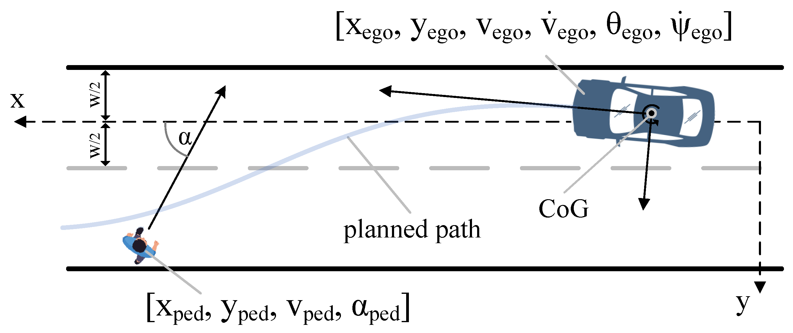
2.1. Problem Formulation

Our research fits into the hierarchical vehicle control structure shown in Figure 1. Global planning on the highest level defines the route based on road topology and traffic information. The next layer is behavior planning, which considers different scenarios, other traffic participants, and other factors. This layer can be considered as a state machine that covers all behaviors or actions: staying in the lane, following, avoiding, overtaking, and so on. The task of local planning is to design the trajectory or path associated with a behavior. Finally, the low-level controllers are responsible for executing the trajectory or path, whose outputs are the vehicle control commands. These layers can interact with each other, resulting in a replanning of the motion. For example, in a pedestrian avoidance case, the actual planned behavior and path are distracted by an unexpected object. Hence the vehicle needs to reconsider its strategy and defined trajectory.

This article focuses on local planning, which can consider several optimization factors. These are in priority order: safety, feasibility, perceived safety, comfort, and route efficiency. This optimization task needs to be solved with a high refresh rate and in real-time. Unfortunately, the resource requirements of classical nonlinear optimization methods can be high and cannot guarantee a constant run-time to achieve optimal results.

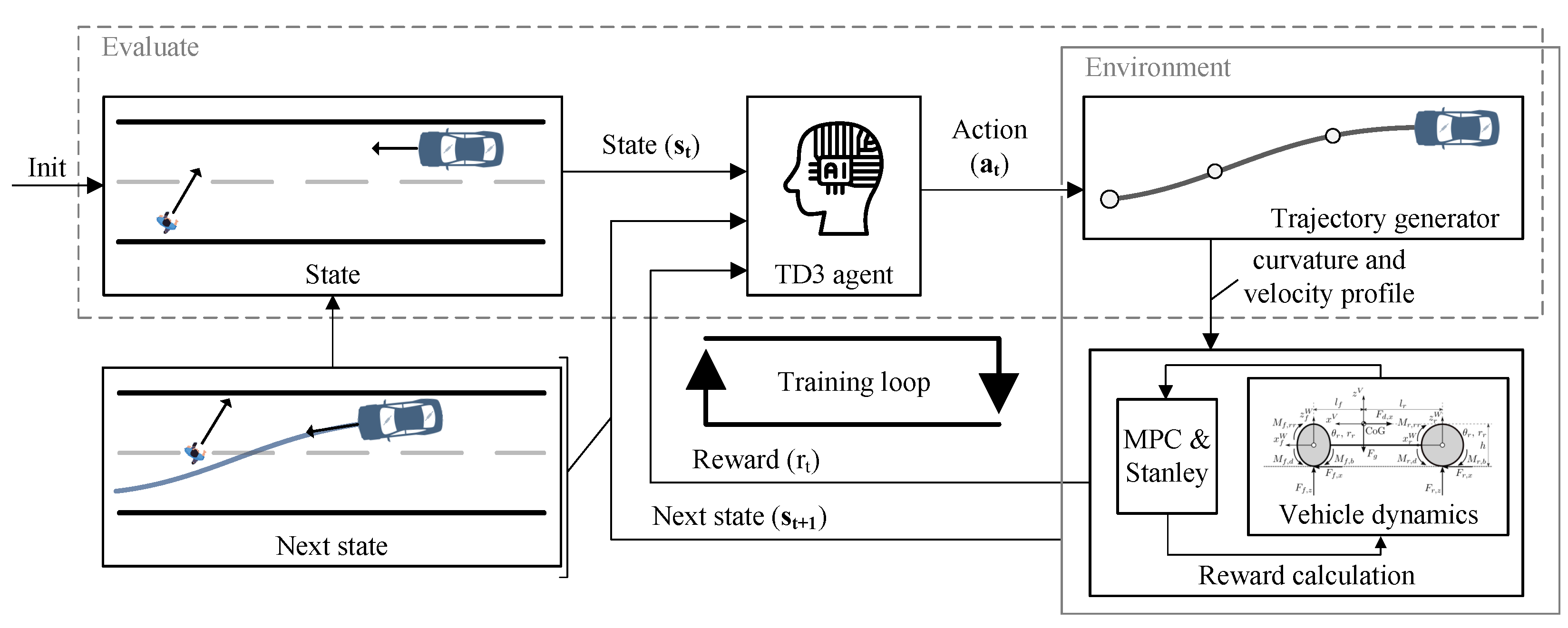
2.2. Proposed Method

The paper provides a machine learning-based solution for local planning to evade a moving object. A reinforcement learning agent achieves the optimization goal defined by the reward function in a learning environment through a trial and error method. In RL terminology, training consists of episodes, while episodes consist of a series of steps. The agent tries to solve a randomly generated scenario in each episode. Figure 2 shows the training method where the moving object is a pedestrian. The pedestrian’s starting position, velocity, direction, and EGO’s velocity are randomly generated when the scenario is initialized. The state space $s_t$ can be determined, from which the agent predicts the action space $a_t$. Based on the action space, the curvature and velocity profile of the trajectory can be generated.

A longitudinal Stanley and a lateral MPC controller drive along the entire trajectory while observing the vehicle and environmental conditions and calculating reward value $r_t$. In order to provide sufficiently accurate calculations of the vehicle dynamics with decent computational requirements, a nonlinear planar single-track vehicle model with a dynamic wheel model is applied. The vehicle executes only a $d{t}_{plan}$ length part of it. With this, the agent learns to look ahead. The performance of the trained agent can be examined in the evaluation phase.

The following simplifications were introduced at the beginning of the research to keep the problem in focus.

• The maneuver is performed on a straight section of the road.
• The vehicle has ideal high-level sensor signals.
• Constant road–tire friction coefficient.
• The pedestrian makes a rectilinear motion.
• No other dynamic objects are considered.

2.3. Environment

The training process can take up to million steps, so the balance between detail and run-time had to be found when creating the models and the reward function. The structure defined in Open-AI Gym was used as a basis to facilitate the integration of the agent. The problem presented in the article is numerically complex because the state and action space consist of several continuous values. The following subsections describe each of the software modules in the environment.

2.3.1. State Space

The state space consists of eight continuous variables. The first four describe the state of the pedestrian, and the others represent the vehicle’s state:

$$\begin{array}{cc}\hfill & [x_{ped}-x_{ego},y_{ped}-y_{ego},v_{ped},{\alpha }_{ped},v_{ego},{\dot{v}}_{ego},{\theta }_{ego},{\dot{\psi }}_{ego}],\hfill \end{array}$$

(1)

where $x_{ped}-x_{ego}$ and $y_{ped}-y_{ego}$ are the distance along the x and y axis between the EGO and the pedestrian, $v_{ped}$ is the velocity, and ${\alpha }_{ped}$ is the moving direction of the pedestrian. $v_{ego}$, ${\dot{v}}_{ego}$, ${\theta }_{ego}$, and ${\dot{\psi }}_{ego}$ are the velocity, acceleration, heading angle, and a yaw-rate of the EGO vehicle.

As shown in Figure 3, the origin of the global coordinate system is located on the centerline of the right lane, where the vehicle starts the episode with $v_0$ initial velocity. To improve the training stability of the agent, the elements of the state space are normalized to the range of $[0,1]$.

2.3.2. Action Space

The action space contains four continuous values. A curvature and a velocity profile define the agent’s planned trajectory.

As shown in Figure 4, a polynomial is defined by arc length and curvatures. As the agent provides curvature values, polynomial coefficients have to be calculated.

$$\kappa \left(s\right)=a_3{s}^3+a_2{s}^2+a_{1}s+a_0$$

(2)

The ${\kappa }_0$ curvature value at the beginning of the polynomial is equal to the coefficient $a_0$. According to ${\kappa }_1$, ${\kappa }_2$, and ${\kappa }_3$ the coefficients $a_1$, $a_2$, and $a_3$ are determined by analytical curve fitting. As Figure 4 shows, ${\kappa }_1$ and ${\kappa }_2$ are evenly distributed along the length of the polynomial in the middle. The curvature value at the end of the curve ${\kappa }_3$ is always 0.

The arc-length integral of the curvature function $\kappa \left(s\right)$ is $\theta \left(s\right)$ and its arc-length integral is the position $x\left(s\right)$, $y\left(s\right)$. $\theta \left(s\right)$ is the angle along the arc length, for which a numerical integration can provide a good approximation.

$$\theta \left(s\right)={\theta }_0+{\int }_0^s{a}_3{s}^{\prime 3}+a_2{s}^{\prime 2}+a_1{s}^{\prime }+a_{0}d{s}^{\prime }$$

(3)

$$x\left(s\right)=x_0+{\int }_0^{s}cos\left(\theta \left(s^{\prime }\right)\right)d{s}^{\prime }$$

(4)

$$y\left(s\right)=y_0+{\int }_0^{s}sin\left(\theta \left(s^{\prime }\right)\right)d{s}^{\prime }$$

(5)

The track points can be determined at a distance of 0.5 m along the arc length. The arc length s of a polynomial is velocity dependent. The planning horizon is 2 s.

The velocity profile is obtained by third-order B-spline interpolation. The first derivative at the beginning of the profile is equal to the current acceleration of the EGO. The curve’s control points are given by the second two continuous elements of the action space. These two velocity values are evenly distributed along the arc length.

2.3.3. Models

For accurate calculation of the vehicle’s motion with a fast run-time, a custom nonlinear single-track model with a dynamic wheel model is used [19]. Three elements build the multi-body model: the chassis and two rigidly connected virtual wheels. The main parameters of the chassis are the moment of inertia $\theta$, the mass m, the horizontal distance between the CoG and the wheel centers $l_f$ and $l_r$, the CoG’s height h, the moments of inertia ${\theta }_{[f/r]}$ and the radii $r_{[f/r]}$ of the wheels. The precisely developed wheel model uses the Magic Formula, which defines the transmittable amount of force between the road and the tires [20]. The vehicle model must be solved in ms time steps, which is the most resource-intensive part of the training due to the detailed wheel model. The pedestrian makes a rectilinear motion with the direction and speed specified at the beginning of the episode.

2.3.4. Reward Function

The reward function defines the goals of the agent. In other words, it gives the goodness of the actions represented by a single scalar value. In our case, the goal is to evade the pedestrian while maintaining the vehicle’s stability. The planned trajectory has to be evaluated to give feedback to the agent.

The primary optimization condition is to avoid a collision or minimize the collision’s severity if the collision is unavoidable. The non-slip maneuver and travel comfort are ranked lower in order of priority. The agent is penalized when the following terminating events occur, and the current episode is over:

• The euclidean distance between vehicle CoG and the nearest point of the path (distance error) greater than 1 m;
• The angle difference between at closest point of the path and vehicle (angle error) greater than 20 degrees;
• Longitudinal rear or front slip greater than 0.1;
• Lateral rear or front slip greater than 0.2 radians;
• The vehicle hit a pedestrian;
• The vehicle leaves the road.

The penalty is a linear function of the velocity, saturated at −2.5 to consider the severity of the caused accident in a simplified way:

$$r_t=max(-2.5;-2.5·v_{ego}/60)$$

(6)

where the $v_{ego}$ ego speed is in km/h. If the vehicle has accomplished the planned trajectory without a terminating event, the agent gets a weighted reward value:

$$r_t=w_v{r}_v+w_p{r}_p+w_{la}{r}_{la}+w_{lo}{r}_{lo}+w_a{r}_a$$

(7)

where $r_v$ is the reward of speed deviation from the velocity profile. $r_p$ penalizes the distance between EGO’s CoG and the centerline of the right lane. $r_{la}$ and $r_{lo}$ are the reward for the low lateral and longitudinal slip of the tires. $r_a$ penalizes the angle deviation of the road and the end of the trajectory. All of the reward values are saturated and normalized. $w_v$, $w_p$, $w_{la}$, $w_{lo}$, and $w_a$ are the weights. The maximum achievable reward value is 2.5.

2.3.5. Low-Level Controllers

As mentioned before, an MPC is responsible for the lateral, while a Stanley controller is responsible for the longitudinal control. Model predictive control can handle well the significant time delays of sensors or actuators and the high-order dynamics of vehicles, thus widespread in automotive applications [21]. During its operation, the MPC predicts the response of the process to the calculated control input with a dynamic model. The simplified two degrees of freedom model represented by the lateral position, and angle of rotation of the vehicle [22] has been integrated into the controller. For optimal control, a J cost function (8) is minimized using the control input.

$$J=\sum _{i=1}^p{W}_e{e}_i^2+\sum _{i=1}^p{W}_{\Delta u}\Delta u_i^2$$

(8)

where $e_i$ is the ith error between the reference value and the predicted output, p is the prediction horizon. The $W_e$ weight can specify the importance of reference tracking. $u_i$ is the ith control variable and $W_{\Delta u}$ weight can penalize significant changes in $u_i$. MPC calculates the best control input over the control horizon by minimizing the cost function at each timestep and defines the future plant output. The vehicle is controlled by the first calculated control signal in each time step. The controller can be tuned by adjusting the weighting coefficients, defining the sample time between predictions, and by the control horizon.

The longitudinal Stanley [23] is a simple proportional-integral (PI) controller where the integrator term is saturated to prevent windup:

$$u=(K_p+K_i{\displaystyle \frac{z}{z-1}})e$$

(9)

where u is the control signal, $K_p$ is the proportional gain, $K_i$ is the integral gain, and e is the difference between current and reference velocity. The control signal is also saturated.

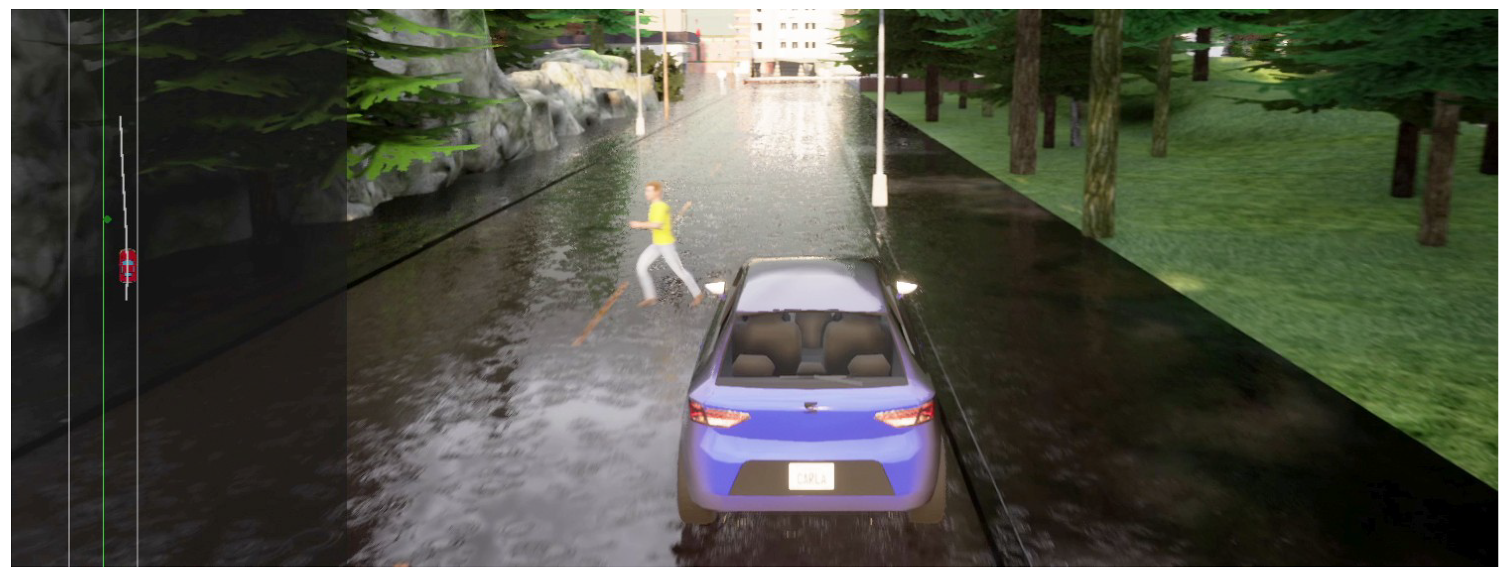
2.3.6. Rendering and Carla Integration

To facilitate the evaluation of the trained agent, a top-view 2D visualization interface has been integrated into the environment. Figure 5 shows a snapshot of the training that also shows the predicted position of the EGO and the pedestrian by the reward function.

In addition to the 2D display, a Carla 3D visualization (see Figure 6) has also been integrated with the environment for display purposes and to create a simulator environment for comparing the capabilities of human drivers to the performance of the RL.

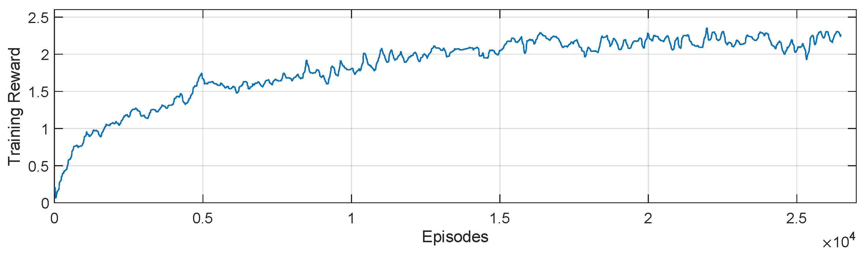
2.4. Agent

The RL agent uses the twin-delayed deep deterministic policy gradient (TD3) [24] algorithm, an improvement of the deep deterministic policy gradient (DDPG) [25]. DDPG can efficiently solve autonomous vehicle control tasks with a continuous state and action space [26,27]. Tuning hyperparameters (e.g., learning rate, noise process parameters, etc.) is challenging, especially for complex tasks with large action space.

In our previous work, the DDPG was detailed [26], hence in this article, the differences are in focus. TD3 has better performance due to three improvements.

• The overestimation can cause divergence in actor-critic solutions. As shown in

  Table 1. Hyperparameters of the training.

  Parameter	Value
  Soft-update parameter ($\tau$)	0.005
  Batch size	64
  Batch selection method	random choice
  Warmup steps	200
  Actor main, target networks
  Learning rate (${\alpha }_a$)	0.001
  Hidden F.C. layer structure	[512, 512, 4]
  Update steps	2
  Critic main, target networks
  Learning rate (${\alpha }_c$)	0.002
  Discount factor ($\gamma$)	0.99
  Hidden F.C. layer structure	[512, 512, 1]
  Action and Target-action noise
  Mean ($\mu$)	0.0
  Stddev ($\sigma$)	0.2
  Target action noise clip values	−0.5, 0.5

  TD3 updates the weights of the actor network only every second step. It can reduce the error, resulting in a more stable and efficient training process.
• TD3 agent uses two critic networks with a clipped double Q learning method [28]. The smaller worst of the two critic networks is selected, which reduces underestimation bias.
• The action noise regularization can smooth the target policy and make it more robust. As also shown in Table 1, saturated noise is added to the selected action, which favors higher values for the action.

Network Architecture and Hyperparameters

The tuning of the hyperparameters of the agent was done partly on a scientific basis and partly empirically. The agent uses two actor and four critic networks with the same layer structure. Table 1 shows that the networks consist of only a few layers with relatively few neurons, which is advantageous in terms of runtime, mainly for training but also for evaluation. The first two layers for both the actor and critic networks use the relu activation function. The activation function for the output layer of the critic is linear, and tanh for the actor. The target actor has saturated to a [0, 1] interval.

3. Results

The TD3 agent’s training results in a relatively small neural network using low resources. It can plan an optimal feasible trajectory for the vehicle based on its state and the dynamically moving object. Planning takes place online, and the trajectory is updated as the environment changes. As the car moves toward the pedestrian, it replans based on the changed state. On a medium-performance PC configuration (i7-7700 with GTX 1080 Ti), the agent learned in 26,464 episodes in 9 h and 24 min with randomized scenarios (see Figure 7). First, the vehicle starts on a straight track at a random speed. Then, the pedestrian appears in a randomized position and crosses the road at a random speed and direction. Noise is applied to the elements of the action space for exploration during training, according to Table 1.

An average driver rarely encounters dangerous traffic situations during their lifetime. Therefore, it is not easy to prepare for these situations. In addition to the vehicle’s type, equipment, and technical condition, much depends on the driver’s current condition and individual abilities to avoid or reduce the severity of the accident.

The performance of the trained agent was evaluated in comparison with human drivers. Eleven drivers with different qualifications participated in the research. The skills differed from not having a driving license to the one who was the driver for the Formula Student race team. The age distribution ranged from 25 to 45 years.

A simulation environment has been created to perform the tests, which consists of the following elements:

• Logitech G29 Racing wheel with force feedback;
• High-end PC with powerful graphics card (Nvidia 2080Ti);
• CARLA Simulator (version 0.9.13);
• The developed Python environment.

Table 2. Init parameters of the scenarios.

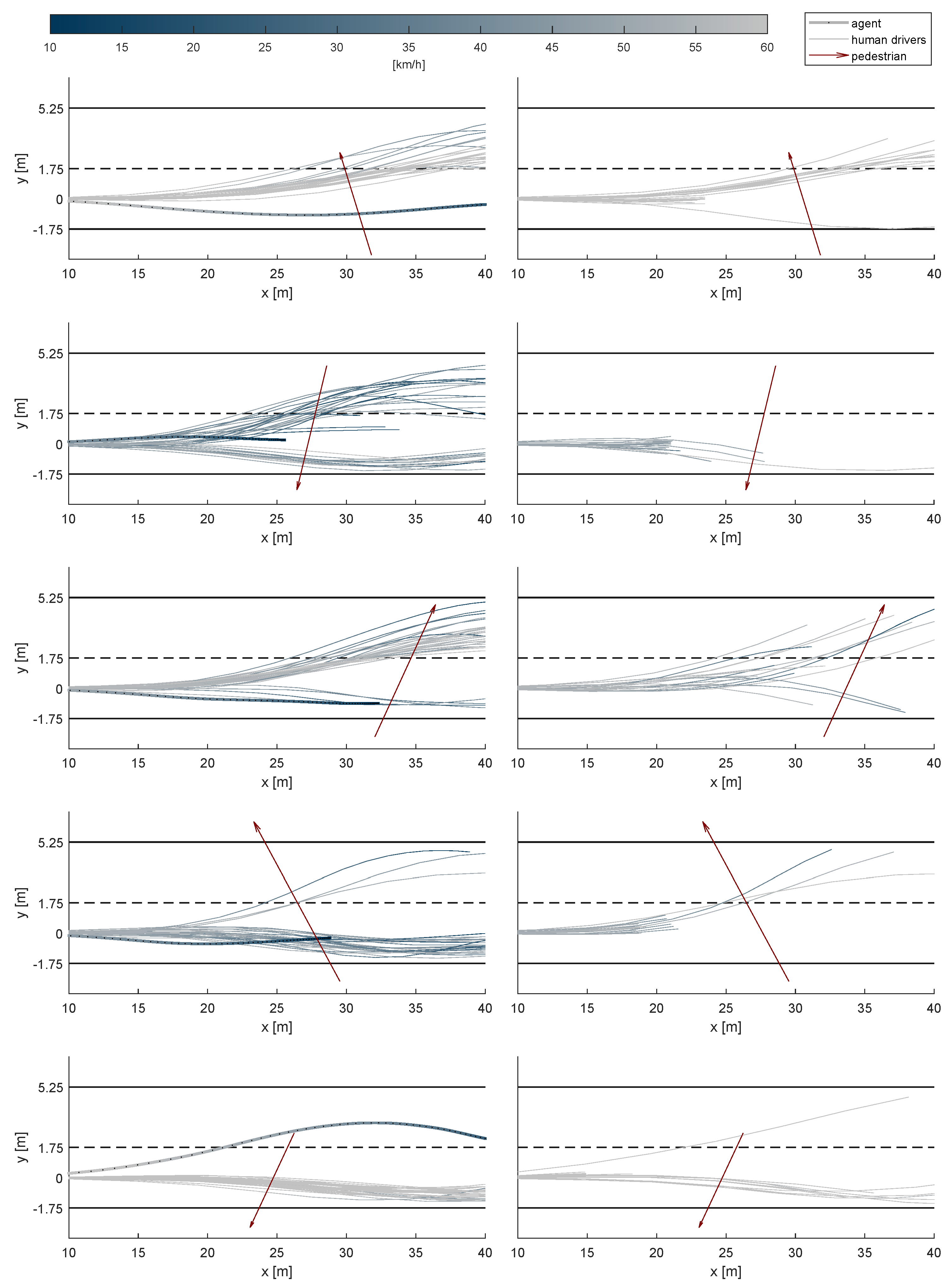
	Vehicle Speed (km/h)	Ped. Longitudinal Distace (m)	Ped. Velocity (km/h)	Ped. Moving Direction (°)
1	63.7	25.1	3.0	255.5
2	56.3	31.4	2.7	60.2
3	53.2	30.0	3.7	123.9
4	50.0	20.2	1.6	231.9
5	52.9	25.1	2.5	75.5
6	69.5	26.2	2.5	239.8
7	50.0	28.0	3.0	253.3
8	60.9	30.8	2.1	122.2
9	56.1	26.8	2.5	270.3
10	66.6	31.8	2.5	111.0

shows the randomly generated test cases, also known as scenarios, that had to be solved by drivers for five consecutive rounds. Each round contains ten scenarios, so one driver completed 50 runs. For the sake of comparability, all drivers perform the same scenarios.

The minimum speed of the vehicle at the beginning of the scenario was between 50 and 70 km/h. The pedestrians crossed the road at different angles, walking or running at different speeds, and started from different longitudinal distances (20–32 m) compared to the vehicle, resulting in a time-to-collision range of 1.4–2 s from the appearance of the pedestrian, making it quite challenging to sense, react, and avoid.

In all cases, the task of human drivers was to avoid an accident by steering and braking or accelerating, with a 3–5 s random time elapsing between each attempt, which simulates a surprising situation. Slightly wet asphalt was simulated during training for the agent to deal with more challenging conditions. The wheel–asphalt friction coefficient has been set to 0.7, significantly increasing the braking distance. Figure 6 shows that rainy weather was also set in the Carla for a more realistic simulation. As the focus of the research was not on creating highly accurate models, the vehicle model used in the tests and training did not include an electronic stability program (ESP). However, a simplified anti-lock braking logic was built into the model, which does not allow full locking even at maximum braking force for maneuverability. In addition, the steering ratio has been set lower than an average car, allowing faster steering response.

The agent completes all scenarios with a 100% success rate. A successful performance was defined as avoiding a collision and keeping the vehicle on the road in a controllable condition. The human drivers’ success is broken down into the scenarios and drivers, as shown in Figure 8 and

Table 3. Number of successful attempts of each driver on each scenario.

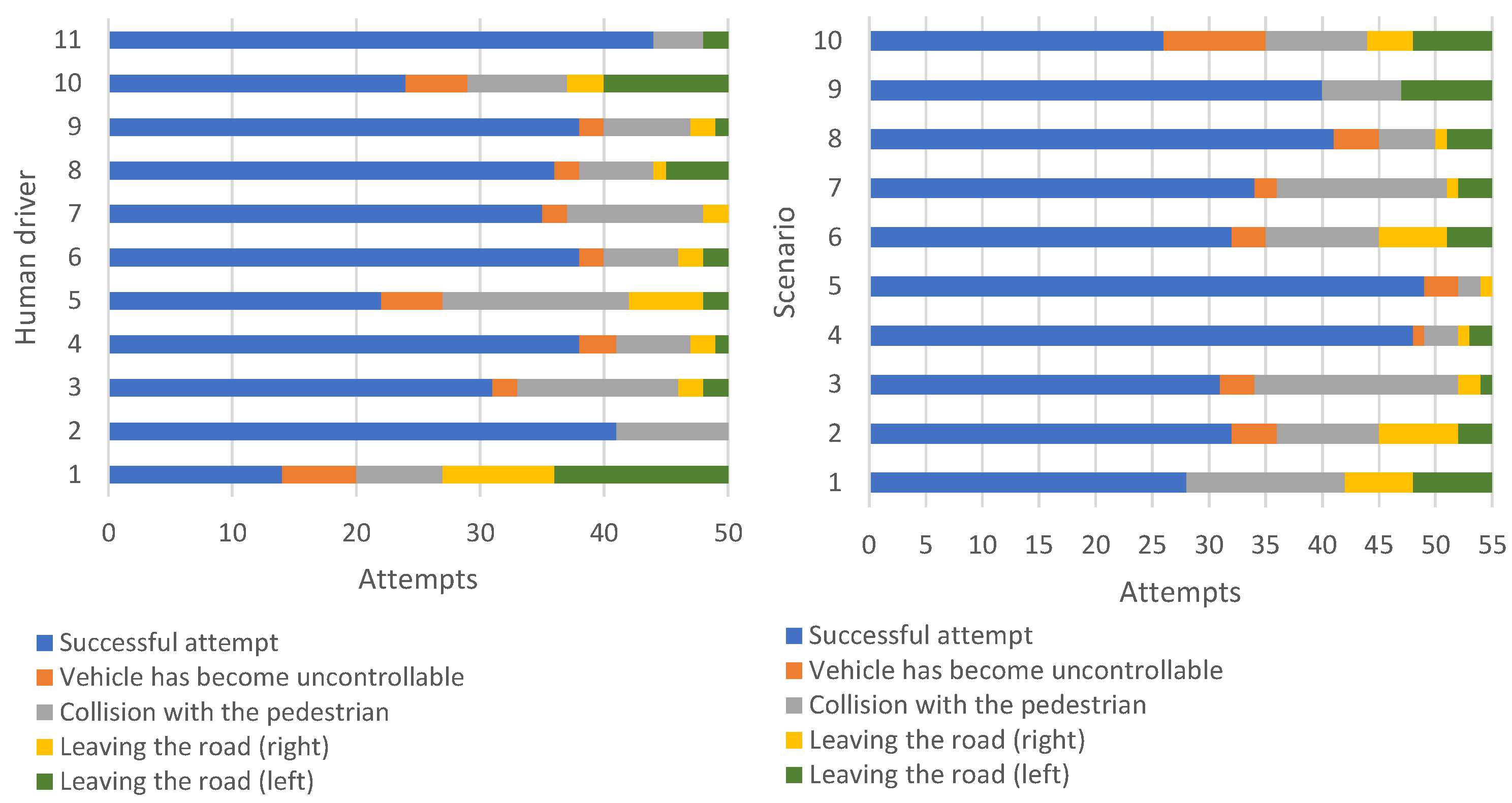
Human Drivers
		1	2	3	4	5	6	7	8	9	10	11	Sum
Scenarios	1	1	5	3	3	1	3	0	4	3	1	4	28
	2	1	4	2	3	2	3	3	4	4	1	5	32
	3	1	2	5	3	4	2	3	1	5	2	3	31
	4	2	5	3	5	4	5	5	5	5	4	5	48
	5	2	5	5	5	3	5	4	5	5	5	5	49
	6	2	5	2	4	1	4	2	2	3	3	4	32
	7	2	2	4	4	1	3	5	4	4	1	4	34
	8	2	5	3	4	3	4	5	5	3	2	5	41
	9	1	4	1	5	2	5	5	4	4	4	5	40
	10	0	4	3	2	1	4	3	2	2	1	4	26
	Sum	14	41	31	38	22	38	35	36	38	24	44

. The diagrams also show that there is also a difference between scenarios and drivers. Scenario 5 was the easiest, and it was successfully completed 49 times, while the 10th was the most difficult, and was only completed in half the attempts. The 11th driver was the most skillful with 44 successful attempts, while the first driver was the weakest. The majority of unsuccessful attempts are collisions with pedestrians. The second most common reason is to leave the road, and the third is to lose control of the vehicle. The drivers performed worst in the first round, though surprisingly, their performance fell after the third round. Their success rate for the individual rounds was 65%, 70%, 82%, 75%, and 69%, respectively.

In Figure 9 the diagrams from Scenarios 10, 7, 2, 3, and 6 are presented for a deeper understanding. The left columns show successful attempts (agent and humans), while the right ones provide the routes of unsuccessful attempts of the humans. Paths were given speed-dependent coloring according to the color bar, the faster the vehicle, the fainter the route. The path of the agent is marked with a thick line.

The drivers performed surprisingly well, but Figure 9 shows some critical differences. Human drivers rarely braked, while the agent applied high braking force in almost all cases, reducing the potential severity of the accident. In Scenarios 10 and 6, drivers chose a different strategy than the agent. In both cases, the human drivers drive at high speed in front of the pedestrian while the agent passes behind them more slowly. In Scenario 7, some human drivers pass in front of the pedestrian, while the others behind them only rarely brake. In Scenario 10, most incidents occurred when a pedestrian was passed, but finally, the vehicle became uncontrollable.

4. Conclusions

The paper presents an emergency pedestrian avoidance algorithm using reinforcement learning. Contrary to the end-to-end solutions found in the literature, it defines a path and a velocity profile to follow for the agent, which continuously replans its behavior based on the new state. In addition, the algorithm considers the severity, success, and controllability of the vehicle. Finally, we have compared the results to the capabilities of human drivers on the same simulation with the result that the agent can significantly outperform human performance. Though the algorithm presented is defined for Ackermann steering vehicles on the road with crossing pedestrians, one can apply its principles to various other dynamic object avoidance problems.

References

- Next Steps towards ‘Vision Zero’: EU Road Safety Policy Framework 2021–2030. Available online: https://op.europa.eu/en/publication-detail/-/publication/d7ee4b58-4bc5-11ea-8aa5-01aa75ed71a1 (accessed on 20 July 2022).
- Global Status Report on Road Safety 2018; World Health Organization: Geneva, Switzerland, 2018.
- Haus, S.H.; Sherony, R.; Gabler, H.C. Estimated benefit of automated emergency braking systems for vehicle–pedestrian crashes in the United States. Traffic Inj. Prev. 2019, 20, S171–S176. [Google Scholar] [CrossRef] [PubMed] [Green Version]
- Eckert, A.; Hartmann, B.; Sevenich, M.; Rieth, P. Emergency steer & brake assist: A systematic approach for system integration of two complementary driver assistance systems. In Proceedings of the 22nd International Technical Conference on the Enhanced Safety of Vehicles (ESV), Washington, DC, USA, 13–16 June 2011; pp. 13–16. [Google Scholar]
- Euro NCAP 2025 Roadmap; EuroNCAP: Leuven, Belgium, 2017.
- Borenstein, J.; Koren, Y. The vector field histogram-fast obstacle avoidance for mobile robots. IEEE Trans. Robot. Autom. 1991, 7, 278–288. [Google Scholar] [CrossRef] [Green Version]
- Fulgenzi, C.; Spalanzani, A.; Laugier, C. Dynamic Obstacle Avoidance in uncertain environment combining PVOs and Occupancy Grid. In Proceedings of the 2007 IEEE International Conference on Robotics and Automation, Roma, Italy, 10–14 April 2007; pp. 1610–1616. [Google Scholar] [CrossRef] [Green Version]
- Shimoda, S.; Kuroda, Y.; Iagnemma, K. Potential Field Navigation of High Speed Unmanned Ground Vehicles on Uneven Terrain. In Proceedings of the 2005 IEEE International Conference on Robotics and Automation, Barcelona, Spain, 18–22 April 2005; pp. 2828–2833. [Google Scholar] [CrossRef] [Green Version]
- Gelbal, S.Y.; Arslan, S.; Wang, H.; Aksun-Guvenc, B.; Guvenc, L. Elastic band based pedestrian collision avoidance using V2X communication. In Proceedings of the 2017 IEEE Intelligent Vehicles Symposium (IV), Los Angeles, CA, USA, 11–14 June 2017; pp. 270–276. [Google Scholar] [CrossRef]
- hwan Jeon, J.; Cowlagi, R.V.; Peters, S.C.; Karaman, S.; Frazzoli, E.; Tsiotras, P.; Iagnemma, K. Optimal motion planning with the half-car dynamical model for autonomous high-speed driving. In Proceedings of the 2013 American Control Conference, Washington, DC, USA, 17–19 June 2013; pp. 188–193. [Google Scholar] [CrossRef]
- Chen, Y.; Peng, H.; Grizzle, J.W. Fast Trajectory Planning and Robust Trajectory Tracking for Pedestrian Avoidance. IEEE Access 2017, 5, 9304–9317. [Google Scholar] [CrossRef]
- Wu, W.; Jia, H.; Luo, Q.; Wang, Z. Dynamic Path Planning for Autonomous Driving on Branch Streets With Crossing Pedestrian Avoidance Guidance. IEEE Access 2019, 7, 144720–144731. [Google Scholar] [CrossRef]
- Schratter, M.; Bouton, M.; Kochenderfer, M.J.; Watzenig, D. Pedestrian Collision Avoidance System for Scenarios with Occlusions. In Proceedings of the 2019 IEEE Intelligent Vehicles Symposium (IV), Paris, France, 9–12 June 2019; pp. 1054–1060. [Google Scholar] [CrossRef] [Green Version]
- Yoshimura, M.; Fujimoto, G.; Kaushik, A.; Padi, B.K.; Dennison, M.; Sood, I.; Sarkar, K.; Muneer, A.; More, A.; Tsuchiya, M.; et al. Autonomous Emergency Steering Using Deep Reinforcement Learning For Advanced Driver Assistance System. In Proceedings of the 2020 59th Annual Conference of the Society of Instrument and Control Engineers of Japan (SICE), Chiang Mai, Thailand, 23–26 September 2020; pp. 1115–1119. [Google Scholar] [CrossRef]
- Yang, J.; Xi, M.; Wen, J.; Li, Y.; Song, H.H. A digital twins enabled underwater intelligent internet vehicle path planning system via reinforcement learning and edge computing. Digit. Commun. Netw. 2022. [Google Scholar] [CrossRef]
- Deshpande, N.; Spalanzani, A. Deep Reinforcement Learning based Vehicle Navigation amongst pedestrians using a Grid-based state representation. In Proceedings of the 2019 IEEE Intelligent Transportation Systems Conference (ITSC), Auckland, NZ, USA, 27–30 October 2019; pp. 2081–2086. [Google Scholar] [CrossRef] [Green Version]
- Li, J.; Yao, L.; Xu, X.; Cheng, B.; Ren, J. Deep reinforcement learning for pedestrian collision avoidance and human-machine cooperative driving. Inf. Sci. 2020, 532, 110–124. [Google Scholar] [CrossRef]
- Everett, M.; Chen, Y.F.; How, J.P. Collision Avoidance in Pedestrian-Rich Environments with Deep Reinforcement Learning. IEEE Access 2021, 9, 10357–10377. [Google Scholar] [CrossRef]
- Hegedüs, F.; Bécsi, T.; Aradi, S.; Gáspár, P. Model Based Trajectory Planning for Highly Automated Road Vehicles. IFAC-PapersOnLine 2017, 50, 6958–6964. [Google Scholar] [CrossRef]
- Pacejka, H.B. Chapter 8—Applications of Transient Tire Models. In Tire and Vehicle Dynamics, 3rd ed.; Pacejka, H.B., Ed.; Butterworth-Heinemann: Oxford, UK, 2012; pp. 355–401. [Google Scholar] [CrossRef]
- Mehta, B.; Reddy, Y. Chapter 19—Advanced process control systems. In Industrial Process Automation Systems; Mehta, B., Reddy, Y., Eds.; Butterworth-Heinemann: Oxford, UK, 2015; pp. 547–557. [Google Scholar] [CrossRef]
- Rajamani, R. Vehicle Dynamics and Control; Springer: Berlin, Germany, 2012; p. 27. [Google Scholar] [CrossRef]
- Hoffmann, G.M.; Tomlin, C.J.; Montemerlo, M.; Thrun, S. Autonomous automobile trajectory tracking for off-road driving: Controller design, experimental validation and racing. In Proceedings of the 2007 American Control Conference, New York, NY, USA, 9–13 July 2007; pp. 2296–2301. [Google Scholar]
- Fujimoto, S.; van Hoof, H.; Meger, D. Addressing Function Approximation Error in Actor-Critic Methods. arXiv 2018, arXiv:1802.09477. [Google Scholar]
- Lillicrap, T.P.; Hunt, J.J.; Pritzel, A.; Heess, N.; Erez, T.; Tassa, Y.; Silver, D.; Wierstra, D. Continuous control with deep reinforcement learning. arXiv 2015, arXiv:1509.02971. [Google Scholar]
- Fehér, Á.; Aradi, S.; Bécsi, T. Hierarchical Evasive Path Planning Using Reinforcement Learning and Model Predictive Control. IEEE Access 2020, 8, 187470–187482. [Google Scholar] [CrossRef]
- Fehér, Á.; Aradi, S.; Hegedüs, F.; Bécsi, T.; Gáspár, P. Hybrid DDPG approach for vehicle motion planning. In Proceedings of the 16th International Conference on Informatics in Control, Automation and Robotics, ICINCO 2019, Prague, Czech Republic, 29–31 July 2019. [Google Scholar]
- Hasselt, H. Double Q-learning. Adv. Neural Inf. Process. Syst. 2010, 23, 2613–2621. [Google Scholar]