Abstract
Underwater target recognition is currently one of the hottest topics in computational intelligence research. However, underwater target recognition tasks based on deep learning techniques are difficult to conduct due to the shortage of acoustic echo signal samples, which results in poor training performance for existing deep learning models. Generative adversarial networks (GANs) have been widely used in data enhancement and image generation, providing a novel strategy for dealing with challenges in the research field mentioned above. To address the insufficiency of echo signal data for underwater high-speed vehicles, this paper proposes an underwater echo signal data enhancement method that uses an improved GAN based on convolution units for small sample sizes. First, we take pool test data as the training sample input and carry out data standardization, data interception, and copy-related processing work. Secondly, this paper proposes an improved generative adversarial network underwater (IGAN-UW) model to generate underwater echo signals. Finally, a CNN model combines the generated data with the original data to conduct classification training for underwater targets. Experimental results show that the IGAN-UW model is suitable for the generation of highly realistic original echo signals in cases with small sample sizes, providing a new approach to the active detection and recognition of underwater targets.
1. Introduction
Underwater high-speed vehicles are one of the main types of equipment used by ships, submarines, and aircraft for anti-submarine attacks in modern naval warfare. The underwater target recognition capability of these vehicles directly affects their hit probability and attack efficiency [1,2]. Target recognition capabilities are a significant indicator of an underwater high-speed vehicle’s overall performance and level of sophistication. Acoustic jamming equipment was initially limited to simulating the characteristics of point target and point source acoustic bait, but it has developed in recent years to include long-term array bait, two-dimensional planar array bait, and others. The traditional underwater target recognition method is based on the one-dimensional or two-dimensional scale characteristics of the target; this method is inadequate in the modern underwater battlefield full of new combat equipment. Traditional methods are now facing great challenges, and there is an urgent need to seek new approaches to feature extraction and target recognition [3,4,5].
Deep learning makes extensive use of data, and automatic learning is beneficial when representing classified features [6,7,8]. Deep learning is a machine learning technology that utilizes a multi-layer data processing network and has been widely applied in many areas, such as computer vision [9,10], speech recognition [11,12,13], natural language processing [14,15], remote sensing [16,17], and others. However, there are few works that study underwater target recognition based on deep learning techniques. In [18], principal component analysis (PCA) was used to identify the acoustic images of underwater targets, and the recognition rates were analyzed at various signal-to-noise ratios. Multiple features are extracted from interference images to create feature vectors, and feedforward neural networks are used to identify underwater targets [19]. The authors of [20] introduced the particle swarm optimization algorithm on top of the BP neural network to increase the network’s convergence speed and learning ability. However, obtaining underwater sample data for scientific research is extremely difficult due to environmental, time, and cost constraints. Inadequate sample sizes result in model training effectiveness being unsatisfactory [21]. Generative adversarial networks (GANs) have been widely applied in data enhancement [22,23,24,25], image generation [26,27,28], noise reduction in speech [29], and other applications. As a generative method, GANs can effectively address the problem of generating data. This is especially true for high-dimensional data because GANs do not limit the generation dimensions, which greatly broadens the range of the generated data samples. In addition, the adopted neural network structure can integrate different loss functions, which increases the flexibility of the design. The training process does not require the use of the inefficient Markov chain method or approximate inference, and there is no complex variational lower bound, which greatly improves the efficiency of training while decreasing its difficulty. Utilizing GANs to expand and enhance rare underwater target echo signal data can significantly enhance the training effectiveness of deep learning in the field of underwater recognition. However, the traditional GAN network model is incompatible with underwater echo samples from underwater high-speed vehicles and, thus, cannot be used to generate sample data directly. Traditional GANs are mainly aimed at high-dimensional data, such as images and videos. However, underwater echo signals are one-dimensional data. In addition, traditional GANs are designed for generating real-valued, continuous data and have difficulties directly generating sequences of discrete tokens. The reason for this is that, in GANs, the generator first starts with random sampling and then executes a deterministic transform governed by the model parameters. If the generated data are based on discrete tokens, the “slight change” guidance from the discriminative network makes little sense because there is probably no corresponding token for such a slight change in the limited dictionary space. As a result, it is a significant challenge to improve the GAN model for use with underwater echo samples.
To address the problem of insufficient underwater target data, this paper proposes an underwater echo signal data enhancement method based on an improved GAN for small sample sizes. First, we take pool test data as the training sample input and carry out data standardization, data interception, and copy-related processing work. Secondly, to solve the problem of insufficient underwater target data, this paper proposes an IGAN-UW model to generate underwater echo signal data under small-sample-size conditions. Finally, a convolutional neural network (CNN) model combines the generated data with the original data to conduct classification training for underwater targets [30,31,32,33]. Experimental results show that the IGAN-UW model proposed in this paper is suitable for the generation of highly realistic original echo signals in cases with small sample sizes, providing a new approach to the active detection and recognition of underwater targets.
2. Background
2.1. Traditional Underwater Target Recognition
In order to improve the survivability of naval vessels in the face of underwater high-speed vehicles, surface ships usually carry ‘soft-killing’ equipment, such as towed and assisted underwater acoustic decoys and underwater acoustic jammers to interfere with underwater high-speed vehicles attacking targets. Compared with naval vessels, submarines are mainly equipped with various types of “soft-kill” underwater combat equipment to improve their survivability. It can be predicted that the underwater combat environment, in the future, will be filled with various types of soft- and hard-killing devices, such as underwater acoustic decoys and jammers, and that the combat environment of underwater high-speed vehicles will be increasingly harsh.
As for underwater targets, the traditional recognition method is mainly based on target scale recognition technology. Target scale is one of the main characteristics of a target, and except for some underwater acoustic jamming devices with scale-simulation abilities, the size of most underwater acoustic decoys is much smaller than that of the actual target. Therefore, an important consideration for underwater target recognition is to make good use of the scale characteristics of the target.
From the perspective of underwater acoustic analysis, the vast majority of underwater acoustic interference devices can be regarded as point targets, and their target waveforms are as follows:
where is the signal envelope value of the point target, is the center frequency of the sonar transmitting signal, is the Doppler frequency shift of the simulated point target, is the time delay of the echo, and is the initial phase.
However, for large-size military targets, such as submarines, their horizontal size can be close to 100 m or longer, and they also have a huge vertical size. Such physical characteristics are often expressed using a multi-point model. Therefore, the real submarine target echo received by the homing system can be:
where N is the number of target bright spots, is the signal envelope of the th bright spot, is the time delay of the bright spot, and is the initial phase.
2.2. Generative Adversarial Network
A GAN is a game-theoretic generation model [34]. To be more specific, the model is capable of generating new samples with a probability distribution similar to that of the training samples through learning the probability distribution of the training samples. In this way, the model can accomplish the goal of data generation. This method has produced excellent results in a wide variety of research fields.
2.2.1. Network Structure
The fundamental structure of a GAN is depicted in Figure 1; it is primarily composed of two deep networks called generative and discriminant networks. The primary function of a generative network is to generate generated data that follow a specified distribution and are extremely similar to real data. The discriminant network’s primary function is to accurately distinguish real data from data generated by the generator [35,36].
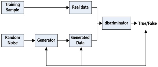
Figure 1.
Generative adversarial network structure diagram.
The learning process of a GAN can be described as a game in which the discriminator and generator constantly update and iterate their parameters to promote and improve one another. During this progress, the generator masters the skill of generating data that follows the same distribution as the real data. In the meantime, the discriminator develops a higher resolution due to continuous confrontation, which further improves the generated data’s quality.
2.2.2. Network Principle
The training process of GANs is essentially a game with the objective of convergence to the Nash Equilibrium. After training, generators learn the distribution of real data.
If the discriminant network is denoted by D and the generative network by G, the generated adversarial network’s loss function can be expressed as:
In Formula (1), X represents the input data of the discriminant network D, represents the probability that the discriminant network identifies the input data as real data, denotes the probability that the discriminant network identifies real data when the input is real data, and represents the probability that data are identified as generated data when the input is generated by the generating network. The loss function V(G, D) should be maximized when training the discriminant network. That is, when the input is real data from the training set, should be maximized; however, when the input is generated data from the generating network, should be minimized. The loss function V(G, D) must be minimized when training the generative network. Specifically, when the input is generated and the data are generated by the generative network, the maximum value of is obtained.
When generating an adversarial network for the purpose of training its corresponding discriminant network, the generator’s network parameters should be fixed, and only the discriminator’s network parameters should be updated. As a result of the loss Function (1), it is possible to deduce that the following equation should be maximized:
The extreme value problem denoted by Formula (2) can be solved by taking the derivative. Calculate the derivative of Formula (2) with respect to and set it to 0, and the corresponding maximum point can be obtained.
In the above formula, represents the point corresponding to the maximum value of the loss function (2), which can be obtained by substituting it into Formula (1).
In the above formula, represents the Kullback–Leibler divergence, which is mainly used to describe the differences between two steps [37]. denotes the Jensen–Shannon divergence (NCE), which is a deformation of the Kullback–Leibler divergence and has a greater capacity for discriminating between different distributions. The process of training the discriminator is essentially maximizing the Jensen–Shannon divergence [38].
Following that, when the generating adversarial network trains its corresponding generating network, the generating network’s network parameters are updated when the discriminator achieves the maximum Jensen–Shannon divergence so that the Jensen–Shannon divergence between the probability step of generating and discriminating data is minimized, i.e.,
When the above formula reaches its minimum value, must reach the minimum value. That is, the difference in probability distributions between real data and generated data should be as small as possible.
3. Methodology
3.1. Underwater Target Water Wave Data Processing
In this paper, the beam output signal of the underwater target echo received by the active detection systems of underwater high-speed vehicles in the pool test data is taken as the basis and then processed as the training sample input. There are two primary reasons for not directly feeding the neural network the output data from the original beam. First, the original signal’s weak target characteristics would increase the difficulty of training the network. To be more specific, a weak target means that the target signal is weak, the signal-to-noise ratio is low, and it is not easy to detect. The weak target characteristics of the original signal not only easily lead to the problem of high missed detection rates using the mainstream signal detection methods but also lead to corresponding signal characteristics that are easily affected by background and noise, resulting in problems such as identification difficulties. In addition, the weak target characteristics of the original beam lead to the problem that a target whose spectral energy is less than the noise is smoothed, which ultimately leads to the target being unable to be effectively detected. Therefore, using output data from the original beam makes network training more difficult. Second, because of the large dimension of the original signal’s sample, there would be an excessive number of network training parameters and an exponential increase in the amount of calculation required. A multi-dimensional disaster would occur due to such a huge increase in the pressure on the computer. This paper aims to perform data standardization, data interception, and copy-related processing on the original echo data to reduce the data dimension and enhance the target features for application to the neural network model. Figure 2 illustrates the signal processing process.
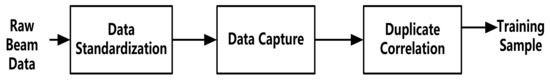
Figure 2.
Data processing flow.
First, the data are standardized. Because each sample has a unique distribution range due to the varied experimental conditions, the data must be processed in a standardized manner. This paper uses the Z−Score standardization method to achieve data standardization. The data are transformed into the same scale by first removing the mean value and then dividing it by the standard deviation, as shown in the following formula:
where is the mean value of this feature, and is the standard deviation. The mean value of the standardized sample data is 0, the variance is 1, and it is dimensionless.
The data are then intercepted. As the echo data received by the active acoustic detection system of an underwater high-speed vehicle can be as long as tens or hundreds of thousands of points in a single cycle, and the target distance constantly changes with each detection cycle, the length of the received signal varies with each cycle. Generally, the length of the echo data varies. As a result, it is necessary to intercept the original echo signal and concentrate on the data collected in the energy-gathering area of the target echo to reduce the dimension of the input data and improve the model’s training efficiency.
Finally, copy correlation is used to process the data. Due to the significant effect of background interference on the intercepted data samples, their features are not prominent enough, and there is little difference between different samples. It is necessary to perform duplicate correlation processing on the data. Copy correlation is primarily accomplished by using a cross-correlation receiver, which effectively increases the signal-to-noise ratio of echo data and highlights target features, as illustrated in Figure 3.
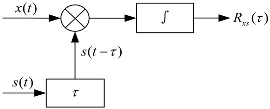
Figure 3.
Correlation machine receiving principle.
In Figure 3, x(t) denotes the signal received by sonar, s(t) represents the reference signal (the copy of the signal transmitted by sonar is generally taken), is the signal delay time, and the output is the cross-correlation function. When the signal delay time is equal to the time delay of the target echo, the cross-correlation function can obtain the maximum value, referred to as the copy correlation peak.
In this paper, according to actual engineering experience, data interception and copy-related processing are performed on the normalized original data of the pool experiment, yielding a sample with a length of 1024 data points. As illustrated in Figure 4, a certain segment of the echo signal is randomly selected, and the time domain waveforms before and after data processing are compared. Compared with the original echo signal, the dimension of the processed echo signal data is greatly reduced, and the signal-to-mix ratio and data quality are significantly improved. After processing, the data set of this paper contains 288 samples, each of which contains 1024 data points.
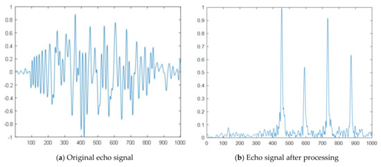
Figure 4.
Echo signal before and after processing.
3.2. Framework of Underwater Target Recognition Based on the GAN
As shown in Figure 5, based on the original underwater acoustic target samples obtained in the pool test, this paper designs an underwater target recognition neural network modeling scheme based on IGAN-UV. Based on the original target data, the copy-correlated samples with one-dimensional characteristics are obtained. Due to the insufficient amount of original data, the sample size of the copy-correlated data obtained is insufficient to support neural network training, and the result is not ideal. Therefore, the sample size is expanded using the GAN network. Based on the expanded underwater target sample set, a convolutional neural network model is established to classify and verify the underwater acoustic data samples. For copy-correlated samples, operations such as convolution and pooling in the common convolutional neural network can be transformed into n*1 to adapt to sample characteristics.
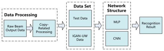
Figure 5.
Neural network modeling scheme.
The convolutional neural network model must consider the influence of parameters such as the convolution kernel, the size of the pooling window, and the step size; it must also constantly adjust all kinds of data and, finally, determine the grid structure suitable for the underwater target echo. Since the copy-correlated sample data in this paper are mainly one-dimensional, this section only describes the one-dimensional convolutional neural network modeling scheme for copy-correlated sample data in the experiment.
In the modeling process, this paper uses the classical structure of convolution and pooling alternating with each other. The pooling layer structure is relatively simple, and the main question is how to determine the convolution structure. In combination with the common form of convolution kernels and the sample length used, this paper conducts repeated experimental comparisons among several convolution kernels and chooses the average pooling mode. To correspond to the cost function selected in this paper, the Softmax classifier is taken as the output layer, and the node of the output layer is 3.
After experimental comparisons, the final detailed grid parameters of the one-dimensional convolutional neural network model are as shown in the following Table 1.

Table 1.
Structure of CNN Model.
This network structure firstly uses convolution and pooling operations to process and analyze features; this can be regarded as a method of feature engineering. The full-connection layer connects all feature maps and, finally, the Softmax layer is introduced to classify data.
3.3. IGAN-UW for Underwater Target Recognition
3.3.1. Structural Design of the Network
The network structure for generating countermeasure models is designed for the specific task of generating echo signals for underwater targets with a small sample size.
In contrast to the traditional image generation task (which uses a two-dimensional matrix as the training sample), the sample for the echo signal generation task uses a one-dimensional vector. As a result, the GAN’s fundamental unit should be a full connection layer or a one-dimensional convolution layer. The convolutional structure has the characteristics of a local sensing field and weight sharing; this not only reduces the number of parameters and the complexity of the network model but also ensures invariance at large scales and translations, making it widely applicable. As a result, this paper chooses a one-dimensional convolutional structure as the primary operating unit of the GAN. A GAN is composed of two modules: a generative network and a discriminant network. The generated network’s detailed structure is illustrated in Figure 6, where deconv denotes the deconvolution layer, stride denotes the step size, filters denote the number of channels in the convolutional core, BatchNorm denotes batch normalization, and activation denotes the activation function. The generative network is composed primarily of three layers: an input layer, an output layer, and five deconvolution units. To avoid the gradient disappearing, the leaky ReLU function is chosen as the activation function of the first four deconvolution units; the tanh function is chosen as the activation function of the fifth deconvolution unit to ensure that the output is between −1 and +1. Additionally, batch normalization is applied to the first four deconvolution units to accelerate convergence and avoid over-fitting.
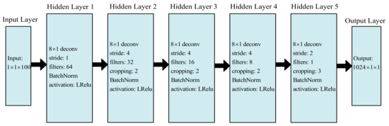
Figure 6.
Detailed structure diagram of the generative network.
The discriminant network’s detailed structure is depicted in Figure 7, where conv denotes the convolution layer and the label Fully Connected represents the fully connected layer. Discriminant networks are composed of an input layer, an output layer, three convolution units, and a fully connected layer. Similarly, the leaky ReLU activation function is chosen for the three convolutional units and the fully connected layer to avoid gradient disappearance; batch normalization is also added to the three convolutional units to improve convergence and avoid over-fitting.
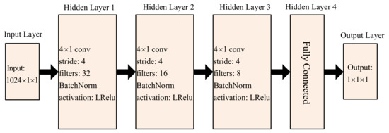
Figure 7.
Detailed structure diagram of the discriminative network.
First, the generative network is fed random noise with a length of 100 data points. The generated signal with a length of 1024 data points is output after five deconvolution units. The generated and real signals are then fed into the discriminant network. The true and false information for the signal is finally output after three convolution units and a full connection layer with a total of 128 neurons.
3.3.2. Training Process
Figure 4 illustrates the training process for GANs. The training procedure for this network is detailed below.
- Train the generated network. A generated network (generator) tries its best to generate false pictures that are approximately true from random noise. As illustrated in Figure 8, the discriminant network’s parameter training process is frozen, and only the generated network is updated (a). The generated network’s input is random noise, and its label is true (1). The output is either true or false information (0/1); to be more specific, the generator generates a false signal, sends it to the discriminator, and trains the generator according to the determination result (note that the parameters of the discriminator should not be updated at this time);
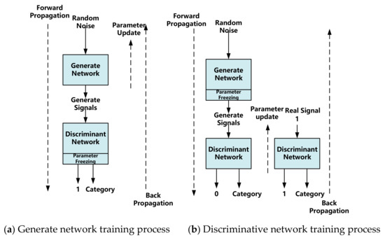 Figure 8. Schematic diagram of the GAN training process.
 - Train the discriminant network. A discriminant network (decision maker) tries its best to distinguish between real pictures and false signals (signals generated by the generator). The parameters of the generated network are frozen, and only the discriminant network’s parameter training process is updated, as illustrated in Figure 8b. A discriminant network has two types of input. One is the signal generated by random noise passing through the generated network, and its associated label is false (0). One is a real signal, and the label to which it corresponds is real (1). The output is either true or false information (0/1). To be more specific: first, send a real signal to the discriminator, mark the sample as true, and train the discriminator; second, the generator generates a false signal, sends it to the discriminator, marks the sample as false, and trains the discriminator;
- Repeat steps 1 and 2 in sequence until convergence occurs. The generated signal becomes increasingly close to the real signal through continuous confrontation between the generated network and the discriminant network.
In summary, the GAN training process is as follows:
- (1)
- Randomly sample the noise data distribution, input the generation model, and obtain a set of false data, which is recorded as D(z);
- (2)
- Randomly sample the distribution of real data as real data and record it as X;
- (3)
- Take the data generated in one of the first two steps as the input of the discrimination network (so the input of the discrimination model is two types of data: true/false), and the output value of the discrimination network is the probability that the input belongs to the real data. Real is 1, and fake is 0;
- (4)
- Then, calculate the loss function according to the obtained probability value;
- (5)
- According to the loss function of the discriminant model and the generated model, the parameters of the model can be updated by using the back propagation algorithm. (First, update the parameters of the discrimination model, and then update the parameters of the generator through the noise data obtained by resampling).
The GAN network trains the generation model through the training set, and its corresponding verifier samples train the discrimination model. A new test set is used to test the model generated by the GAN network, and the final results are obtained.
4. Experimental Verification and Result Analysis
4.1. Experimental Data
The underwater echo data used in this paper are all from experimental tests conducted at the anechoic pool at the Xi’an Institute of Precision Mechanics. Figure 9 illustrates the experimental platform, with the Key Laboratory of Underwater Information and Control in Figure 9a, and the anechoic pool in Figure 9b.
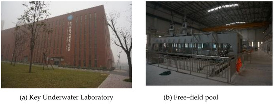
Figure 9.
Experimental platform.
Using the principal prototype of an underwater high-speed vehicle homing system, a hard-in-the-loop simulation environment for underwater targets is constructed based on the actual application environment and situation of underwater high-speed vehicles. Figure 10 depicts the pool experiment. When the underwater high-speed vehicle moves in the direction of the underwater target, it emits detection signals that are reflected by the target and converted to echo signals by the underwater high-speed vehicle’s detection system.
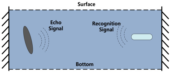
Figure 10.
Side view of pool experiment.
4.2. IGAN-UW Experimental Verification and Analysis
To validate the effectiveness of the target echo signal generation model proposed in this paper, the target echo signal processed in Section 3.1 is used as the real signal for the echo signal generation experiment. Table 2 summarizes the hyperparameters used in model generation training.
Table 2.
Training super parameter selection.
The optimizer used in this paper for network model training is the Adam function, which has a high convergence rate in deep learning. To prevent the network from over-fitting, L2 regularization with a coefficient of 0.001 is applied. Due to the small size of the training set, this paper chooses small batches for training and sets the batch size to 4, ensuring that the network parameters are updated 72 times in each round.
The number of rounds of network training affects the quality of the generated signals. An insufficient number of rounds results in under-fitting, resulting in a significant difference between the generated and pool test signals. An excessive number of training rounds results in over-fitting and causes the generated signal to converge with the pool test signal in the pool, which could weaken the significance of the generated signal. The generated signals and their associated amplitude probability distributions are compared below for 100, 150, 200, and 250 rounds of training.
After 100 rounds of training, Figure 11 compares the generated signals with the pool test signals. Figure 11a depicts the waveforms of 16 randomly selected test signals. Figure 11b depicts the waveforms of 16 randomly generated signals. The amplitude probability distributions of the test signals and generated signals from 288 pools are compared in Figure 11c. It can be seen in the figure that after 100 epochs of training, the generated signals from a subset of the 16 random signals gradually maintain a shape similar to that of the pool test signals. The amplitude probability distributions of the signals show that the generated signals appear to be close to the shape of the distribution of the pool test signals.
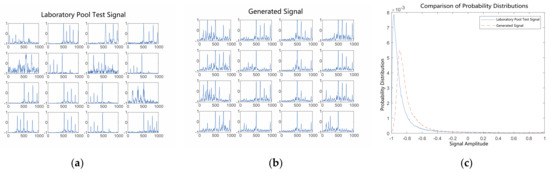
Figure 11.
Comparison of generated signals with pool test signals after 100 epochs of training. (a) Laboratory pool test signals. (b) Generated signals. (c) Probability distributions of signal amplitudes.
After 150 rounds of training, Figure 12 compares the generated signals with the pool test signals. The waveforms of the generated signals show that the distribution of highlights in the generated signals is relatively chaotic in terms of the number of highlights. The signals generated after 150 rounds of training were slightly sharper than those generated after 100 rounds in terms of the signal amplitude probability distributions; however, the probability distributions of both remained basically the same. This indicates that the proposed method hopefully converges to the optimal situation as the number of training epochs increases.
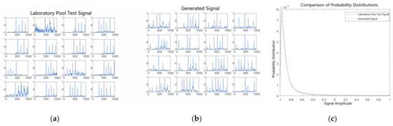
Figure 12.
Comparison of generated signals with pool test signals after 150 epochs of training. (a) Laboratory pool test signals. (b) Generated signals. (c) Probability distributions of signal amplitudes.
After 200 rounds of training, Figure 13 compares the generated signals with the pool test signals. Similarly, from a signal waveform perspective, the generated signals’ equal interval distributions are consistent with those of the pool test signals, and the number of highlights is consistent with the pool test signals between 3 and 6. In terms of the signal amplitude probability density distributions, the trends of the generated signals’ and pool test signals’ amplitude probability density distributions are essentially consistent. This demonstrates that the proposed method has mostly converged at this point.
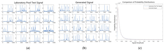
Figure 13.
Comparison of generated signals with pool test signals after 200 epochs of training. (a) Laboratory pool test signals. (b) Generated signals. (c) Probability distributions of signal amplitudes.
After 250 rounds of training, Figure 14 compares the generated signals with the pool test signals. In terms of the signal waveform level, the generated signals’ equal interval distributions are basically consistent with those of the pool test signals, and the number of highlights is basically consistent with the pool test signals between 3 and 6. However, as indicated by the signal amplitude probability density distributions, the gap between the generated and pool test signals begins to widen, indicating that too many training rounds result in over-fitting and the loss of meaning for the generated signals.
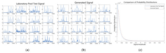
Figure 14.
Comparison of generated signals with pool test signals after 250 epochs of training. (a) Laboratory pool test signals. (b) Generated signals. (c) Probability distributions of signal amplitudes.
As can be observed from the above training process, the proposed model achieves the best results around 200 epochs. The generated echo signal is basically consistent with the pool test signal in terms of signal waveform and amplitude probability density distribution. Although the inevitable tendency toward over-fitting gradually appears as the number of training epochs increases, the model still shows a favorable optimization result.
4.3. Recognition of Experimental Verification and Analysis Based on a CNN Model
In order to accelerate the convergence of the model, a BN layer is added after each convolution layer for a CNN model with a one-dimensional time series. In addition, in order to ensure the generalization ability of the model, regularization is conducted by using the dropout strategy before the classification layer, and the probability coefficient is set to 0.4. The Adam algorithm is also used to update the parameters of the network, and the initial learning rate is set to 0.001. Every 15 epochs, the process is attenuated to half of the original, and the training process is stopped after 75 epochs.
As can be seen in Table 3, the proposed method obtains the best recognition rate for the line target. However, the recognition rate of the point target is not satisfactory.
Table 3.
Comparison of target recognition rate using different samples.
After the underwater target sample set is expanded by the IGAN-UW, neural network training is conducted again, and the results of the different samples obtained are shown in Table 4. At the same time, the MLP model is added for comparison. Some information can be obtained from the table. First, after data enhancement, the proposed method obtains 4% and 35.5% improvements in the recognition rates of the body target and point target, respectively. Although the recognition rate of line targets does not improve, the overall average recognition rate improves by 13.4%. Second, it can be clearly seen that the proposed model obtains a nearly 1.58-times improvement in the point target recognition rate after data enhancement. Finally, as a comparison, the MLP-based approach also obtains a good improvement in the target recognition rate after data enhancement; however, the proposed model consistently maintains better performance, both before and after the enhancement. The results show that the enhanced data of the IGAN-UW model can largely solve the problem of insufficient underwater target sample sizes by expanding the existing data set and effectively improving the underwater target identification ability of the model.
Table 4.
Comparison of data enhancement results.
4.4. Discussion
One of the trendiest issues in contemporary computational intelligence research is underwater target recognition. Here, the processed target echo signal is used as the actual signal for the echo signal generation experiment in order to verify the efficacy of the target echo signal generating model proposed in this study. As shown in the experiments, the quantity of network training cycles has an impact on the output signal’s quality. Inadequate rounds lead to under-fitting. The generated signal becomes identical to that of the pool test signal if there are too many rounds, which causes over-fitting and renders the created signal meaningless. In the recognition experiments, for the CNN model with a one-dimensional time series, a BN layer is added following each convolution layer to quicken the model’s convergence. The results demonstrate that the IGAN-UW model’s enhanced data may significantly reduce the issues caused by small underwater target sample sizes by enlarging the existing data set and significantly increasing the model’s capability to identify underwater targets.
5. Conclusions
To address the issue of insufficient underwater target echo signal data and high acquisition costs, this paper proposes a method for enhancing underwater high-speed vehicle echo signal data using a generative countermeasure network under small-sample-size conditions. Combined with the echo signal’s characteristics, an IGAN-UW model based on convolutional units is designed and constructed. Finally, the generated signal’s validity is verified at the signal waveform and amplitude probability distribution levels. The experimental results demonstrate that the proposed model can effectively generate highly realistic echo signals, even with small sample sizes, which introduces a novel concept for underwater target detection and recognition. The IGAN-UW network proposed in this paper is based on underwater echo signals with small sample sizes, and the generated data lacks classification information. The expanded underwater target echo data set based on the IGAN-UW model uses a CNN model for target recognition and classification, which effectively improves the underwater target recognition effect and provides a new method for underwater target recognition.
Author Contributions
Conceptualization, Z.W.; Data curation, C.W.; Formal analysis, J.D.; Investigation, Y.Y.; Methodology, L.L.; Resources, K.Z.; Software, J.Z. All authors have read and agreed to the published version of the manuscript.
Funding
This work was supported by the Natural Science Basic Research Plan in Shaanxi Province of China [grant number 2022JQ-671] and the 68th Batch of China Postdoctoral Foundation [grant number 2020M683597].
Institutional Review Board Statement
Not applicable.
Informed Consent Statement
Not applicable.
Data Availability Statement
Not applicable.
Acknowledgments
The authors appreciate the linguistic assistance from Li Hao during the revision of this paper.
Conflicts of Interest
The authors declare no conflict of interest.
References
- Chen, L.; Zheng, M.; Duan, S.; Luo, W.; Yao, L. Underwater Target Recognition Based on Improved YOLOv4 Neural Network. Electronics 2021, 10, 1634. [Google Scholar] [CrossRef]
- Kamal, S.; Mohammed, S.K.; Pillai, P.R.S.; Supriya, M.H. Deep learning architectures for underwater target recognition. Ocean. Electron. 2013, 48–54. [Google Scholar]
- Jiang, X.-D.; Yang, D.-S.; Shi, S.-G.; Li, S.-C. The research on high speed underwater target recognition based on fuzzy logic inference. J. Mar. Sci. Appl. 2006, 5, 19–23. [Google Scholar] [CrossRef]
- Jiang, J.; Wu, Z.; Lu, J.; Huang, M.; Xiao, Z. Interpretable features for underwater acoustic target recognition. Measurement 2021, 173, 108586. [Google Scholar] [CrossRef]
- Liu, J.; Gong, S.; Guan, W.; Li, B.; Li, H.; Liu, J. Tracking and Localization based on Multi-angle Vision for Underwater Target. Electronics 2020, 9, 1871. [Google Scholar] [CrossRef]
- LeCun, Y.; Bengio, Y.; Hinton, G. Deep learning. Nature 2015, 521, 436–444. [Google Scholar] [CrossRef]
- Guo, Y.; Liu, Y.; Oerlemans, A.; Lao, S.; Wu, S.; Lew, M.S. Deep learning for visual understanding: A review. Neurocomputing 2016, 187, 27–48. [Google Scholar] [CrossRef]
- Teng, B.; Zhao, H. Underwater target recognition methods based on the framework of deep learning: A survey. Int. J. Adv. Robot. Syst. 2020, 17. [Google Scholar] [CrossRef]
- He, K.; Zhang, X.; Ren, S.; Sun, J. Spatial pyramid pooling in deep convolutional networks for visual recognition. IEEE Trans. Pattern Anal. Mach. Intell. 2015, 37, 1904–1916. [Google Scholar] [CrossRef] [Green Version]
- Li, H.; Li, J.; Zhao, Y.; Gong, M.; Zhang, Y.; Liu, T. Cost-Sensitive Self-Paced Learning with Adaptive Regularization for Classification of Image Time Series. IEEE J. Sel. Top. Appl. Earth Obs. Remote Sens. 2021, 14, 11713–11727. [Google Scholar] [CrossRef]
- Rahmani, M.H.; Almasganj, F.; Seyyedsalehi, S.A. Audio-visual feature fusion via deep neural networks for automatic speech recognition. Digit. Signal Process. 2018, 82, 54–63. [Google Scholar] [CrossRef]
- McLaren, M.; Lei, Y.; Scheffer, N.; Ferrer, L. Application of convolutional neural networks to speaker recognition in noisy conditions. In Proceedings of the Fifteenth Annual Conference of the International Speech Communication Association, Singapore, 14–18 September 2014. [Google Scholar]
- Zhang, Z.; Geiger, J.; Pohjalainen, J.; Mousa, A.E.; Jin, W.; Schuller, B. Deep learning for environmentally robust speech recognition: An overview of recent developments. ACM Trans. Intell. Syst. Technol. (TIST) 2018, 9, 1–28. [Google Scholar] [CrossRef]
- Zhang, Y.; Marshall, I.; Wallace, B.C. Rationale-augmented convolutional neural networks for text classification. In Proceedings of the Conference on Empirical Methods in Natural Language Processing, Austin, TX, USA, 16–20 November 2016; p. 795. [Google Scholar]
- Mirończuk, M.M.; Protasiewicz, J. A recent overview of the state-of-the-art elements of text classification. Expert Syst. Appl. 2018, 106, 36–54. [Google Scholar] [CrossRef]
- Li, H.; Gong, M.; Wang, C.; Miao, Q. Self-paced stacked denoising autoencoders based on differential evolution for change detection. Appl. Soft Comput. 2018, 71, 698–714. [Google Scholar] [CrossRef]
- Li, H.; Gong, M.; Zhang, M.; Wu, Y. Spatially self-paced convolutional networks for change detection in heterogeneous images. IEEE J. Sel. Top. Appl. Earth Obs. Remote Sens. 2021, 14, 4966–4979. [Google Scholar] [CrossRef]
- Xu, J.; Bi, P.; Du, X.; Li, J.; Chen, N. Generalized robust PCA: A new distance metric method for underwater target recognition. IEEE Access 2019, 7, 51952–51964. [Google Scholar] [CrossRef]
- Zhang, Q.; Da, L.; Zhang, Y.; Hu, Y. Integrated Neural Networks based on Feature Fusion for Underwater Target Recognition. Appl. Acoust. 2021, 182, 108261. [Google Scholar] [CrossRef]
- Wang, X.; Wang, G.; Wu, Y. An adaptive particle swarm optimization for underwater target tracking in forward looking sonar image sequences. IEEE Access 2018, 6, 46833–46843. [Google Scholar] [CrossRef]
- Cao, X.; Zhang, X.; Yu, Y.; Niu, L. Deep learning-based recognition of underwater target. In Proceedings of the IEEE International Conference on Digital Signal Processing (DSP), Beijing, China, 16–18 October 2016; pp. 89–93. [Google Scholar]
- Wang, J.; Chen, Y.; Gu, Y.; Xiao, Y.; Pan, H. SensoryGANs: An effective generative adversarial framework for sensor-based human activity recognition. In Proceedings of the International Joint Conference on Neural Networks (IJCNN), Rio de Janeiro, Brazil, 8–13 July 2018; pp. 1–8. [Google Scholar]
- Suh, S.; Lee, H.; Lukowicz, P.; Lee, Y.O. CEGAN: Classification Enhancement Generative Adversarial Networks for unraveling data imbalance problems. Neural Netw. 2021, 133, 69–86. [Google Scholar] [CrossRef]
- Latifi, S.; Torres-Reyes, N. Audio enhancement and synthesis using generative adversarial networks: A survey. Int. J. Comput. Appl. 2019, 182, 27. [Google Scholar]
- Fu, S.W.; Liao, C.F.; Tsao, Y.; Lin, S. Metricgan: Generative adversarial networks based black-box metric scores optimization for speech enhancement. In Proceedings of the International Conference on Machine Learning, PMLR, Long Beach, CA, USA, 9–15 June 2019; pp. 2031–2041. [Google Scholar]
- Kataoka, Y.; Matsubara, T.; Uehara, K. Image generation using generative adversarial networks and attention mechanism. In Proceedings of the IEEE/ACIS 15th International Conference on Computer and Information Science (ICIS), Okayama, Japan, 26–29 June 2016; pp. 1–6. [Google Scholar]
- Singh, N.K.; Raza, K. Medical image generation using generative adversarial networks: A review. Health Inform. A Comput. Perspect. Healthc. 2021, 77–96. [Google Scholar]
- Mao, X.; Wang, S.; Zheng, L.; Huang, Q. Semantic invariant cross-domain image generation with generative adversarial networks. Neurocomputing 2018, 293, 55–63. [Google Scholar] [CrossRef]
- Pascual, S.; Bonafonte, A.; Serra, J. SEGAN: Speech enhancement generative adversarial network. arXiv 2017, arXiv:1703.09452. [Google Scholar]
- Li, H.; Gong, M. Self-paced Convolutional Neural Networks. In Proceedings of the IJCAI, Melbourne, VIC, Australia, 19–25 August 2017; pp. 2110–2116. [Google Scholar]
- Yang, H.; Li, J.; Shen, S.; Xu, G. A deep convolutional neural network inspired by auditory perception for underwater acoustic target recognition. Sensors 2019, 19, 1104. [Google Scholar] [CrossRef] [Green Version]
- Cao, X.; Togneri, R.; Zhang, X.; Yang, Y. Convolutional neural network with second-order pooling for underwater target classification. IEEE Sens. J. 2018, 19, 3058–3066. [Google Scholar] [CrossRef]
- Hu, G.; Wang, K.; Liu, L. Underwater Acoustic Target Recognition Based on Depthwise Separable Convolution Neural Networks. Sensors 2021, 21, 1429. [Google Scholar] [CrossRef]
- Wang, K.F.; Gou, C.; Duan, Y.J.; Yilun, L.; Zheng, X.-H.; Wang, F.-Y. Generative adversarial networks: The state of the art and beyond. Acta Autom. Sin. 2017, 43, 321–332. [Google Scholar]
- Zhang, C.; Liang, M.; Song, X.; Liu, L.; Wang, H.; Li, W.; Shi, M. Generative adversarial network for geological prediction based on TBM operational data. Mech. Syst. Signal Processing 2022, 162, 108035. [Google Scholar] [CrossRef]
- Song, S.; Mukerji, T.; Hou, J. Geological facies modeling based on progressive growing of generative adversarial networks (GANs). Comput. Geosci. 2021, 25, 1251–1273. [Google Scholar] [CrossRef]
- Hershey, J.R.; Olsen, P.A. Approximating the Kullback Leibler divergence between Gaussian mixture models. In Proceedings of the IEEE International Conference on Acoustics, Speech and Signal Processing—ICASSP’07, Honolulu, HI, USA, 15–20 April 2007; Volume 4, pp. IV−317–IV−320. [Google Scholar]
- Goodfellow, I.; Pouget-Abadie, J.; Mirza, M.; Xu, B.; Warde-Farley, D.; Ozair, S.; Courville, A.; Bengio, Y. Generative Adversarial Nets. In Proceedings of the Neural Information Processing Systems; MIT Press: Boston, MA, USA, 2014. [Google Scholar]
Publisher’s Note: MDPI stays neutral with regard to jurisdictional claims in published maps and institutional affiliations. |
© 2022 by the authors. Licensee MDPI, Basel, Switzerland. This article is an open access article distributed under the terms and conditions of the Creative Commons Attribution (CC BY) license (https://creativecommons.org/licenses/by/4.0/).