Enhanced Machine Learning Approach for Accurate and Fast Resolution of Inverse Scattering Problem in Breast Cancer Detection

Abstract

An improved machine learning approach is presented in this paper to guarantee the fast convergence of the Born Iterative Method, even in the presence of strong scatterers, by assuming a single operating frequency and a reduced number of antennas in the scattering setup. The initial estimation of the dielectric profile, provided by the Born Iterative Method, was processed by a specific convolutional neural network to improve the reconstruction using a fast machine learning approach. To ensure rapid convergence, a proper choice of the initial guess in terms of the minimum permittivity value over the entire domain was also made. Numerical validations on realistic breast phantoms were illustrated, demonstrating an average error of 2.4% and an accuracy greater than 96% for all considered tests, even when considering a single operating frequency and a reduced amount of training data.

1. Introduction

Microwave imaging (MWI) is a non-invasive diagnostic tool that is able to identify objects in homogeneous media using electromagnetic waves in the microwave range (~300 MHz to 300 GHz) [1]. The main benefits of MWI are related to its non-invasiveness, cost-effectiveness, and the portability of the measurement equipment. Great efforts have been made in recent years to study and understand the full potentialities of MWI, leading to the development of various reconstruction strategies that are able to overcome the main drawbacks, such as its ill-posedness, false solutions, resolution limits, and heavy computational burden [2].

For medical applications, there are currently a large number of methods for MWI [3,4], and an ever-increasing number of experimental tests and clinical trials are being developed [5,6,7]. Regarding the biomedical application field, microwave tomography is focused on the identification of tumors, generally represented by strong scatterers, through the reconstruction of the dielectric properties’ distribution, which is achieved by solving an electromagnetic (EM) inverse scattering problem (ISP) [3].

In recent years, several inverse scattering algorithms have been developed [8], including those based on the Rytov [9] and Born [10] approximations, which are able to ensure their effectiveness and a minimal computing cost in the presence of low contrast. However, in the case of strong scatterers, such as those in biological tissues, this condition is no longer valid due to the great difference between the dielectric properties of tissues [11] and their high contrast. In principle, this can give an advantage for diagnostic purposes; however, this represents a great challenge in image reconstruction. Therefore, several iterative algorithms have been proposed for the reconstruction of biomedical images, such as the Born Iterative Method (BIM) [12], the Newton iteration procedure [13], the modified gradient method [14], and the contrast source inversion method (CSI) [15]. These techniques have been revealed to be very accurate but impose a high computational cost.

A number of challenges still need to be addressed in MWI tomography, and additional studies are needed before microwave-based image reconstruction systems can be used in real biomedical contexts. These microwave systems impose a number of requirements, including the need for high dynamic range to accurately quantify both weak and strong scattered fields, as well as the need for 3D imaging methods at the modelling level [16]. Furthermore, the efficient coupling of the microwave power to biological tissues, the optimal frequency for a satisfactory resolution, the penetration depth, and the development of adequate contrast agents should be carefully considered [10].

Recently, machine learning techniques have been introduced into the field of image and signal processing [17,18,19]. Training and machine learning capabilities can be improved using big data techniques, massive parallelization, and computational optimization [20]. These approaches are leading to the consolidation of Artificial Intelligence (AI) as a powerful tool for use in daily life. In particular, medical imaging is presenting considerable benefits in terms of enhanced diagnostic accuracy and advanced treatment strategies for cancer [21]. In the medical context, AI gives computer systems the ability to analyze data coming from patients’ clinical information, with the aim to realize accurate cancer prediction and diagnosis [22]. In the framework of AI systems, machine learning refers to a weak (restricted) subclass that helps the machine to learn and make decisions based on collected data. In particular, deep learning represents a specific form that leads to better performance through the adoption of neural networks which are made up of several specialized levels, such as convolutional neural networks (CNNs), which provide high-level features for data analysis [22]. Even if these provide helpful supporting tools to improve cancer diagnosis and prediction, such as so-called ‘radiomics’ [22], the final decision regarding the patient’s diagnosis should remain the responsibility of their doctor, and the interaction between AI and medical operators should take into account humanitarian concerns.

In this article, an improved version of a machine learning approach that was recently proposed by the authors [23] is presented and used to accurately reconstruct biomedical images by addressing the inverse scattering problem. The proposed approach is based on the Born Iterative Method (BIM) [8] but assumes a quadratic programming (QP) formulation during its implementation [24] in combination with a specific CNN. In particular, the method originally presented in [23] is successfully enhanced in this work by adopting a single operating frequency and limiting the number of antennas in the scattering setup, thus drastically reducing the overall computational cost while ensuring a rapid convergence and accurate reconstruction, even in the presence of strong scatterers.

The paper is organized as follows: Section 2 provides a general description of the inverse scattering problem in terms of mathematical formulation; in Section 3, the proposed methodology is outlined, starting from the fundamentals of the quadratic programming approach, and, subsequently, describing the applied machine learning framework. In the same section, improvements over the work described in [23] and related implementation details are presented. The analysis and results obtained using realistic breast phantoms are presented in Section 4. Finally, the conclusions are outlined in Section 5.

2. Problem Formulation

Electromagnetic inverse scattering aims to determine the nature of unknown scatterers, such as, their form, position, and material characteristics, measured from the starting scattered field. The inverse scattering problem is schematically depicted in Figure 1. The background medium is assumed to be non-magnetic and homogeneous, with a permittivity given by ${\epsilon }_b$ and a permeability equal to ${\mu }_0$. The antennas demanded to measure the scattered field are located on the measurement domain $S\subset R^2$, surrounding the imaging domain $D\subset R^2$. The target, characterized by the relative permittivity ${\epsilon }_r\left(r\right)$ and located within the domain $D$, is illuminated by a transverse-magnetic (TM) incident field and, for each direction of incidence, the scattered field is measured on S [8].

The forward problem can be written employing two integral equations. The first one defines the wave–scatterer interaction, namely:

$$E^t\left(\mathit{r}\right)=E^i\left(\mathit{r}\right)+k_b^2{\int }_D^{}g\left(\mathit{r},{\mathit{r}}^{\prime }\right) J\left({\mathit{r}}^{\prime }\right)d{\mathit{r}}^{\prime }, \mathrm{for} \mathit{r} \in D$$

(1)

The second one defines the scattered field as the re-radiation resulting from the induced contrast current, namely:

$$E^s\left(\mathit{r}\right)=k_b^2{\int }_D^{}g\left(\mathit{r},{\mathit{r}}^{\prime }\right) J\left({\mathit{r}}^{\prime }\right)d{\mathit{r}}^{\prime }, \mathrm{for} \mathit{r} \in S$$

(2)

where:

–

$E^t\left(\mathit{r}\right)$ is the total electric field;

–

$E^i\left(\mathit{r}\right)$ is the incident electric field;

–

$E^s\left(\mathit{r}\right)$is the scattered field on the measurement surface S;

–

$k_b=\omega \sqrt{{\epsilon }_b{\mu }_{0 }}$ is the wavenumber of the background medium;

–

$J\left(\mathit{r}\right)$ is the contrast current density, defined as $J\left(\mathit{r}\right)=\chi \left(\mathit{r}\right)E^t\left(\mathit{r}\right)$, where $\chi \left(\mathit{r}\right) \mathrm{is}$the contrast function containing the body permittivity and is defined as:

$$\chi \left(\mathit{r}\right)=\frac{{\epsilon }_{\mathit{r}}\left(\mathit{r}\right)-1}{{\epsilon }_{r_b}}-j\frac{\left(\sigma \left(\mathit{r}\right)-{\sigma }_b\right)}{\omega {\epsilon }_b}$$

(3)

with $\sigma$and $\omega$ being the conductivity (S/m) and the angular frequency (rad/s), respectively, and the lower index ‘b’ referring to the background;

–

$g\left(\mathit{r},{\mathit{r}}^{\prime }\right)$ is the 2D free-space Green’s function, which is given in terms of Hankel function of second kind [25], namely:

$$G_{2D}\left(\mathit{r},{\mathit{r}}^{\prime }\right)=-\frac{j{k}_b^2}{4}{H}_0^{\left(2\right)}\left(k_b\left|\mathit{r}-{\mathit{r}}^{\prime }\right|\right)$$

(4)

The inverse scattering problem aims to solve Equations (1) and (2), with known $E^i\left(\mathit{r}\right)$ and measured $E^s\left(\mathit{r}\right)$, to determine $\chi \left(\mathit{r}\right)$ in $D$. Furthermore, due to the nonlinear dependency of the scattered field on χ(r), iterative methods should be adopted, especially when dealing with strong scatterers [11].

3. Method

To successfully solve the problem given by Equations (1) and (2), [21] combines the Born Iterative Method (BIM) with a quadratic approach [24] and a machine learning framework based on the so-called U-Net [26]. In this article, the same methodology is exploited but with the introduction of significant implementation changes to obtain satisfactory results with a considerably reduced computational cost. Hereinafter, the description of the aforementioned methodology is reported to make the paper self-contained.

3.1. Quadratic Programming Approach to BIM

Several numerical methods have been developed to address the inverse scattering problem [8]. The investigation domain $D$ is discretized into N cells, where each one estimates the inherent contrast. The discretized form of Equation (2) can be written as [25]:

$$E_m^s={\displaystyle \sum }_{n=1}^N{g}_{mn} {\chi }_{n }{E}_n^t, m=1,\dots ,M$$

(5)

where

$$g_{mn}=-\frac{j}{2}\pi k_b{a}_n J_1\left(k_b{a}_n\right)H_0^{\left(2\right)}\left(k_b\left|{\mathit{r}}_m-{\mathit{r}}_n\right|\right)$$

(6)

and:

–

$E_m^s$ is the scattered electric field at position ${\mathit{r}}_m$ on the measurement domain S;

–

$g_{mn}$ is the discretization of Green’s function, $a_n=\sqrt{\Delta x\Delta y/\pi , }$ $J_1$ is the Bessel function of the first kind, and ${\mathit{r}}_n$is the vector position of the n-th pixel;

–

${\chi }_n$ is the contrast value at ${\mathit{r}}_n$;

–

$E_n^t$is the total electric field at ${\mathit{r}}_n$;

–

$M$ gives the number of receiving antennas.

Recently, the BIM has been set as a quadratic programming (QP) problem with linear constraints. The sample of the scattered field measured by the m-th receiving antenna is denoted by $\widetilde{E_m^s}$. This approach can be used to face the following problem [24]:

$$\underset{\chi }{\min }{\displaystyle \sum }_{m=1}^M{\left|d_m\right|}^2$$

(7)

$$\begin{gathered} s.t: d_m+{\displaystyle \sum }_{n=1}^N{g}_{mn} {\chi }_n E_n^t=\widetilde{E_m^s}, m=1,\dots ,M \\ {\chi }_n\in ℂ, n=1,\dots ,N. \\ {d}_m\in ℂ, m=1,\dots ,M. \end{gathered}$$

(8)

However, real numbers are required for solving QP problems, whereas only complex terms are present in the problems given by Equations (7) and (8). Accordingly, to achieve an equivalent optimization problem with only real variables and constraints, a rearrangement must be performed. The reorganized problem is based on the use of real auxiliary variables, representing the real and imaginary parts of the complex terms which appear in Equations (7) and (8). The Tikhonov regularization [27] is used to deal with the ill-posedness of the problem, with the regularization term given by the integral of the gradient norm of the contrast function. Moreover, to further reduce its ill-posedness and obtain more information from the equation, several incident electric fields are considered—that is, several sources located in different $L\in {ℝ}^{+}$ positions—and defined at $F\in {ℝ}^{+}$ frequencies values to perform scattered field sampling. For each frequency and direction of incidence, the scattered fields are measured, thus obtaining a problem for which the size of the known (measured) term is equal to $M\times L\times F$.

In [23], the above-described setting is assumed, while, in this work, only one operating frequency and a limited number of transmitting and receiving antennas are considered, with a consequent drastic reduction in the computational costs.

Finally, to ensure fast convergence, a proper choice of the initial solution (initial guess) for the contrast function is considered in terms of the minimum permittivity value for the entire domain.

3.2. Machine Learning Procedure

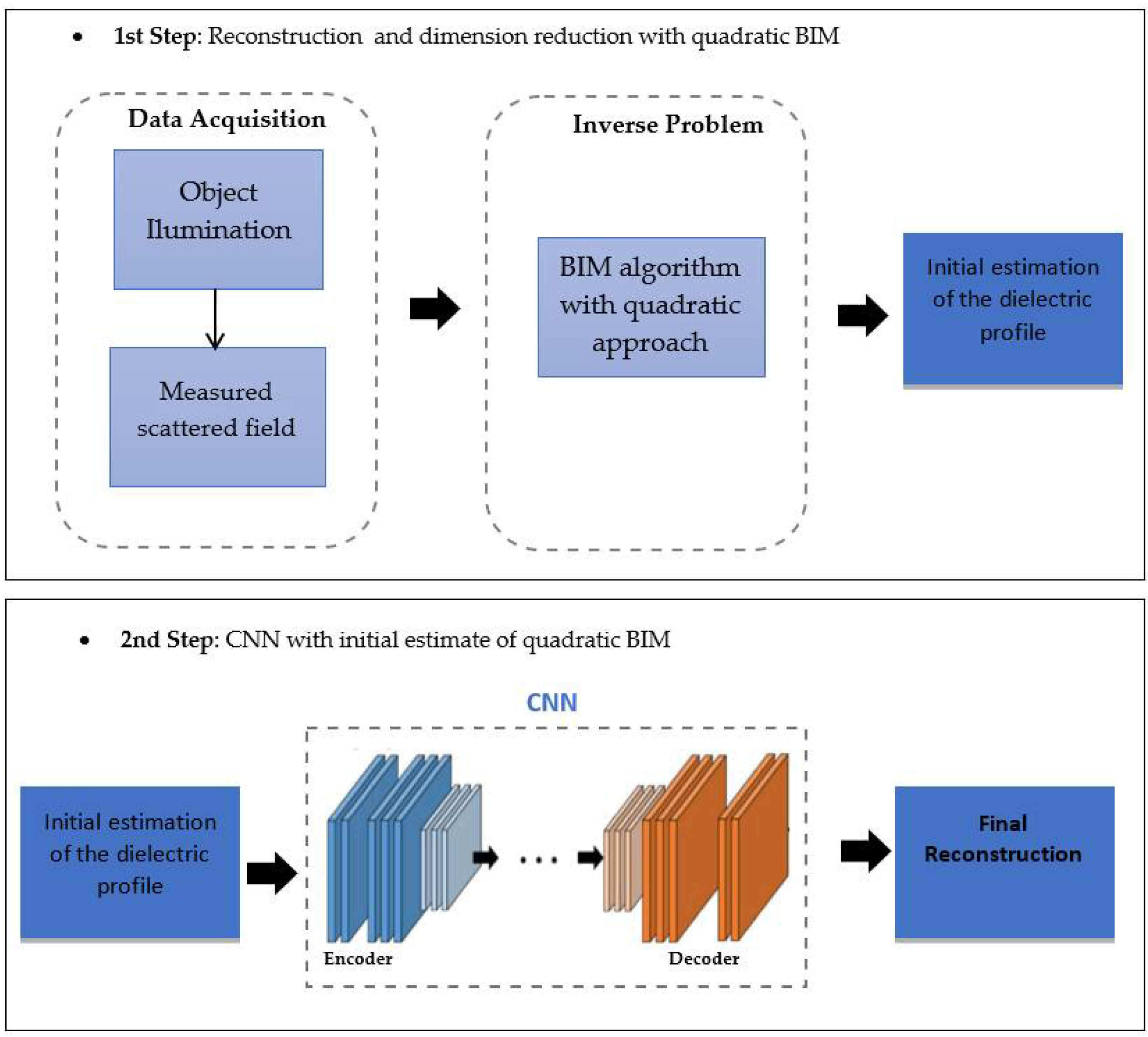
To solve the inverse scattering problem and retrieve an accurate dielectric profile after the BIM reconstruction, a machine learning methodology is employed (see Figure 2).

Indeed, the first step is to solve the inverse problem using the quadratic BIM, obtaining an initial estimate of the dielectric profile of the object under investigation. In particular, the initial and the reconstructed images are made up of 150 × 150 pixels and 64 × 64 pixels, respectively.

The second step is to resize the image produced by the BIM from 64 × 64 pixels to 128 × 128 pixels, which is then to be processed using the machine learning scheme. A particular CNN, which is based on the so-called U-net architecture [26], is adopted, as reported in Figure 3.

The U-Net architecture, initially used for image segmentation, can be considered as an encoder–decoder network. Specifically, looking at Figure 3, the left part of the network corresponds to the encoder and is responsible for reducing the spatial dimensions of each layer by increasing the channels. It consists of the repeated application of 3 × 3 convolutions, batch normalization, and a rectified linear unit (ReLU), followed by a 2 × 2 max pool resolution reduction which doubles the number of function channels with each step of resolution reduction. Instead, the right part of the architecture is given by the decoder, whose function it is to increase the spatial attenuations and reduce the number of channels. The decoder consists of a 3 × 3 up-convolution and two concatenations that are related to the trimmed feature maps of the encoder. Using this method, a prediction is made for each pixel of the input image.

The network training is carried out on a PC with CPU AMD Ryzen 7 5800 H, Radeon Graphics 3.20 GHz, and NVIDIA RTX 3060.

With the modification introduced in this paper, as described above, the reconstruction of each image by applying the BIM with a quadratic approach takes less than 5 min, thus considerably reducing the computational cost when compared to the previous work [21]. With the quadratic BIM, 500 images are generated; 95% are used for training and 5% are used for CNN validation. Moreover, 30 additional images are also generated for an unbiased evaluation of the final model. For the training of the network, a total of 13 h is required for 51 epochs, and subsequently it takes less than 5 s to perform the reconstruction of the dielectric profile when applying the trained CNN.

The training process can be sped up even further by employing more powerful GPUs or using parallel computation.

4. Numerical Results

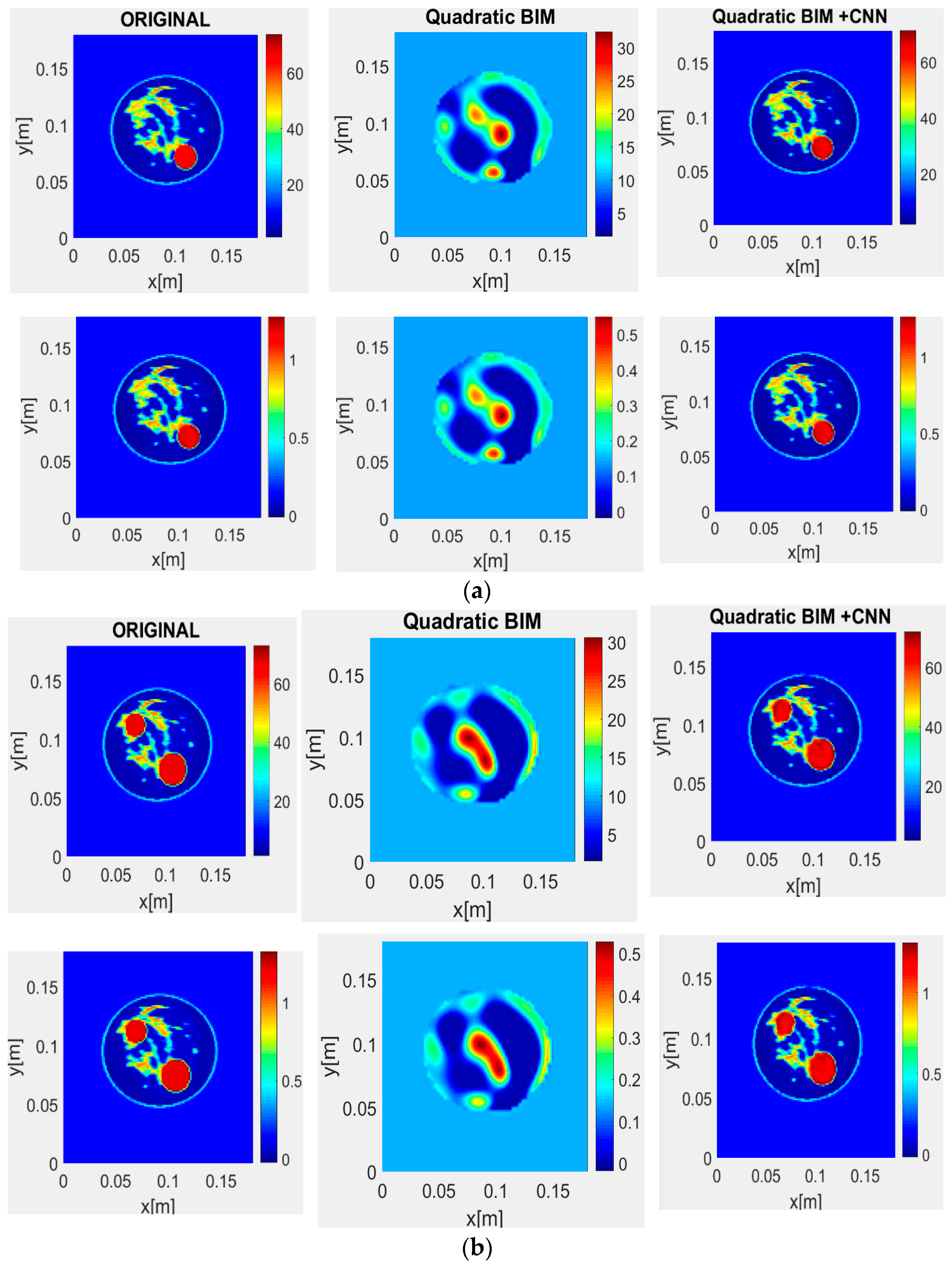
The proposed method is applied to a breast model obtained from the Numerical Breast Phantom Repository [28] of the University of Wisconsin Cross-Disciplinary Electromagnetics Laboratory (UWCEM). Specifically, the phantom used corresponds to: Class 3, Phantom 2, and Breast ID: 070604PA2. The dielectric profile of the adopted model is shown in Figure 4.

In the numerical tests, a domain of interest D with a size of 0.18 $\times$ 0.18 m or $\frac{3\mathsf{\lambda }}{5}\times \frac{3\mathsf{\lambda }}{5}$ is assumed, where λ is the free-space wavelength. There are 11 incident waves and 11 line receivers which are placed on a circle with a radius of 0.10 m, which includes the domain of investigation. A scattered field sampling is performed at an operating frequency of 1 GHz, taking into account that the best frequency to measure the relative permittivity and conductivity of malignant tumors is no higher than 1 GHz [7]. The values of permittivity range from 2.5 to 67 and take into account the minimum value of ${\epsilon }_{\mathit{r}}$ for the initial solution of the contrast map. On the other hand, a permittivity value of ${\epsilon }_b=10$ for the background is considered, especially when working with strong scatterers, to relax the maximum contrast of the dielectric constant [12].

The discretization is conducted at 150 × 150 pixels for the initial image and 64 $\times$ 64 pixels for the reconstructed image. The tests for the validation of the proposed scheme are performed for the breast phantom model, shown in Figure 2, by adding random tumors with diameters between 3 mm and 8 mm in various positions.

To perform a quantitative evaluation of the reconstruction performance of the proposed inverse scattering scheme, the following (percentage) relative error is considered:

$$R_e=\frac{1}{N_p} {\displaystyle \sum }_{n=1}^{N_p}\left[\frac{\left|{\epsilon }_{r\left(n\right)}^r-{\epsilon }_{r\left(n\right)}^t\right|}{{\epsilon }_{r\left(n\right)}^t}\times 100\%\right]$$

(9)

where:

–

${\epsilon }_{r\left(n\right)}^t$is the value of the true relative permittivity corresponding to the n-th pixel;

–

${\epsilon }_{r\left(n\right)}^r$is the value of the reconstructed relative permittivity corresponding to the n-th pixel;

–

$N_p$ is the total number of pixels.

In Figure 5, the variation in the relative error $R_e$ as a function of the number of training epochs, in training, validation, and testing, is reported. The behavior, denoted by a decreasing function, successfully demonstrates the effectiveness of the learning stage of the network.

The achieved result is optimal because the final relative error is small, the test and validation set errors have similar features, there is no major overfitting, and the best validation performance is achieved at epoch 51.

Figure 6 shows some representative tests obtained from the reconstruction procedure, where a comparison is made between the original model, the parameters reconstructed with the quadratic BIM, and those reconstructed in combination with the CNN. Comparisons are performed using data only from the test set, which is not considered during the CNN training. For all conducted tests, the use of CNN in the BIM with a quadratic programming approach produces a very noticeable improvement in the final reconstruction.

Predictions for the original breast model consisting of the reconstructed values yield a mean relative error value of 2.4104% and an accuracy of 97.5896%, for the group of 30 images taken of the test set. In particular, the accuracy is computed as $\left|100\%-R_e\right|$. The overall results are summarized in

Table 1. Sample statistics of the relative error (Equation (9)) to compare the BIM with the quadratic approach and the proposed model.

	Relative Error Quadratic BIM (%)	Relative Error Quadratic BIM+CNN (%)	Accuracy Quadratic BIM+CNN (%)
minimum	24.7	2	97
mean	27	2.4	97.6
median	26.9	2.4	97.6
maximum	30.7	3	98

. In particular, the first two columns report the relative error (minimum, mean, median, and maximum), as given by Equation (9), for the quadratic BIM and the quadratic BIM with CNN, respectively. In the third column, the accuracy is computed for the proposed BIM+CNN method, by considering that a minimum for the relative error corresponds to a maximum of accuracy.

To realize a comparison with the previously published results in [23], the same parameters reported in Table 1 are computed by applying the Frobenius norm and are summarized in

Table 2. Sample statistics of the relative error (Frobenius norm) to compare the BIM with quadratic approach and the proposed model.

	Relative Error Quadratic BIM [%]	Relative Error Quadratic BIM+CNN [%]	Accuracy Quadratic BIM+CNN [%]
minimum	63.4	4.6	91.2
mean	68.1	6.2	93.7
median	68.1	6	94
maximum	72	8.7	95.4

. Almost identical values are achieved for the accuracy when compared to those reported in [23], but with the advantage of a reduced number of training data (only 30 images), and the adoption of a single operating frequency (a multifrequency approach is applied in [23]).

5. Conclusions

In this paper, an improved machine learning-based methodology to solve inverse scattering problems has been investigated. In particular, it proved to be suitable in the case of highly nonlinear problems with strong scatterers. As a first step, the reconstruction process was performed using the BIM with a quadratic approach, obtaining the minimization of the inverse sub-problem and the knowledge of the upper and lower limits of the contrast values. Moreover, the use of a regularization procedure was shown to significantly improve the ability of this method to locate the profile of the strong scatterers. Subsequently, to improve the reconstruction, a CNN was applied, which allowed the microwave images to be reconstructed in a short time and with a high accuracy.

In comparison with the original method described in [23], the scattered field sampling was carried out only at a single frequency and the number of transmitting and receiving antennas was significantly reduced, thus leading to a considerable reduction in the computational cost. The obtained results clearly showed that the quadratic BIM approach in combination with the machine learning methodology greatly increased the accuracy of the reconstruction compared to using only quadratic BIM. The capacity and viability of the proposed method were demonstrated in terms of its resolution, accuracy, and speed of convergence in high-contrast objects, such as breast tissue. It obtained an average error of 2.4% and an accuracy greater than 96% for all the performed tests, despite having a single operating frequency and a reduced number of training data.

Future research is needed to involve the adoption of the proposed approach to build 3D models of human tissues, exploiting the potentialities that are being developed at the ERMIAS Laboratory of the University of Calabria in the realization of suitable phantoms with characteristics similar to human tissues [29].