Prediction of Power Output from a Crystalline Silicon Photovoltaic Module with Repaired Cell-in-Hotspots

Abstract

Recycling of problematic photovoltaic modules as raw materials requires considerable energy. The technology to restore cells in hotspot modules at a relatively low cost is more economical than replacing them with new modules. Moreover, a technology that restores power by replacing a cell-in-hotspot of a photovoltaic module with a new cell rather than replacing the whole module is useful for operating power plants. In particular, power plants that receive government subsidies have to use certified modules of specific models; the modules cannot be replaced with other modules. Before putting resources into module restoration, predicting the power of a module to be restored by replacing a cracked cell with a new cell is essential. Therefore, in this study, the module output amount after restoration was calculated using the previously proposed relative power loss analysis method and the recently proposed cell-to-module factor analysis method. In addition, the long-term degradation coefficient of the initial cell and the loss due to the electrical mismatch between the initial and new cell were considered. The output of the initial cell was estimated by inversely calculating the cell-to-module factor. The differences between the power prediction value and the actual experimental result were 1.12% and 3.20% for samples 190 A and 190 B, respectively. When the initial rating power and tolerance of the module were corrected, the differences decreased to 0.10% and 2.01%, respectively. The positive mismatch, which restores cells with a higher power, has no loss due to the reverse current; thus, the efficiency of the modules is proportional to the average efficiency of each cell. In this experiment, the electrical mismatches were only 0.37% and 0.34%. This study confirmed that even if a replacement cell has a higher power (<20%) than the existing cell, the power loss is not significantly affected, and heat generation of the existing normal cell is not observed. Hence, it was concluded that when some cells are damaged in a crystalline solar cell, the module could be restored by replacing only those cells instead of disposing of the entire module. However, for commercialization of the proposed method, a long-term reliability test of the module repaired using this method must be performed to confirm the results. Following this, recycling cells instead of recycling modules will be an economical and eco-friendly alternative.

1. Introduction

Renewable energy, including photovoltaic power generation, has steadily increased globally through [1,2] continuous cost-cutting efforts based on eco-friendly elements and low maintenance costs [3,4], despite the high costs and relatively low economy in the early stages of its implementation [5]. Owing to economic security and increased supply of renewable energy [6,7], the achievement of grid parity has recently accelerated [8,9], with a certain percentage of fossil fuel usage steadily being replaced by renewable energy usage, and hence, the total use of renewable energy has increased over the past decade [10]. Expanding the solar energy supply may reduce carbon dioxide emissions and achieve a healthy mix of energy sources to overcome the climate crisis [11,12]. However, the increasing demand for solar energy may cause shortages of the resources used in the advanced production of solar modules [13,14,15]. In particular, owing to the scarcity of resources such as silver, indium, and bismuth, target material consumptions of 2, 0.38, and 1.8 mg/Wp [16,17], respectively, have been proposed; thus, a significant reduction in material consumption is required to expand renewable energy supply [18].

The large-scale installation of photovoltaic modules results in the problems of economic use of resources during production and processing of waste modules after use [19,20]. By 2050, 80 million tons of accumulated photovoltaic modules are expected to reach their service life worldwide, with 10 million tons in the US alone [21]. With the rapid increase in the installation of photovoltaic modules in countries such as China, the collection and recycling of end-of-life photovoltaic modules is becoming an important task, and various methods of building efficient recycling systems are being investigated [22]. According to previous studies, the predicted accumulated waste that will be generated from 2020 to 2080 in existing solar power plants varies in proportion to solar installations, and is expected to peak at 130,000 tons in 2051 and 141,297 tons in 2054 [23]. Currently, the life of a photovoltaic module is approximately 20–30 years; therefore, the life of photovoltaic modules installed in the early 2000s will expire on a large scale, and the disposal of waste modules will increase rapidly. Photovoltaic modules consist of expensive materials, such as aluminum, silver, copper, tin, and silicon wafers. In addition, they can be used as highly attractive recycled materials in terms of the environmental charges imposed when filling landfills. In the recycling process of a general photovoltaic module, research has primarily focused on recycling by collecting silicon wafers and refabricating them into optimized silicon solar cells [24,25], pyrolyzing organic materials such as ethylene vinyl acetate (EVA) [26], and removing organic materials such as glass and ribbon metals [27,28]. As a research example on recovering the performance of photovoltaic modules, a technology for recovering the insulation resistance of aging modules by injecting coatings based on polyurethane, epoxy, silicone, and synthetic rubber of crystalline photovoltaic modules was introduced [29,30]. However, recycling or reuse technology generally involves removal of frames, junction boxes, or cables, etc., from crystalline photovoltaic modules, followed by thermal or chemical decomposition of the laminated module to collect glass, silicon, metal, and polymer [31,32].

This recycling technology is not currently widely used because it is expensive and the return on investment (ROI) is less than approximately −0.25 as of 2022 [33]. In addition, the recycling method, which involves collecting the raw materials separately, is not applicable to the recovery of damaged modules in an operating power plant because the failure of a part of the module results in the crushing of other usable parts. Accordingly, this paper proposes a technology to recover photovoltaic modules at the same or a higher level of the initial power value by replacing cells at a safety risk, such as power loss and hotspots, owing to damage to some cells of an aged silicon photovoltaic module. Most commercial solar power plants receive subsidies from the government. In this case, only certified modules of a particular model should be used during the generation period. If the module fails, it cannot be replaced by another model. Moreover, owing to the rapid improvement in cell efficiency every year [34,35], the module model continues to change. In commercial power plants, restoring the output of a module by cell replacement is very useful. Technological advancements in the restoration of the module result in a power deviation between the initial and new cell [36,37]. Therefore, when replacing a cell with a new cell having a higher power, the possibility of an electrical mismatch loss occurring should be considered, and the long-term power degradation of the initial cell should be confirmed. Hence, the purpose of the experiment was to determine the extent to which the output improvement of the new cell is reflected in the output of the module to be restored. Previous studies have shown that the prediction of power mainly includes power degradation in modules with hotspots or how much power decreases as a result of EL in modules with potential-induced degradation (PID) [38,39]. However, the purpose of this study was to predict the improvement to power through replacement of damaged cells in a module, which has not been attempted before. The results of this study suggest that the energy and environmental costs of recycling modules can be significantly reduced by reusing waste modules in more diverse states.

2. Experiments

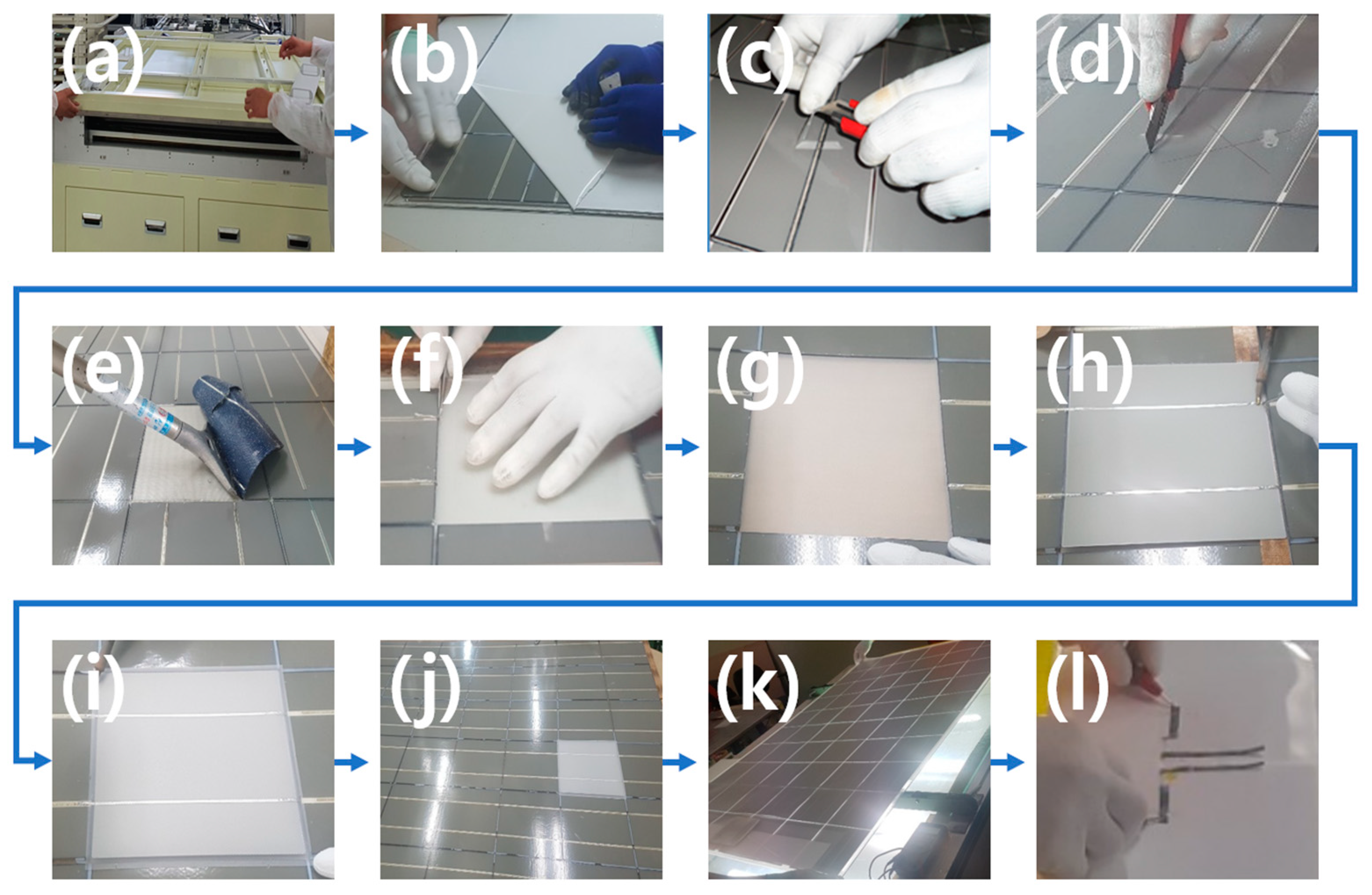
2.1. Methods and Procedures

The overall experiment was conducted in the following order: module power output and defect verification, calculation of grade of originally applied cells, grade verification of replacement cells, power prediction, module power recovery, comparison of predicted power output and experimental results, and application of correction values. First, the defects and power output of the module to be recovered were checked via electroluminescence (EL) measurement and a sun-simulator. EL measurements are used to identify internal defects that cannot be visually identified using EL in solar cells.

Table 1. Nomenclature for the electrical characteristics of the module.

Isc	Short-circuit current	Imp	Current at the maximum power output
Voc	Open-circuit voltage	Vmp	Voltage at the maximum power output
Pmax	Maximum power output	FF	Filling coefficient factor

provides the nomenclature for the electrical characteristics of the module.

The current corresponding to the cell I_sc and the voltage at the same level as the module V_oc were applied for the measurement. EL images of the module were captured in several parts of a darkroom, recollected, and displayed on a screen. The EL equipment manufactured by MC Science in Korea was used for the measurements. The simulator measures the module’s I_sc, V_oc, P_max, etc., under the standard test condition (STC) at 25 °C, 1 Sun (1000 W/m²), and air mass 1.5, and corrects the actual temperature to output the calculated value to the screen. The equipment used in this study was a Spire-Nissinbo Sun Simulator. The equipment was calibrated for proper use in the certification test of the photovoltaic module by receiving the AAA in three evaluation items: uniformity, stability, and spectrum. Measurements of power output from equipment are displayed in various ways, i.e., 1–4 digits after the decimal point; however, in this study, the third digit after the decimal point was rounded to two digits to maintain consistency. The CTM (cell to module) factor calculation method was applied to the power analysis of the cells used at the time of manufacturing the target samples and the review of the cells to be replaced [40]. The grade of the applied cell was inversely calculated based on the initial power output of the module disclosed on the Internet by the manufacturer. The module power after cell replacement was predicted after checking the grade of the cell to be replaced.

The CTM coefficient k-factor calculation method was used to analyze the power of the original cell of the target samples and review the replacement cell. Manufacturing modules from cells, models, and formulas for classifying the CTM coefficient k-factor, which affects efficiency or power, and analyzing loss or acquisition mechanisms have been presented in previous research [41,42]. If the dimension data and rated power of a module released by the module manufacturer are the initial power outputs of the module, the module efficiency is calculated to be 13.6%. Because the module power output is calculated from the sum of the CTM coefficient k factor and the initial solar cell power in the module power output calculation model, the power output of the module can be calculated using Equations (1) and (2) [41,43]. The factors i and m in Equations (1) and (2) are variables of the routinely used pie function, and refer to the extension of the CTM factor. The CTM k-factor consisted of 15 types: k₁ (module margin), k₂ (cell spacing), k₃ (cover reflection), k₄ (cover absorption), k₅ (cover/encapsulant reflection), k₆ (encapsulant absorption), k₇ (interconnection shading), k₈ (cell/encapsulant coupling), k₉ (finger coupling), k₁₀ (interconnector coupling), k₁₁ (cover coupling), k₁₂ (cell interconnection), k₁₃ (string interconnection), k₁₄ (electrical mismatch), and k₁₅ (junction box and cabling). The meaning of I = 3−m in the ∏-function of Equation (1) means CTM k-factor from k₃ to k₁₅. Then, the sum of the cell power outputs from j = 1−n from the ∑-function is the number n of cells applied to the module.

$${\mathit{P}}_{\mathit{m}\mathit{o}\mathit{d}\mathit{u}\mathit{l}\mathit{e}}={\displaystyle \mathbf{\prod }}_{\mathit{i}\mathbf{=}\mathbf{3}}^{\mathit{m}}{\mathit{k}}_{\mathit{i}}\mathbf{·}{\displaystyle \mathbf{\sum }}_{\mathit{i}\mathbf{=}\mathbf{1}}^{\mathit{n}}{\mathit{P}}_{\mathit{c}\mathit{e}\mathit{l}\mathit{l}\mathbf{.}\mathit{j}}$$

(1)

$$\mathit{C}\mathit{T}{\mathit{M}}_{\mathit{p}\mathit{o}\mathit{w}\mathit{e}\mathit{r}}\mathbf{=}{\displaystyle \mathbf{\prod }}_{\mathit{i}\mathbf{=}\mathit{3}}^{\mathit{m}}{\mathit{k}}_{\mathit{i}}$$

(2)

In terms of module efficiency, factors affecting the entire area of a gap module between modules are important; however, when a module is produced from a cell, a design margin (k₁) to ensure an electrical insulation distance and a loss factor (k₂) owing to the cell interval are not related to a power change. The module efficiency can be expressed by Equations (3) and (4) [41].

$${\eta }_{module}=\frac{P_{module}}{E_{STC}·(A_{module}+A_{cell spacing}+A_{cells)}}$$

(3)

$${\eta }_{module}=\overline{{\eta }_c}·\left(k_1+k_2-1\right)·{\displaystyle \prod }_{i=3}^m{k}_i$$

(4)

Therefore, according to this model, the module efficiency is proportional to the average efficiency of the cell rather than being dominantly affected by the lowest efficiency. The average efficiency of the cell was calculated by considering the electrical mismatch loss (k₁₄) of the cell to predict the power output of the module to be restored. For the loss caused by the electrical mismatch of cells, studies were published prior to research on the CTM factor, and the widely known definition of RPL is expressed as the difference between the maximum power (P_mpc) of n individual cells connected in series to form a cell string or module. RPL can be expressed as Equation (5) from the difference between the sum of the maximum power of all cells and the maximum power of the module.

$$RPL=\frac{{{\displaystyle \sum }}_{i=1}^n·P_{mpci}-P_{module}}{{{\displaystyle \sum }}_{i=1}^n·P_{mpci}}$$

(5)

In theory, when individual cells operate completely independently, the maximum power output is denoted as P’_max, and when the average cell power output value in a group is P_max, the calculation of RPL_B (relative power loss of a module using Bucciarelli’s equation) is as shown in Equation (6).

$$RP{L}_B=\frac{P_{max}^{\prime }-P_{module}}{n·I_{mp}^{-}{V}_{mp}^{-}}$$

(6)

The power output after cell replacement and the state inside the module were also confirmed using the EL and Sun simulators. The cell replacement process is discussed in the next section. After cell replacement, the gain factor (power increment of the replacement cell), loss factor (long-term degradation, electrical mismatch), and unidentified tolerance parts of the module track the experimental results and apply the same to the two samples, correct the power predictions, and finally compare them with the results.

2.2. Experiments

Figure 1 presents an EL image of a 6-inch 54-cell 3BB polycrystalline silicon solar module, where the hose power degrades owing to cell damage. Figure 1a shows the first sample of 190-Wp grade, referred to as 190 A for convenience, and its appearance. Figure 1b–d depict EL images of 190 A, the second sample of the 190-Wp class (190 B), and 190 B, respectively. As shown in images (a) and (c), a weak yellowish appearance, which was not severe, was observed. In addition, approximately six to nine dark areas were observed in the EL image (Figure 1b) and approximately six dark areas were observed at 190 B (Figure 1d). In the green-marked cell of (d), the dark area in the cell occurred because of poor soldering between the mutual connector and the busbar.

The modules used in this study included samples collected from commercially operated power plants; however, the current–voltage (I–V) data at the time of manufacture were unknown. Therefore, the electrical characteristics of the model disclosed by the manufacturer were assumed as the initial electrical performance.

Table 2. Electrical data of the modules in the initial stage and after use.

Sample			Pmax (Wp)	Isc (A)	Voc (V)	Imp (A)	Vmp (V)	FF	Tolerance
190 A	54 cells	initial	190.00	7.89	33.00	7.31	26.00	0.73	±3%
		failed	148.80	8.16	32.77	5.16	28.84	0.56
190 B	54 cells	initial	190.00	7.89	33.00	7.31	26.00	0.73	±3%
		failed	139.70	7.95	32.67	5.67	24.66	0.54

lists the initial electrical specifications of samples 190 A and 190 B and the electrical data of the failed samples after a certain period of operation. As confirmed in the EL image, the FF was severely degraded by the damaged cells in the middle of the string. For 190 A and 190 B, the power decreased by −21.69% and −26.47%, respectively.

Figure 2 displays the I–V and voltage–power (V–P) curves of modules 190 A and 190 B. The I–V curves appear step-shaped, while the V–P curves have two or more multi-peaks, which is a typical form caused by the decrease in Isc due to the cracking of a specific cell in a cell string [44].

Figure 3 shows the process of removing the broken cells of 190 A and 190 B cells and replacing them with new cells. (a) First, the module is placed on a hot plate to heat the sun-side and soften the EVA, then, the back sheet is removed from the edge. (b) When the back sheet is completely peeled off, (c) the tape attached to fix the cell-string gap was removed. If it is a material such as EVA, it does not require removal; however, for a tape using polyethylene terephthalate (PET) as a basic material, a gap is formed between the tape and cell owing to the loss of adhesion.

When cleaning the back sheet removal surface or the cell removal area using ethanol or isopropyl alcohol (IPA), the permeated organic solvent may cause solvothermal swelling in the lamination process, or gas may accumulate to cause swelling [32].

3. Result and Discussion

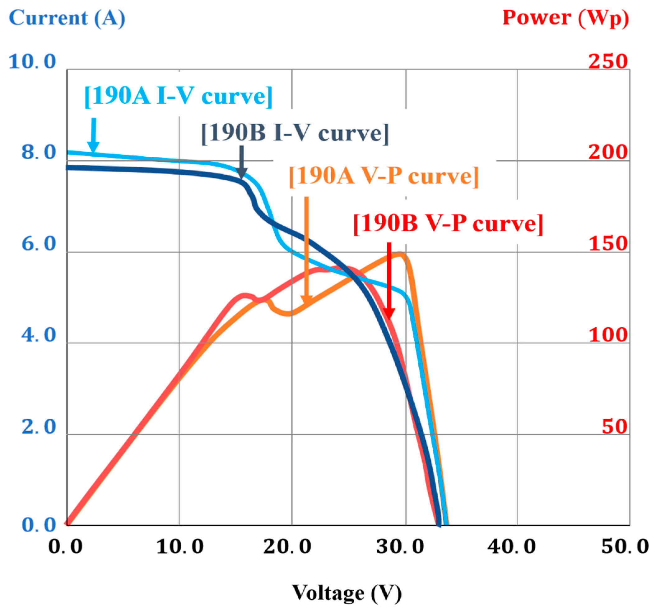
3.1. Power Output Analysis of Initial Cells Applied to Each Sample and Specification of Replacement Cells

The initial CTM of the cells analyzed above was approximately 1.78% based on power, with the median value of 0.9%, as suggested in the optimized module process published in a previous study, and 2.72% of the CTM value of a general photovoltaic module [41]. The calculated power output of the individual cells was approximately 3.6 Wp, which is approximately 14.8% in terms of cell efficiency.

Table 3. Initial applied cell grade analysis of sample modules (190 A, 190 B) to be recovered.

CTM Factor (k)	K conventional (%)	CTM power Ratio	Initial CTM power of 190 A, 190 B
Module efficiency (STC)/Power	18.31	98.23%	190.0
k15 (junction box and cabling)	−0.05	−0.23%	−0.45
k14 (electrical mismatch)	−0.04	−0.19%	−0.36
k13 (string interconnection)	−0.03	−0.14%	−0.27
k12 (cell interconnection)	−0.037	−0.17%	−0.33
k11 (cover coupling)	0.28	1.30%	2.51
k10 (interconnector coupling)	0.09	0.42%	0.81
k9 (finger coupling)	0.17	0.79%	1.52
k8 (cell/encapsulant coupling)	0.16	0.74%	1.43
k7 (interconnection shading)	−0.44	−2.04%	−3.94
k6 (encapsulant absorption)	−0.03	−0.14%	−0.27
k5 (cover/encapsulant reflection)	−0.01	−0.02%	−0.05
k4 (cover absorption)	−0.14	−0.65%	−1.26
k3 (cover reflection)	−0.31	−1.44%	−2.78
Cell efficiency (STC)/Power	21.58	100.00%	193.45

lists the initial power output of the cell applied to the module using Equations (1) and (2).

As cells of the same grade were already discontinued, a module was repaired using the 3-bus bar cell, which had the lowest power among the cells currently in use. The P_max and cell efficiency of the cell used in the initial manufacture of the module are listed in Table 2. Assuming that the FFs of the module and cell were the same, the cell V_mp and V_oc were calculated by considering the number of cells from the module V_mp and V_oc, and I_sc and I_mp were determined using P_max and FF of the cell.

The electrical characteristics of the initial and replacement cells used to restore the modules are presented in

Table 4. Electrical data of initial cell and replacement cell.

Item	Eff. Cell	Pmax (Wp)	Isc (A)	Voc (V)	Imp (A)	Vmp (V)	FF	Tolerance
Initial cell	14.80	3.58	8.07	0.61	7.32	0.49	0.73	±3%
Replacement cell	17.60	4.28	8.62	0.63	8.39	0.51	0.78	±3%

. The tolerance of the initial cell follows that of the module specification sheet.

3.2. Predicting the Power Output of the Restore Module When Applying A Replacement Cell

The following are the considerations for predicting the power of a module to be recovered when a new cell is installed: the first element is the deviation between the actual power output of the initial module and rated power output. This part was expected to be within the initial tolerance range, and after module recovery, the results and discussion were verified. Next, the power increase of the replacement cell should be added and the value of the field-aged power degradation rate from the initial power of the existing cell should be deducted. Moreover, the loss from the electrical mismatch between the cells should also be considered. The increase in the power of the replacement cell can be easily calculated using Equations (2) and (4). The next part to be considered is the loss caused by the electrical mismatch. A recent study reported that the result of power loss from the electrical mismatch of cells within a module was difficult to determine; however, when the direct parallel configuration of modules was different, the relative power loss (RPL) of the array due to electrical mismatch was 1.3–2.6% [45]. In previous studies, the power loss caused by the electrical mismatch of cells was reported to be approximately 0.009–0.19% [46]; thus, it is already reflected as −0.19% in the CTM factor; therefore, it should be applied conservatively. In the prediction of the power output, the final part to be considered is the loss from power degradation owing to the field aging factor of the existing cell. In general, the rate of power output degradation guaranteed by a module manufacturer is 0.7%/year, which is a guaranteed limit design considering the power degradation caused by the failure of some modules in PV power plants. Referring to the results reported in a previous study, the actual power output degradation rate of more than 80% for crystalline PV modules in PV power plants that have been operated for more than 10 years is approximately 0.27%/year on average [47]. This figure is significantly lower than the limit guaranteed by manufacturers. In this study, we applied this figure to calculate the power output prediction.

Table 5. Power output prediction for recovered modules.

CTM Factor (k)	CTM Power Ratio	190 A (10 New Cells)	190 B (6 New Cells)
Module efficiency (STC)/Power	98.23%	196.40	193.50
Long term degradation of used cell	−0.27% × (% of remaining cell)	−0.34(−0.17%)	−0.47(−0.24%)
k15 (junction box and cabling)	−0.23%	−0.46	−0.46
k14 (electrical mismatch)	−0.19%	−0.37	−0.37
k13 (string interconnection)	−0.14%	−0.28	−0.28
k12 (cell interconnection)	−0.17%	−0.34	−0.34
k11 (cover coupling)	1.30%	2.60	2.56
k10 (interconnector coupling)	0.42%	0.84	0.82
k9 (finger coupling)	0.79%	1.58	1.56
k8 (cell/encapsulant coupling)	0.74%	1.49	1.46
k7 (interconnection shading)	−2.04%	−4.08	−4.03
k6 (encapsulant absorption)	−0.14%	−0.28	−0.28
k5 (cover/encapsulant reflection)	−0.02%	−0.05	−0.05
k4 (cover absorption)	−0.65%	−1.30	−1.28
k3 (cover reflection)	−1.44%	−2.88	−2.84
Cell power (STC, + power gain)	100.00%	200.32	197.52

lists the power output predictions for the recovered modules.

For 190 A, 10 broken cells were replaced; thus, (10 × 4.28 Wp) + (44 × 3.58 Wp) = 42.8 + 157.52 = 200.32 Wp is the total power output value of the cell. In 190 B, six cells were replaced: (6 × 4.28 Wp) + (48 × 3.58 Wp) = 25.68 + 171.84 = 197.52 Wp. The results are presented in Table 4. Through the calculation, the predicted power output values of 190 A and 190 B were calculated as 196.40 Wp and 193.50 Wp, respectively. The CTM factor k_i values ranging from k₁ to k₁₅, and k₃ to k₁₅ are shown in the table; however, k₁ and k₂ values are not shown in the table nor described here. The CTM factor k₁ is the module margin, which is approximately −2.03% in a typical module, and k₂ is the cell spacing, which is also generally −0.53%. This value is a design factor for the module area and depends on module dimensions. However, the module margin or cell interval for insulation distance affects only the area efficiency of the module and does not produce power by itself; therefore, the calculation of CTM power was excluded from previous research.

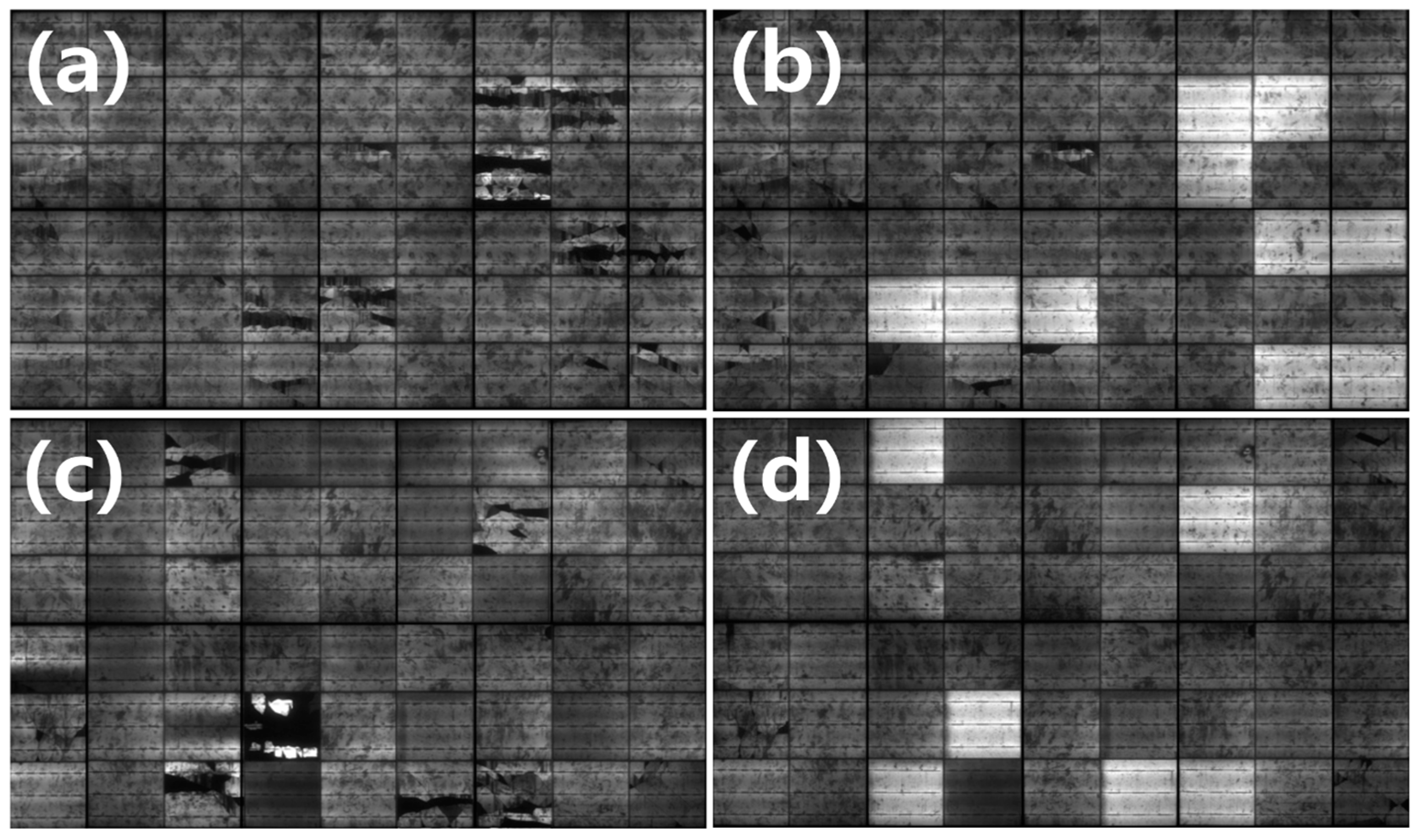
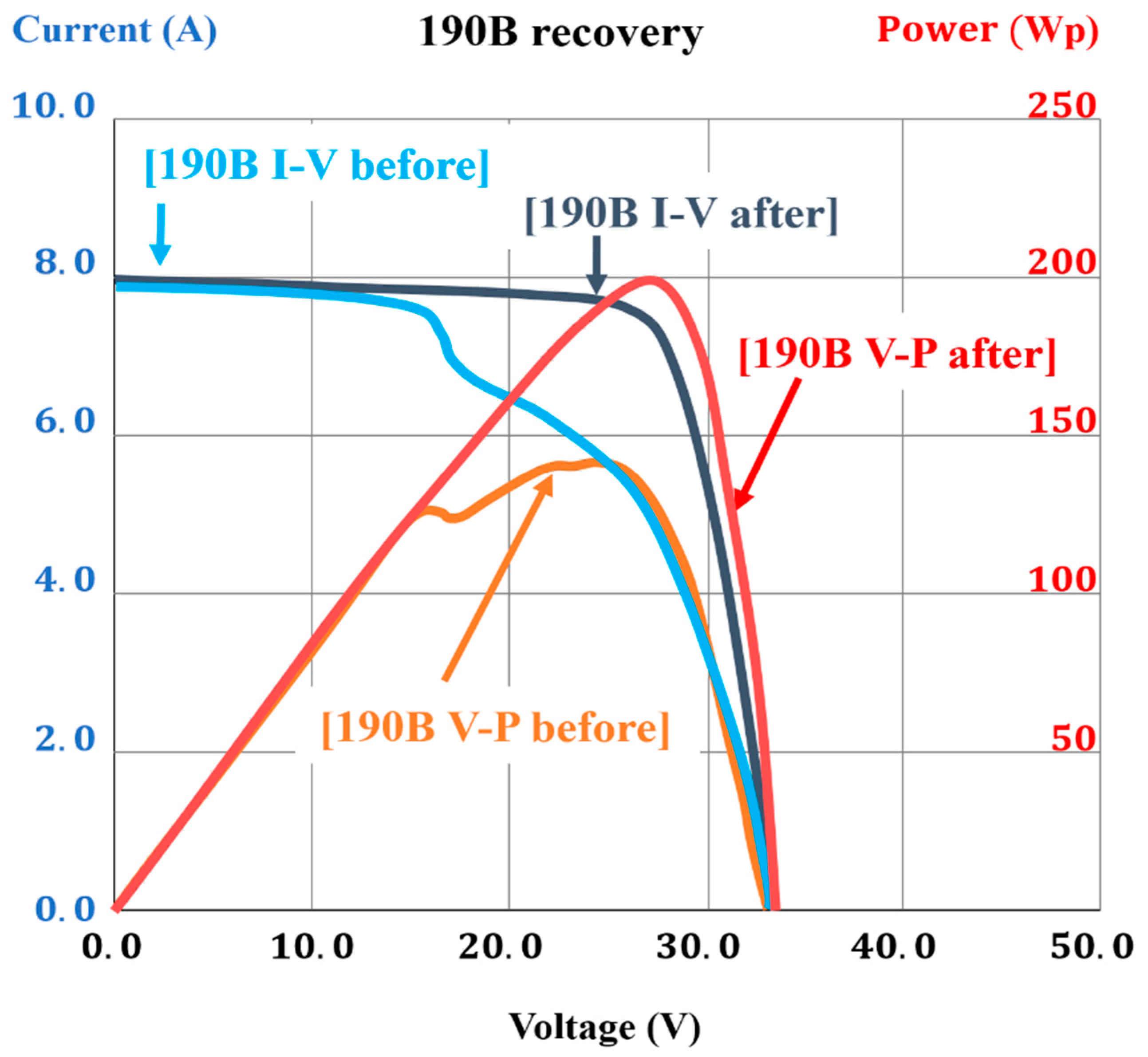
3.3. Results of Power Recovery by Cell Replacement of 190 A and 190 B Samples

Figure 4 shows a comparison of the EL images of the modules before and after repair.

In Figure 4c,d, the relatively bright cells are the newly replaced cells. In Figure 4a, when replacing cells of the 190 A sample, one more cell was replaced by damaging adjacent cells while removing the cells from the hot plate, and as the cell replacement operation was repeated, the same mistake was not repeated. Some small cracks not shown in Figure 4a are observed in Figure 4b, which are defects occurring during manual cell removal. However, the result shown in Figure 4d is not much different from that in Figure 4c because cell replacement has become familiar and cell removal progressed much more easily. For an easy recovery process, care should be taken to prevent additional cell cracks when collecting and reinstalling the modules to be repaired.

Table 6. Electrical data of modules before and after recovery.

Item	Replacement		Pmax (Wp)	Isc (A)	Voc (V)	Imp (A)	Vmp (V)	FF	Initial Comparison
190 A	10 cells	before	148.80	8.16	32.77	5.16	28.84	0.56	−21.69%
		recovery	198.60	8.11	32.95	7.54	26.35	0.74	+4.53%
190 B	6 cells	before	139.70	7.95	32.67	5.67	24.67	0.54	−26.47%
		recovery	199.70	7.99	32.89	7.50	26.64	0.76	+5.11%

lists the electrical characteristics of the module before and after recovery. The module power increased by approximately 4.50% to 198.60 Wp from the rated power for 190 A, and by approximately 5.10% to 199.70 Wp for 190 B. We verified that, considering the loss of electrical mismatch between the existing cell and the new cell, the higher power of individual cells had a greater effect on the power of the module.

As mentioned in Section 3.2, when the difference in cell mismatch is not large, the loss due to mismatch is insignificant in the range 0.10–0.19%, and most (>80%) of crystalline photovoltaic modules are only approximately 0.27%/year on average. Therefore, it matches well with the result that predicted that the gain factor would have a greater impact on the final power output of the module than the loss factor [46,47].

Figure 5 and Figure 6 show the I–V curves before and after power recovery for 190 A and 190 B, respectively. The results in Figure 5 and Figure 6 show that I_sc and V_oc do not change significantly before and after module restoration and that the V–P curve is deformed by cell breakage, the FF is recovered, and the power of the module is restored.

As shown in Figure 5 and Figure 6, both the cell-in-hotspot-specific stepped I–V and multipeak-shaped V–P curves are recovered.

Figure 7 and Figure 8 show a brief circuit diagram of module 190 A before and after recovery, respectively. In the figures, I_ph represents the solar irradiance and I_pv represents the power output current. D₁, D₂, and D₃ denote bypass diodes #1–#3, respectively, and R_s denotes the series resistance.

In the EL image of Figure 7, nine cells were cracked, resulting in resistance loss. In this case, the ratio of shaded (or inactive) areas causing hot spots in the cell increased proportionally with the range of inactive areas between 20% and 50%. If the resistance becomes excessively large over a greater range or if the bypass diode is short-circuited [48], it causes 100% power loss to the entire connected string [49,50]. A part looks relatively brighter around the interconnector immediately next to the dark area of the damaged cell, and the current is concentrated on a part of a cell with relatively low resistance owing to cracks; thus, power loss occurs in the shaded and connected cells.

Figure 8 shows the EL of the module whose power was recovered after the cell replacement of the 190 A sample and its diagram. The picture for 190 B is repeated, so I omit it.

3.4. Comparative Analysis of Power Recovery Results and Predicted Values

Table 7. Comparison of predicted and experimental values.

Item	Before Recovery	Predicted Value	Experimental Value	Difference	Tolerance
190 A	148.80	196.40	198.60	+1.12%	±3%
190 B	139.70	193.50	199.70	+3.20%	±3%

shows the difference between the predicted power output value obtained using the CTM analysis before module recovery and the value measured after cell replacement.

Even when applying the power deviation when manufacturing a module, both cases exhibited a positive deviation; therefore, the loss, such as electrical mismatch, in the CTM factor was considered conservative among the possible ranges. The CTM power analysis results at 190 A are shown in Figure 9.

The sum of the power of the initial and replacement cells was defined as 200.32 Wp using the values calculated in Equation (1) and Table 4, and when CTM factors were applied, the predicted value of 198.60 Wp was determined. Here, if 2.20 Wp, i.e., the difference from the experimental results, was reflected, it was analyzed, as shown in Figure 9. The difference between the predicted and experimental result for 190 A was 1.12%, which fell within 3% of the power output tolerance value of the initial module. The analysis result of sample 190 B indicated that the error was larger. Figure 10 shows the CTM power analysis of the recovered module (190 B).

Sample 190 B was of the same grade as 190 A, and because there were fewer replacement cells (six), the power acquisition from the replacement cell was smaller than that at 190 A; therefore, the total power output of the cell was calculated as 197.52 Wp. In addition, the numbers of remaining cells in 190 A and 190 B were 44 and 48 cells, respectively; thus, the long-term degradation was then calculated to be −0.47 Wp, which is greater than −0.34 Wp for 190 A. The experimental value was 199.70 Wp, i.e., 6.20 Wp higher than the predicted value of 193.50 Wp. This is approximately 3.20% higher than the predicted value of 3% or more, which is the power output tolerance value of the initial module.

3.5. Analysis of Prediction Error and Correction of Prediction Value Reflecting Initial Tolerance

The error begins with the sum of the cell power output values. The final power value was 199.70 Wp, and the sum of the calculated cell power values was 197.52 Wp, which began with a difference of 2.18 Wp even if the CTM was assumed to be “0.” The value 2.18 Wp was 1.15% of the initial rated power value of 190 Wp, which was within the allowable tolerance range of the module. Therefore, assuming that the initial use cells of 190 A and 190 B were the same, sample 190 B corrected the experimental deviation of 2.18 Wp. Those of 190 A were calculated by adjusting the number of cells to calculate the correction value of 2.00 Wp. Accordingly, the predicted power output values of 190 A and 190 B could be recalculated as listed in

Table 8. Analysis of predicted and experimental values.

Item	Predicted Value	Tolerance Calibration	Correction	Experimental Value	Difference
190 A	196.40	2.00	198.40	198.60	+0.10%
190 B	193.50	2.18	195.68	199.70	+2.01%

. The initial power output prediction value of sample 190 A was 196.4 Wp. For the power correction value of 1.998 Wp within the tolerance shown in the experimental result, the correction prediction value was 198.4 Wp. Additionally, the error decreased to 0.10% with the final experiment result of 198.6 Wp. When the initial power output prediction value of 193.5 Wp was corrected for 190 B, the corrected prediction value was 195.68 Wp, which was approximately 2.13% lower than the experimental result for 199.7 Wp.

When the tolerance value calculated above was added to the initial rated power, the initial power of the module was approximately 192.45 Wp. Based on this, the power before and after module recovery owing to cell damage and the recovery trend of the FF are shown in Figure 11.

Table 9. Electrical data deviation of initial, faulty, and recovered module.

Item			Pmax (Wp)	Isc (A)	Voc (V)	Imp (A)	Vmp (V)	FF	Tolerance
	54 cells	initial	190.00	7.89	33.00	7.31	26.00	0.73	±3%
190 A		failed	148.80	8.16	32.77	5.16	28.84	0.56	−
		recovered	198.60	8.11	32.95	7.54	26.35	0.74
	Rate of decline (initial)		+4.53%	+3.55%	−0.16%	+3.13%	+1.36%	+1.92%
190 B		failed	139.70	7.95	32.67	5.67	24.67	0.54	−
		recovered	199.70	7.99	32.89	7.50	26.64	0.76	−
	Rate of decline (initial)		+5.11%	+1.28%	−0.33%	+2.57%	+2.42%	+4.11%

summarizes the initial, failed (before recovery), and recovered (after recovery) values of the power degradation module owing to cell cracking.

The characteristic of the recovery of the cell in the hotspot module by cell replacement is that the V_oc value hardly changes step-by-step but decreases within the error range by step. The largest negative mismatch factor in the phase of the power drop to the cell in the hotspot was I_mp, exhibiting a 29.43% decrease at 190 A compared with the initial value, which had the greatest impact on the power decrease of −21.69%. Even in sample 190 B, I_mp degradation caused a −22.48% decrease in the cell in the hot spot stage, and a power degradation of −26.47% was also the largest factor. For a positive mismatch with a high power, the I_sc and I_mp values both increased, and the V_mp value decreased step-by-step at 190 A; thus, the factor that most affected the positive mismatch was the increase in I_sc and I_mp; the increase in I_mp, in particular, was the largest factor. Figure 12 shows the EL images of samples (a) 190 A and (b) 190 B recovered by cell replacement, and (c) IR images measuring whether the module generated heat by installing them again in the power plant.

A difference in brightness was observed between the replaced and existing cells in the EL images shown in Figure 12a,b, but in Figure 12c, no significant heat generation was observed in the IR image at the installation site. The IR camera used to measure cell heat generation was a Ti400 FLUKE equipment.

Thus, we confirmed the restoration potential of modules that are underpowered by cells in hotspots in commercial power plants. When some cells are damaged in a crystalline PV module, the module can be restored by replacing those cells instead of discarding the entire module. Assuming that this method restores more than 180 sheets per day on a 200-Wp module basis, the cost of restoring the module is approximately 0.17 $/Wp. This is slightly more than half of the recent crystalline module price of 0.30 $/Wp. However, for commercial use, a long-term reliability test of a module repaired using this method must be performed to confirm the results. Accordingly, reuse of modules instead of recycling will be an economical and eco-friendly alternative.

4. Conclusions

In this study, the power loss caused by the damage of a cell in a module was determined through EL images and I–V and V–P curves of the module, and research was conducted to recover only the damaged cells to be equal to or higher than the initial power of the module. The recovery of modules is important in the electrical serial–parallel design and application of existing structures in PV power plants. Therefore, the grade of the cell applied at the time of module production was calculated using the CTM factor analysis method and applied considering the dimensions and tolerance of the specification sheet of the module presented by the manufacturer. To predict the power of the recovered module, the power degradation factor from the aging factor of the module, not in the existing CTM formula, and the mismatch loss of the cell were checked again and recalculated. The results of the power output prediction calculated using the formula and the power output of the recovered module measured as the experimental result had an error of 1.12% in sample 190 A and 3.20% in sample 190 B. This was determined to be an error, assuming that the rated power output was the initial power output, because the accurate power output of the initial module was unknown. As a result of calibrating the power of approximately 2 Wp by feeding back the initial tolerance from the recovered module power output, the revised prediction was calculated as 198.40 Wp in 190 A and 195.68 Wp in 190 B, and the experimental results indicated error rates of 0.10% and 2.01%, respectively. This study confirmed that even when a replacement cell applied to the recovered module had an average power output of approximately 19.60% (4.28 Wp) higher than that of the existing cell, and I_sc had an average value of approximately 8.98% higher (8.62 A), the loss of electrical mismatch did not significantly affect the power, and heat generation of existing normal cells was not observed. In addition, even for modules operated for a long time (>10 years), the power reduction rate is significantly smaller than the 0.70%/year suggested by the module manufacturers. Even if a degradation of approximately 2.40% over 10 years was applied, there was no significant error in the power prediction. As the life of a PV module increases, the recovery technology for discontinued modules becomes a very important economic factor for PV power plants with a considerable remaining operating period. Module recovery technology through cell replacement is useful as an economical reuse and high-value-added technology to prevent power degradation in an operating power plant. A technology to recover a module function by selectively replacing only the necessary cells and recovering a module function, even when it has expired commercially, would be significantly more economical than decomposing and collecting it as raw material. We believe that in future studies, work should continue to verify the effect of electrical mismatch in a wider range of cells on modules as well as the long-term reliability to predict the lifetime of restored modules.

References

1. Weschenfelder, F.; de Novaes Pires Leite, G.; Araújo da Costa, A.C.; de Castro Vilela, O.; Ribeiro, C.M.; Villa Ochoa, A.A.; Araújo, A.M. A Review on the Complementarity between Grid-Connected Solar and Wind Power Systems. J. Clean. Prod. 2020, 257, 120617. [Google Scholar] [CrossRef]
2. Liu, J.; Chen, X.; Cao, S.; Yang, H. Overview on Hybrid Solar Photovoltaic-Electrical Energy Storage Technologies for Power Supply to Buildings. Energy Convers. Manag. 2019, 187, 103–121. [Google Scholar] [CrossRef]
3. Mostafa, M.H.; Abdel Aleem, S.H.E.; Ali, S.G.; Ali, Z.M.; Abdelaziz, A.Y. Techno-Economic Assessment of Energy Storage Systems Using Annualized Life Cycle Cost of Storage (LCCOS) and Levelized Cost of Energy (LCOE) Metrics. J. Energy Storage 2020, 29, 101345. [Google Scholar] [CrossRef]
4. Zhou, Y.; Cao, S.; Hensen, J.L.M. An Energy Paradigm Transition Framework from Negative towards Positive District Energy Sharing Networks—Battery Cycling Aging, Advanced Battery Management Strategies, Flexible Vehicles-to-Buildings Interactions, Uncertainty and Sensitivity Analysis. Appl. Energy 2021, 288, 116606. [Google Scholar] [CrossRef]
5. Poompavai, T.; Kowsalya, M. Control and Energy Management Strategies Applied for Solar Photovoltaic and Wind Energy Fed Water Pumping System: A Review. Renew. Sustain. Energy Rev. 2019, 107, 108–122. [Google Scholar] [CrossRef]
6. Mehedintu, A.; Sterpu, M.; Soava, G. Estimation and Forecasts for the Share of Renewable Energy Consumption in Final Energy Consumption by 2020 in the European Union. Sustainability 2018, 10, 1515. [Google Scholar] [CrossRef] [Green Version]
7. Kamran, M.; Fazal, M.R.; Mudassar, M.; Ahmed, S.R.; Adnan, M.; Abid, I.; Randhawa, F.J.S.; Shams, H. Solar Photovoltaic Grid Parity: A Review of Issues and Challenges and Status of Different PV Markets. Int. J. Renew. Energy Res. 2019, 9, 244–260. [Google Scholar] [CrossRef]
8. Tu, Q.; Mo, J.; Betz, R.; Cui, L.; Fan, Y.; Liu, Y. Achieving Grid Parity of Solar PV Power in China- The Role of Tradable Green Certificate. Energy Policy 2020, 144, 111681. [Google Scholar] [CrossRef]
9. Zhang, M.; Zhang, Q. Grid Parity Analysis of Distributed Photovoltaic Power Generation in China. Energy 2020, 206, 118165. [Google Scholar] [CrossRef]
10. Samper, M.; Coria, G.; Facchini, M. Grid Parity Analysis of Distributed PV Generation Considering Tariff Policies in Argentina. Energy Policy 2021, 157, 112519. [Google Scholar] [CrossRef]
11. Chen, Y.; Wang, Z.; Zhong, Z. CO2 Emissions, Economic Growth, Renewable and Non-Renewable Energy Production and Foreign Trade in China. Renew. Energy 2019, 131, 208–216. [Google Scholar] [CrossRef]
12. Alola, A.A.; Bekun, F.V.; Sarkodie, S.A. Dynamic Impact of Trade Policy, Economic Growth, Fertility Rate, Renewable and Non-Renewable Energy Consumption on Ecological Footprint in Europe. Sci. Total Environ. 2019, 685, 702–709. [Google Scholar] [CrossRef] [PubMed]
13. Li, W.; Adachi, T. Evaluation of Long-Term Silver Supply Shortage for c-Si PV under Different Technological Scenarios. Nat. Resour. Model. 2019, 32, 1–27. [Google Scholar] [CrossRef] [Green Version]
14. Watari, T.; Nansai, K.; Nakajima, K. Review of Critical Metal Dynamics to 2050 for 48 Elements. Resour. Conserv. Recycl. 2020, 155, 104669. [Google Scholar] [CrossRef]
15. Kabeel, A.E.; Sathyamurthy, R.; El-Agouz, S.A.; Muthu manokar, A.; El-Said, E.M.S. Experimental Studies on Inclined PV Panel Solar Still with Cover Cooling and PCM. J. Therm. Anal. Calorim. 2019, 138, 3987–3995. [Google Scholar] [CrossRef]
16. Lee, J.S.; Ahn, Y.S.; Kang, G.H.; Ahn, S.H.; Wang, J.P. Development of New Device and Process to Recover Valuable Materials from Spent Solar Module. Key Eng. Mater. 2018, 780, 48–56. [Google Scholar] [CrossRef]
17. Zheng, J.; Ge, P.; Bi, W.; Zhao, Y.; Wang, C. Effect of Capillary Adhesion on Fracture of Photovoltaic Silicon Wafers during Diamond Wire Slicing. Sol. Energy 2022, 238, 105–113. [Google Scholar] [CrossRef]
18. Kumar, A.; Melkote, S.N. Diamond Wire Sawing of Solar Silicon Wafers: A Sustainable Manufacturing Alternative to Loose Abrasive Slurry Sawing. Procedia Manuf. 2018, 21, 549–566. [Google Scholar] [CrossRef]
19. Farrell, C.C.; Osman, A.I.; Doherty, R.; Saad, M.; Zhang, X.; Murphy, A.; Harrison, J.; Vennard, A.S.M.; Kumaravel, V.; Al-Muhtaseb, A.H.; et al. Technical Challenges and Opportunities in Realising a Circular Economy for Waste Photovoltaic Modules. Renew. Sustain. Energy Rev. 2020, 128, 109911. [Google Scholar] [CrossRef]
20. Mahmoudi, S.; Huda, N.; Alavi, Z.; Islam, M.T.; Behnia, M. End-of-Life Photovoltaic Modules: A Systematic Quantitative Literature Review. Resour. Conserv. Recycl. 2019, 146, 1–16. [Google Scholar] [CrossRef]
21. Walzberg, J.; Carpenter, A.; Heath, G.A. Integrating Sociotechnical Factors to Assess Efficacy of PV Recycling and Reuse Interventions. Available online: https://assets.researchsquare.com/files/rs-151153/v1_covered.pdf?c=1637595475 (accessed on 5 February 2021).
22. Yu, H.; Tong, X. Producer vs. Local Government: The Locational Strategy for End-of-Life Photovoltaic Modules Recycling in Zhejiang Province. Resour. Conserv. Recycl. 2021, 169, 105484. [Google Scholar] [CrossRef]
23. Kim, H.; Park, H. PV Waste Management at the Crossroads of Circular Economy and Energy Transition: The Case of South Korea. Sustainability 2018, 10, 3565. [Google Scholar] [CrossRef] [Green Version]
24. Heath, G.A.; Silverman, T.J.; Kempe, M.; Deceglie, M.; Ravikumar, D.; Remo, T.; Cui, H.; Sinha, P.; Libby, C.; Shaw, S.; et al. Research and Development Priorities for Silicon Photovoltaic Module Recycling to Support a Circular Economy. Nat. Energy 2020, 5, 502–510. [Google Scholar] [CrossRef]
25. Sapra, G.; Chaudhary, V.; Kumar, P.; Sharma, P.; Saini, A. Recovery of Silica Nanoparticles from Waste PV Modules. Mater. Today Proc. 2019, 45, 3863–3868. [Google Scholar] [CrossRef]
26. Farrell, C.; Osman, A.I.; Zhang, X.; Murphy, A.; Doherty, R.; Morgan, K.; Rooney, D.W.; Harrison, J.; Coulter, R.; Shen, D. Assessment of the Energy Recovery Potential of Waste Photovoltaic (PV) Modules. Sci. Rep. 2019, 9, 1–13. [Google Scholar] [CrossRef] [Green Version]
27. Tao, M.; Fthenakis, V.; Ebin, B.; Steenari, B.M.; Butler, E.; Sinha, P.; Corkish, R.; Wambach, K.; Simon, E.S. Major Challenges and Opportunities in Silicon Solar Module Recycling. Prog. Photovoltaics Res. Appl. 2020, 28, 1077–1088. [Google Scholar] [CrossRef]
28. Lee, J.S.; Ahn, Y.S.; Kang, G.H.; Wang, J.P. Recovery of Pb-Sn Alloy and Copper from Photovoltaic Ribbon in Spent Solar Module. Appl. Surf. Sci. 2017, 415, 137–142. [Google Scholar] [CrossRef]
29. Voronko, Y.; Eder, G.C.; Breitwieser, C.; Mühleisen, W.; Neumaier, L.; Feldbacher, S.; Oreski, G.; Lenck, N. Repair Options for PV Modules with Cracked Backsheets. Energy Sci. Eng. 2021, 9, 1583–1595. [Google Scholar] [CrossRef]
30. Beaucarne, G.; Eder, G.; Jadot, E.; Voronko, Y.; Mühleisen, W. Repair and Preventive Maintenance of Photovoltaic Modules with Degrading Backsheets Using Flowable Silicone Sealant. Prog. Photovoltaics Res. Appl. 2021, 1–9. [Google Scholar] [CrossRef]
31. Azeumo, M.F.; Conte, G.; Ippolito, N.M.; Medici, F.; Piga, L.; Santilli, S. Photovoltaic Module Recycling, a Physical and a Chemical Recovery Process. Sol. Energy Mater. Sol. Cells 2019, 193, 314–319. [Google Scholar] [CrossRef]
32. Xu, X.; Lai, D.; Wang, G.; Wang, Y. Nondestructive Silicon Wafer Recovery by a Novel Method of Solvothermal Swelling Coupled with Thermal Decomposition. Chem. Eng. J. 2021, 418, 129457. [Google Scholar] [CrossRef]
33. Zhang, L.; Chang, S.; Wang, Q.; Zhou, D. Is Subsidy Needed for Waste PV Modules Recycling in China? A System Dynamics Simulation. Sustain. Prod. Consum. 2022, 31, 152–164. [Google Scholar] [CrossRef]
34. Nayak, P.K.; Mahesh, S.; Snaith, H.J.; Cahen, D. Photovoltaic Solar Cell Technologies: Analysing the State of the Art. Nat. Rev. Mater. 2019, 4, 269–285. [Google Scholar] [CrossRef]
35. Andreani, L.C.; Bozzola, A.; Kowalczewski, P.; Liscidini, M.; Redorici, L. Silicon Solar Cells: Toward the Efficiency Limits. Adv. Phys. X 2019, 4, 1548305. [Google Scholar] [CrossRef] [Green Version]
36. Green, M.A.; Dunlop, E.D.; Hohl-Ebinger, J.; Yoshita, M.; Kopidakis, N.; Hao, X. Solar Cell Efficiency Tables (Version 58). Prog. Photovoltaics Res. Appl. 2021, 29, 657–667. [Google Scholar] [CrossRef]
37. Sinke, W.C. Development of Photovoltaic Technologies for Global Impact. Renew. Energy 2019, 138, 911–914. [Google Scholar] [CrossRef]
38. Goudelis, G.; Lazaridis, P.I.; Dhimish, M. A Review of Models for Photovoltaic Crack and Hotspot Prediction. Energies 2022, 15, 4303. [Google Scholar] [CrossRef]
39. Dhimish, M.; Tyrrell, A.M. Power loss and hotspot analysis for photovoltaic modules affected by potential induced degradation. npj Mater. Degrad. 2022, 6, 11. [Google Scholar] [CrossRef]
40. Hanifi, H.; Pfau, C.; Turek, M.; Schneider, J. A Practical Optical and Electrical Model to Estimate the Power Losses and Quantification of Different Heat Sources in Silicon Based PV Modules. Renew. Energy 2018, 127, 602–612. [Google Scholar] [CrossRef]
41. Yousuf, H.; Zahid, M.A.; Khokhar, M.Q.; Park, J.; Ju, M.; Lim, D.; Kim, Y.; Cho, E.C.; Yi, J. Cell-to-Module Simulation Analysis for Optimizing the Efficiency and Power of the Photovoltaic Module. Energies 2022, 15, 1176. [Google Scholar] [CrossRef]
42. Ritou, A.; Voarino, P.; Raccurt, O. Does Micro-Scaling of CPV Modules Improve Efficiency? A Cell-to-Module Performance Analysis. Sol. Energy 2018, 173, 789–803. [Google Scholar] [CrossRef]
43. Hanifi, H.; Pander, M.; Zeller, U.; Ilse, K.; Dassler, D.; Mirza, M.; Bahattab, M.A.; Jaeckel, B.; Hagendorf, C.; Ebert, M.; et al. Loss Analysis and Optimization of PV Module Components and Design to Achieve Higher Energy Yield and Longer Service Life in Desert Regions. Appl. Energy 2020, 280, 116028. [Google Scholar] [CrossRef]
44. Gnoli, L.; Riente, F.; Ottavi, M.; Vacca, M. A Memristor-Based Sensing and Repair System for Photovoltaic Modules. Microelectron. Reliab. 2021, 117, 114026. [Google Scholar] [CrossRef]
45. Nnamchi, S.N.; Nnamchi, O.A.; Nwaigwe, K.N.; Jagun, Z.O.; Ezenwankwo, J.U. Effect of Technological Mismatch on Photovoltaic Array: Analysis of Relative Power Loss. J. Renew. Energy Environ. 2021, 8, 77–89. [Google Scholar]
46. Forniés, E.; Naranjo, F.; Mazo, M.; Ruiz, F. The Influence of Mismatch of Solar Cells on Relative Power Loss of Photovoltaic Modules. Sol. Energy 2013, 97, 39–47. [Google Scholar] [CrossRef]
47. Pascual, J.; Martinez-Moreno, F.; García, M.; Marcos, J.; Marroyo, L.; Lorenzo, E. Long-Term Degradation Rate of Crystalline Silicon PV Modules at Commercial PV Plants: An 82-MWp Assessment over 10 Years. Prog. Photovoltaics Res. Appl. 2021, 29, 1294–1302. [Google Scholar] [CrossRef]
48. Niazi, K.A.K.; Akhtar, W.; Khan, H.A.; Yang, Y.; Athar, S. Hotspot Diagnosis for Solar Photovoltaic Modules Using a Naive Bayes Classifier. Sol. Energy 2019, 190, 34–43. [Google Scholar] [CrossRef]
49. Lee, C.G.; Shin, W.G.; Lim, J.R.; Kang, G.H.; Ju, Y.C.; Hwang, H.M.; Chang, H.S.; Ko, S.W. Analysis of Electrical and Thermal Characteristics of PV Array under Mismatching Conditions Caused by Partial Shading and Short Circuit Failure of Bypass Diodes. Energy 2021, 218, 119480. [Google Scholar] [CrossRef]
50. Teo, J.C.; Tan, R.H.; Mok, V.H.; Ramachandaramurthy, V.K.; Tan, C. Impact of bypass diode forward voltage on maximum power of a photovoltaic system under partial shading conditions. Energy 2020, 191, 116491. [Google Scholar] [CrossRef]
Figure 1. Module appearance and EL images with degraded power output due to cell breakage. (a) is the appearance of 190 A, (b) is the EL image of 190 A, (c) is the appearance of B, and finally (d) is the EL image of 190 B.
Electronics 11 02307 g001
Figure 2. I–V and V–P curves of modules with degraded power output owing to cell breakage.
Electronics 11 02307 g002
Figure 3. Module recovery process by replacing broken cells. (d) Next, the EVA along the boundary of the cell to be removed was cut, and the tab of the cell to be removed was cut by 15 mm or more for electrical connection during recovery. (e) Subsequently, the broken cell was removed using a scraper with a blade. (f) The remaining EVA was trimmed to the interface of the adjacent cells, and the removed surface was washed. After cell removal, the module was removed from the hot plate and cooled to room temperature. (g) EVA was placed between the glass and the new cell to connect it to the module. Here, the size of the EVA is important because it should be perfectly connected to the first EVA of the existing module without leaving a bubble after lamination of the module. Thus, the EVA should be cut accurately with an error of less than 1 mm. If it is larger than the removal surface, stress is applied to the replacement cell, which can cause the cell edge to crack during the lamination process. (h) Subsequently, while electrically connecting the new cell and the existing adjacent cell through re-soldering, insulation was applied to prevent the first EVA from melting in the heat. (i) The second EVA was slightly thicker than the original size. (j) A margin of less than 5 mm should be given, and if it is more than that, the overlapping part of the edge EVA of the cell replaced after lamination is exposed, causing a repair mark. (k) Finally, the EVA and new back sheet covering the entire module were laid up. (l) The electrical connection was checked, and the lamination process was completed.
Electronics 11 02307 g003
Figure 4. EL images in modules before and after recovery. (190 A, 190 B). (a) Among a total of 54 cells from 190 A, 10 cells with a severe crack degree were removed and (b) replaced with a new cell to recover. (c) Sample 190 B exhibited severe power degradation in approximately six cells, and hot spots due to pore soldering also occurred in the busbar–interconnector connection. (d) However, both the power and FF were recovered after cell replacement and pore soldering repair.
Electronics 11 02307 g004
Figure 5. I–V and V–P curves before and after power recovery for sample 190 A.
Electronics 11 02307 g005
Figure 6. I–V and V–P curves before and after power recovery for sample 190 B.
Electronics 11 02307 g006
Figure 7. Sub-circuit diagram of 190 A before recovery.
Electronics 11 02307 g007
Figure 8. Sub-circuit diagram of module 190 A after recovery.
Electronics 11 02307 g008
Figure 9. CTM power analysis for a recovered module (190 A).
Electronics 11 02307 g009
Figure 10. CTM power analysis for a recovered module (190 B).
Electronics 11 02307 g010
Figure 11. Result of module recovery via cell replacement (power and FF).
Electronics 11 02307 g011
Figure 12. Images of the recovered module (190 A, 190 B). (a) is an EL image of the repaired 190A module, and (b) is an EL image of the repaired 190B module. (c) is an IR image of 190A and 190B re-installed at the plant.
Electronics 11 02307 g012