Abstract
Currently, network applications, such as audio, video, and augmented reality, have different stringent service requirements. They require service provision through end-to-end connections via other networks with different operating environments or service conditions. Therefore, network operators require information on their own and other networks to provide end-to-end services traversing several networks while guaranteeing their quality of service (QoS) requirements. This study proposes an inter-domain flow decision method that satisfies QoS requirements using a directed acyclic graph (DAG) in multi-domain and hierarchical software defined networking (SDN) networks. There are multiple local networks with SDN controllers that are connected to the global SDN controller. The flow decision in the proposed method is based on the effective bandwidth theory of the martingale process. The effectiveness of the proposed method is demonstrated by comparing it with existing SDN-based path selection methods using the Riverbed Modeler (older, OPNET) and OpenDaylight SDN controllers.
1. Introduction
Owing to the rapid evolution of communication technologies over the past few years, the number of terminals that access network resources has increased, and applications have diversified. As of the coexistence of application services requiring different policies, network configuration and management have become very complicated [1]. In traditional networking environments consisting of network devices operated by vendor-specific control software, network flexibility is very low, making it difficult, time-consuming, and expensive to configure networks to meet these complex needs.
Software Defined Networking (SDN) technology, which operates a network by separating the control and data planes, has been shown to solve these problems and efficiently perform network configuration, control, and management. SDN switches operate in the data plane to forward packets according to the flow table information provided by the SDN controller in the control plane [2], which makes it easier to ensure Quality of Service (QoS) and recover from failures compared with traditional networks [3,4]. As the number of terminals and the various types of data served through the network have increased, QoS support is also an essential issue in the management of SDN networks. Several studies have been conducted to provide QoS in single-domain SDN networks [5,6,7,8,9,10,11,12,13,14,15,16,17,18,19,20,21].
As networks grow in size, service providers have partitioned into multiple administrative domains, called multi-domains, to address scaling and operational concerns. The SDN architecture supporting multi-domains generally consists of local SDN controllers that independently operate each domain and a global controller that integrates and manages them in a hierarchical manner [22].
To support end-to-end QoS for services passing through multiple domains, complex traffic engineering is required because the quality level that can be provided according to the resource conditions in these domains should be comprehensively considered [23]. Numerous studies have been conducted to support end-to-end QoS in multi-domain SDN networks [24,25,26,27,28,29,30,31,32,33,34,35,36,37].
Determining the end-to-end path that supports QoS in a multi-domain network requires a large amount of information exchange between the local and global controllers and very high computational complexities. To reduce the computational complexity, Effective Bandwidth (EB)-based methods have been proposed [5,6,8,9]. EB is defined as the minimum service rate required to maintain the given QoS requirements for a traffic source or arrival process [8,38]. Existing methods statistically calculate the EB using the amount of arrival and departure traffic measured by the network devices.
These methods have been applied to individual routers or to an end-to-end path within a single domain, but this approach may cause severe errors depending on the measurement and traffic delivery methods. Furthermore, Effective Delay (ED) is defined effective transmission time to transmit a data stream. Thus, ED is differs from latency [39,40]. ED can be obtained from the EB curve of the backlog/service process. It is necessary to consider the network situation in every domain and the traffic delivery method between domains in a multi-domain environment. However, from our investigation, it appears that there have been very few attempts to employ such a method.
In this paper, we propose an effective path selection method that satisfies QoS requirements for inter-domain flows based on EB theory and a Directed Acyclic Graph (DAG) in a multi-domain SDN architecture. With ED and DAG, the proposed method can determine the end-to-end path for inter-domain flows, guaranteeing their QoS much faster than conventional path selection methods.
The contributions of this study are as follows.
- An ED measurement method that improves accuracy in a multi-domain environment is proposed by simultaneously applying the backlog process construction method and supermartingale theory.
- Based on the ED derived in the multi-domain environment, we propose a flow decision method that satisfies the QoS requirements faster than the existing method through DAG.
- We construct a multi-domain simulation scenarios to conduct performance comparison and validation of the proposed and existing methods.
The remainder of this paper is organized as follows. Section 2 summarizes the related work. Section 3 introduces the proposed system architecture, measurement method of the ED, and a DAG-based flow selection method for QoS support in multi-domain networks. Section 4 describes the performance of the proposed method. Finally, Section 5 concludes the paper and discusses future work.
2. Related Work
As in traditional networks, QoS support is an essential issue in SDN networks. As network sizes have increased, networks have adopted multi-domain architectures, which has increased the complexity of QoS support. Here, studies on QoS support in single- and multi-domain SDN network architectures, which are related to the method proposed in this paper, are summarized.
2.1. QoS Support in Single-Domain SDN
As traditional networks are configured in an equipment-dependent manner, it is difficult to achieve optimal configurations and operations based on device-to-device automation. There is also a challenge in terms of the ability to readily respond to dynamically changing user needs that vary with time, situation, and so on. SDN, which separates the data and control planes independently, can overcome the above-mentioned issues that affect traditional networks.
Dynamic routing has been used to support QoS in single-domain SDN networks. In [10], the authors proposed an SDN architecture for adaptive path provisioning considering end-to-end delay and bandwidth constraints, and they verified their proposed method by collecting usage statistics and calculating paths using a practical Ryu controller. Jiawei et al. [11] proposed a priority-based dynamic multipath routing algorithm with differentiated scheduling for delay-sensitive multimedia and best-effort data traffic classes.
Elbasheer et al. [12] proposed a video streaming adaptive QoS-based routing and resource reservation scheme that shifts traffic to an alternate path when the QoS is violated, which satisfies video demands and enhances user experience over best-effort networks. Li et al. [13] proposed a QoS-support routing method that applies multiple-purpose functions according to different QoS parameters using a multi-objective optimization genetic algorithm (NSGA2). Kamboj et al. [15] proposed a routing method that uses a POX controller to provide end-to-end QoS based on bandwidth requirement information for flow types between a source and destination when route request packets arrive.
Performance optimization is also an important factor that is required to prioritize QoS traffic and proceed with traffic engineering. Unlike most previous studies based on the assumption of the same flow, the flow management technique of Mondal and Misra [16] provides various flow management methods based on game theory. This approach applies the switch and flow association in a distributed manner, and presents a method to obtain Pareto optimization by mapping the flow to the bound knapsack problem. Bastam et al. [17] proposed a method for optimizing traffic engineering considering QoS requirements in an SDN data center structure.
Bera et al. [18] proposed a greedy heuristic approach to meet QoS requirements and select forwarding paths through optimization problems considering end-to-end delay link capacity and flow capacity considering switch placement. Ghazizadeh et al. [19] proposed the Reliability-aware and minimum-Cost based Genomic (RCG) algorithm, which is the optimal reliability determination method at the minimum cost of generating Virtualized Network Function (VNF) redundancy to improve network reliability.
Studies using actual controllers and switches have also been conducted. Froes et al. [7] proposed control support for flows using programmable labels as a method of providing QoS in an SDN environment. When multiple flows are generated by changing headers using programmable labels, the QoS is supported by modifying ports to match QoS policies, and core switches are implemented using the language P4 to test the QoS performance of video streams. Ali and Roh [14] proposed an SDN controller selection method to improve the QoS in an SDN using an Analytical Network Process (ANP) based on the selection of optimal network and system operational features.
Machine learning is a well-suited approach to SDNs that efficiently utilizes the information that controllers can collect, and various studies have proposed machine learning-based QoS support methods. Li et al. [20] proposed a recognition routing algorithm using deep learning. The traffic demand matrix and current network states are provided for learning agent training, and a Deep Q-network (DQN) determines the optimal feasible path. Reticcioli et al. [21] proposed an AutoregRessive eXogenous model (ARX) that enables the accurate queue bandwidth management of SDN switches. The method combines a regression tree and random forest and can dynamically control the switchport queue input/output behavior of network devices.
2.2. Multi-Domain SDN QoS
A relatively small number of studies have been conducted for multi-domain SDN networks owing to the large number of factors to be considered and the higher network complexities compared with single-domain networks.
Wang et al. [24] proposed a software defined inter-domain routing architecture between Border Gateway Protocol (BGP) and SDN networks and evaluated how SDN controllers collect metrics for the QoS support of hybrid structures in BGP and SDN networks between SDN and legacy IP domains. Hasija et al. [25] designed a control plane that dynamically performs reservation label switching tunneling to ensure end-to-end Multi-Protocol Label Switching (MPLS) service QoS in MPLS SDN structures, proposed a structure that efficiently supports QoS for services through the application of traffic engineering, and implemented it as Python and virtual machine emulators to validate the performance.
Yu et al. [26] described the WECAN structure, which is a method for controllers to deliver network information between different network domains without compromising network performance, and they compared the response time and throughput performance by implementing a testbed using a real SDN switch. Böhm and Wermser [27] proposed control plane stream mechanisms, such as east/westbound behavior, a centralized user configuration, and a centralized network configuration of SDN controllers, including time synchronization, so that time-sensitive network controllers in multi-domain environments could dynamically exchange information, and verified their performance. Similar to the single domain, the multi-domain environment has been mostly studied in relation to optimization and algorithms. Civanlar et al. [28] proposed a multi-domain SDN controller design, where each SDN controller shares its network’s summarized topology of service-enabled paths with other SDN controllers, such that all domains have real-time autonomous decision-making capability for end-to-end flow-path selection.
In You et al. [29], a novel inter-domain multi-path flow transfer mechanism based on SDN and multi-domain cooperation was proposed, including a hierarchical iterative detection method and an information exchange method to find diversified multi-paths based on BGP notifications and cross-domain collaborative analysis. He et al. [30] modeled the problem of operating the control plane as a multi-period offline optimization problem to minimize the total cost induced by the flow setup performance and the control plane adaptation. Joshi and Kataoka [34] proposed a message exchange structure and path allocation algorithm for reliable inter-domain QoS information exchange to prevent security defects caused by unnecessary configuration information exposure during end-to-end QoS information exchange, which was evaluated using the Ryu controller and mininet.
Moufakir et al. [35] proposed a novel collaborative multi-domain routing framework that can efficiently route incoming flows across multiple domains, as well as a QoS method that considers delay and bandwidth and has maximum overall network utilization. Latif et al. [31] proposed a path-determining traffic engineering method for inter-domain traffic distribution in a multi-domain environment.
Furthermore, studies using a machine learning approach have also been conducted in a multi-domain environment. Li et al. [36] applied Deep learning based multi-domain network to the control plane to provide a learning model for ONOS-based path calculations. Podili and Kataoka [37] solved the problems of information imbalance and safety by proposing a method for each controller to share a blockchain that guarantees the same information, thereby overcoming the multi-domain characteristics that make it difficult to exchange information. Ali and Roh [41] proposed an SDN management architecture powered by Artificial Intelligence (AI) to support end-to-end QoS provisioning for flows through multiple heterogeneous networks or domains.
A comprehensive summary of related research in single and multi-domain environments is presented in Table 1.

Table 1.
Summary of related work.
3. QoS Support Path Selection for Inter-Domain Flows
The existing flow determination methods described in the previous section involve a complete search for the entire path, which may cause performance degradation owing to the computational overhead required in the determination process. The proposed method can reduce the computational complexity by calculating the ED values combined with QoS metrics. The DAG algorithm is then applied to determine QoS-customized flows for end-to-end applications in multi-domain networking environments. In this section, the proposed inter-domain flow path selection method that considers a multi-domain SDN architecture is explained.
3.1. Preliminaries
Here, we present some definitions and theorems related to the martingale theory, which is the basis of the proposed method for calculating the ED.
Let us consider a sequence of random variables . Then, we present the following definitions of the martingale process.
Definition 1
(Martingale Process [42,43]). The stochastic process is said to be a martingale if, for ,
Equations (1) and (2) imply that given all historical observations for the time interval , the conditional expectation of the next observation for time is equal to that for time t.
Definition 2
(Supermartingale Process [42,43]). The stochastic process is called a supermartingale if, for ,
Equations (3) and (4) indicate that the supermartingale process has the property that expectations fall over time.
For a queuing system, let and be the numbers of arrivals and departures, respectively, at time t. Let us define and , and and . Then, the following arrival and service martingales are defined.
Definition 3
(Arrival Martingales [44]). is said to be an arrival martingale, if for every , there exists a and a function such that the process is a supermartingale, where
Definition 4
(Service Martingales [44]). is called a service martingale, if for every , there exists a and a function such that the process is a supermartingale, where
As methods for obtaining the statistical delay boundaries required to describe the backlog process, we use approaches, such as Markov’s equity or the Chernoff bound to calculate the upper bound of probability in cases where the average probability distributions are given. In this study, as a method of obtaining statistical delay boundaries, we utilize Doob’s supermartingale quality feature, which is defined in Definition 5.
Definition 5
(Doob’s maximal inequality [45]).
Doob’s maximum linearity can be used to calculate the upper bound of the statistical delay boundary if is a supermartingale.
In Equation (7), sup(·) represents the supremum or least upper bound [46] and represents the expected value of the argument, and is defined when as a moment generator function of random variable X defined for any :
3.2. System Model
The main variables used to explain the network model and the proposed method are listed in Table 2.
Table 2.
Detailed meanings of major symbols.
The muti-domain SDN architecture considered in this study is depicted in Figure 1, in which the network is partitioned into L local domains. The lth domain () consists of switches managed by a Local Controller (LC) . The information of each switch is exchanged with its LC using the Link Layer Discovery Protocol (LLDP) so that the LC can manage data flows among switches. We denote the n-th switch in domain l as , and as the link between two switches and , where and . Then, the lth domain is represented by a graph where and .
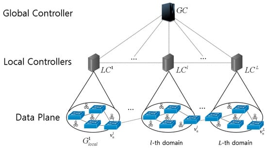
Figure 1.
Network model.
Each LC communicates with the Global Controller (GC) to periodically exchange information on its domain and request path selection for flows beyond its domain area. In addition to maintaining the comprehensive information of all LCs, the GC considers each domain as a virtual node and manages a network graph representing the connections between them, , , where , , and denotes the link between two local domains n and m.
The system model of switch is shown in Figure 2. Let us consider the traffic from this to . Assume that there are k flows, (, arriving at a single queue with infinite and FIFO strategy. Furthermore, the capacity occupied by traffic transmitted to the next node through the service curve is expressed by , and it will be described with cumulative departure traffic.
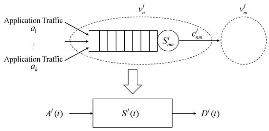
Figure 2.
Switch system model.
The cumulative arrival and departure traffic is represented by stochastic processes and , respectively, for all .
Subsequently, .
The server that deals with traffic is characterized by the service curve .
Each switch system in the local domain l is then simplified with the corresponding , , and , as shown in Figure 2.
3.3. ED Calculation in a Local Domain
Here, we explain the method for calculating the ED for the traffic flow between two switches in a local domain. To generalize the explanation without being limited to a specific switch, the arrival, departure, and service processes at a switch in a local domain are expressed as , , and , respectively, except for the subscripts n, m, and l.
Let the backlog and delay processes in the queue of the switch be and , respectively. Then, we have
In Equation (10), inf(·) represents infimum or greatest lower bound [46]. As in [47], we assume that the arrival process follows a leaky bucket shaper model with bucket ratio and burst parameter b, which is widely applied to define the envelope function that provides the deterministic upper bound of an arrival process. Then, for all , there exist and b satisfying
From Equation (9), we can determine for by assuming that the boundary of exists in the sense that there is a constant rate of service ratio as follows:
We apply the leaky bucket traffic model used in Equation (12) to traffic generation in this study, and we show that existing studies can experimentally simulate traffic similar to real media traffic [48].
Figure 3 shows the relationship between the backlog and delay processes, and , respectively, with respect to , , , , and illustrated above. It should be noted that the service process associates departure process with arrival process .
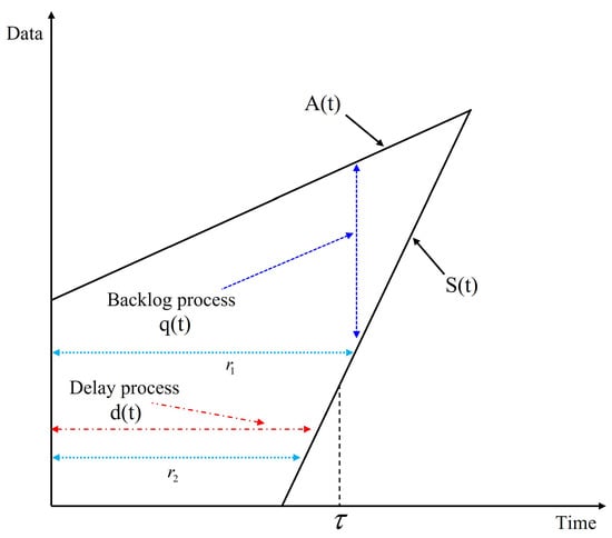
Figure 3.
Representation of the backlog and delay processes.
From Equation (10), it can be written as
The complementary cumulative distribution function of can then be expressed as follows:
We can express the service curve in the min-plus algebra equation as related to departure and arrival to extend to the switches connected between the switches.
where the ⊗ operator is defined as follows:
The arrival and departure at each node within the time interval are described as stochastic behavior of random processes and service curves; for every t with , they can be expressed as follows:
where denotes an error function that provides a bound on the probability that will be violated, and the parameter is used to generate a linear delay boundary in the backlog process where represents the bustiness construct defined in [49] and the characteristics of the service envelope in network calculus. As described in [47], the characteristics of bound business were applied. Consider the case in which packets from a flow are transmitted via W series-connected switches , , ⋯, , as shown in Figure 4, where in the local domain l. Let the service curve of switch be . Then, the service curve passing through W switches is given by [50]
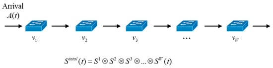
Figure 4.
Traffic process for W traversed switches.
Using the service curve and backlog process characteristics of a single switch defined above, we can obtain the statistical delay bound for consecutively connected switches as follows:
Theorem 1
(Linear Statistical Delay Bound). Let us consider that switches have a constant service rate, , under statistically independent assumptions. An arrival with a traffic service rate and a magnitude b representing the burstiness of traffic is passed through consecutively connected W switches. Assuming a stable situation, the linear statistical delay bound can be calculated as
Proof.
Similar to [51], we can prove the theorem as follows. Let , , , and , respectively, be the delay, arrival, service, and departure processes at the i-th switch along the serial W switches, . From Equation (14), the delay bound at can be expressed as
As is equivalent to , we have
From the definitions of supermartingale and Doob’s maximum linearity and by utilizing the statistical independence of and , we have
Using in Equation (18), the end-to-end latency bound can be written as
Based on the statistical independence of , Equation (23) can be rearranged as follows:
Using the inequality condition, we obtain
Then, we have
Based on being limited by the error function in Equation (17), we obtain the delay as follows:
By differentiating the right-hand side of Equation (27), the optimal value of the delay bound is calculated as
It can be confirmed that the result is given by Equation (29) and . As , can achieve the minimum bound. By contrast, can also achieve the maximum bound. If we say , we can obtain the optimal value as
In addition, we have
The proposed delay bound increases linearly with the number of connected switches, that is, W. The end-to-end delay bound given by Equation (19) can be utilized to determine whether or not the requested delay constraint for the traffic is satisfied.
3.4. Path Selection of a Flow Using ED
As the local switch determines the forwarding port of traffic based on its own flow table, a local switch that does not have a send/receive rule registered in the flow table must request information from the LC regarding which port should forward traffic to the destination. At this time, the LC must handle the flow decision process by considering (1) the presence of a transmission/reception pair in its own management domain and (2) the presence of a destination in a domain other than its own domain.
3.4.1. Case 1: Path Selection of a Flow within a Local Domain
Here, we consider a case that determines the path of a flow in a local domain l, which is represented by a graph as previously defined. When a switch in a local domain l receives a flow request from the source (src) and destination (dst) with traffic type (type) including traffic characteristics and QoS requirements, it forwards the request to . determines the set of possible paths () for the flow, calculates the probabilistic delay bounds for these paths, and selects the best path to satisfy the QoS requirements of the flow.
To find the set of available paths in the local domain, we utilize the multipath A-star algorithm proposed in [52].
For all possible paths in , the delay bound () can be calculated using Equation (19). Subsequently, if the lowest delay bound satisfies the QoS requirements, the path with the lowest delay bound is selected as the flow path. If no path satisfies the delay bound, the flow request is rejected.
3.4.2. Case 2: Path Selection for an Inter-Domain Flow
Step 1: Construct DAG and Set Global Network
For flows that cannot be processed within the LC, the GC must determine the flow by using the DAG between the local domain controller information. In , the graph of the GC is the virtual graph between local domains, the vertex is the local domain, and edge is the edge between the local domains. A pair of inter-domain switches connecting domains l and between each domain is represented by , and the edges are therefore represented by . The GC can construct the connection relationship of the LCs through the inter-domain connection switch (gateway switch) information received from the LC, and reflect it in the global domain graph of the GC.
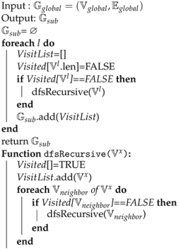
Algorithm 1 describes the construction of the inter-domain connection information and the generation of a DAG for a global inter-domain network to apply topological sorting. First, a variable is initialized to output a set in which the topological ordering of the entire network DAG is completed. The VisitList for the topological order sequence and the Visited variable for checking the visit status are initialized by making a detour based on each domain index. Subsequently, for each unvisited domain vertex, the dfsRecursive() function is called.
The dfsRecursive function treats an unvisited domainvertex as a visit and adds the domainvertex to the VisitList. We then check the visit of each neighbor domain vertex and recursively call dfsRecursive() to the nonvisited neighbor node. This process completes the topological order list from the first domain to the last domain until the entire domain is visited, adding it to , and then calculating the topological order from the next domain index until the last domain index to return the set , which is the final topological ordering.
| Algorithm 1: Construction of DAG set global network. |
 |
Step 2: Flow Path Selection on Multi-Domain
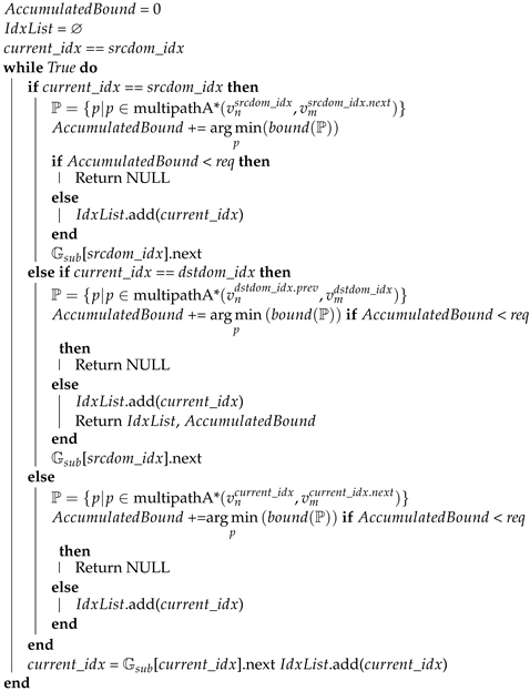
Using the generated topological-order subgraph list, the flow for inter-domain transmission/reception pairs for flows requested by the local switch is determined using Algorithm 2.
First, is initialized to zero to determine whether the QoS is satisfied, and then the domain index () of the switch where the transmission node is located is substituted into . If is the same as the source domain index, the bound between the set of paths between the source switch and the next domain entry switch must be calculated, because the ED bound from the source domain switch in the domain must be calculated. For this calculation, we calculate and then add the minimum boundary to . At this time, the traffic origin node of the source domain node is assumed to be the n-th node of , and is expressed as , and the m-th switch of the next domain in the topological order of the source domain is expressed as .
Subsequently, in the case of inter-domain flow, the minimum boundary of the inlet and outlet switches is calculated, which changes the value after to []. next value, cumulatively calculates the minimum boundary value of the path corresponding to , and determines whether the QoS is satisfied. When the final destination domain arrives, the final domain, like the source domain, calculates the path from the incoming switch to the destination through , calculates it using the minimum boundary, reflects it in the cumulative boundary, and determines whether the QoS is satisfied. The inter-domain flow decision is completed by delivering traffic flow information to the LC corresponding to the index from the source to the cumulative bound.
| Algorithm 2: Inter-domain flow path selection. |
 |
As shown in Algorithm 2, to obtain the path from the source to the destination in the entire requested flow, the path obtained by performing a topological sort is traversed to ensure that the QoS requirements for the traffic type are met. The process in which the GC receives the flow request from the LC and delivers it to the controller related to the flow through the algorithm is shown in Figure 5.
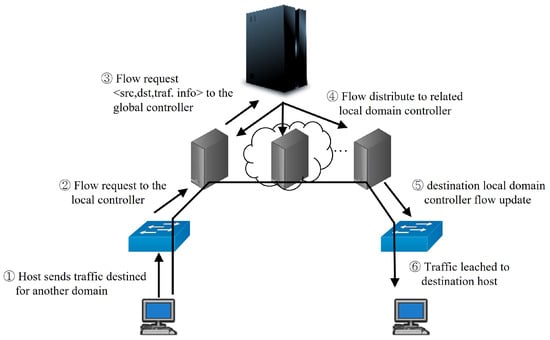
Figure 5.
Path selection procedure for inter-domain flows.
By performing the above process, it is possible to determine a flow that satisfies the QoS requirements within polynomial time when the number of domains is large using the proposed method.
In summary, switches report their queue statistics as defined in the OpenFlow document [53] and the information on arrival and service processes of and which are additionally defined for the proposed method to their LC, periodically or aperiodically. The service rate is set to fixed as in [54], which enables stable estimation of the delay boundary. Each switch calculates the traffic rate based on the current queue static information, i.e., . With the information that switches provide, the LC calculates ED boundaries for source and destination node pairs using Equation (19). Among various methods to transfer metric information between switches and controllers, LLDP control loops can be used. In this case, the overhead of TLV (Type, Length, and Value) fields for the additional information transfer is 8 bytes, which is negligibly small.
Since the times for switches to send their statistic information are not synchronized, the path determined by the LC may not be optimal [55]. However, LLDPs are sent periodically in normal, and immediately when significant changes occur. Thus, we assume that the lack of synchronization problem can be ignored.
When the flow passes through other domains, LC requests the inter-domain path selection process to GC by providing the ED boundary information in its intra-domain and QoS requirements. It is noted that GC maintains the inter-domain paths by DAG based on the topology information received from LCs periodically. For the request of an inter-domain flow, GC determines the inter-domain path satisfying the QoS requirement and passes the path information to LCs connecting the flow.
4. Performance Evaluation
We implemented a network simulator to conduct performance comparisons using Riverbed Modeler 18.9 (formerly OPNET Modeler) with Opendaylight 0.8.4 SDN controllers in order to verify the performance of the proposed method. We compared the proposed method (Proposed) with the Dijkstra algorithm without considering QoS (Dijkstra) and DOLPHIN, which supports QoS in a multi-domain SDN environment [31] (DOLPHIN). We constructed three network topologies using the Abilene, GEANT, and Synth200 topologies with a variable number of hosts per domain, as shown in Figure 6. The number of local hosts per domain was configured to range from 50 to 200.
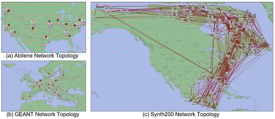
Figure 6.
Simulation topologies.
Table 3 shows the average number of flows according to the topology and the number of hosts. Traffic generation is generated by selecting an arbitrary source host, destination host, and QoS type. As the number of domains increases, the number of flows increases as the number of hosts increases.
Table 3.
Average number of flows according to topology and hosts.
Table 4 lists the traffic types with different delay constraints used in the experiments. There are three traffic types: Best-Effort data (BE Data), Voice over IP (VoIP), and Video on Demand (VOD) with different delay requirements, which were also used in [56,57].
Table 4.
Traffic QoS requirement [56,57].
The BE data traffic does not require any QoS requirements, and is treated with the lowest priority. VoIP traffic has the smallest delay requirement with the highest priority. VOD traffic also has a delay requirement, but is smaller than VoIP, and it has medium priority.
The CDF graph of the Maximum Link Utilization (MLU) for the Abilene topology is shown in Figure 7a. As shown in the figure, it can be seen that the CDF of the graph has a lower link utilization between DOLPHIN and the proposed method with QoS and traffic engineering than the simple path flow selection method without traffic engineering. In addition, it can be seen that the maximum link usage has a lower MLU ratio than DOLPHIN because the alternative path selection is fast for the proposed method.
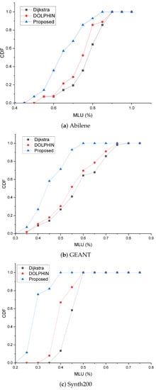
Figure 7.
Link utilization CDF.
The proposed method showed a better performance than the comparison target method in a complex environment. This is because when the topology is complex, the computation process is less complex than that of other methods. In particular, as shown in Figure 7b, traffic engineering is efficiently applied to the Synth200 topology in Figure 7c, indicating that most links are concentrated between 25% and 30%.
The delay CDF graph is the result of deriving traffic delay CDFs in an environment where there are 50 hosts per domain and basic traffic occurs according to the parameters of each topology. Figure 8a shows the delay for the Abilene topology, and it can be seen that the topology is relatively simple, and the delay occurs because of the bottleneck phenomenon that occurs in 70–80% occupied links, as shown in Figure 8a.
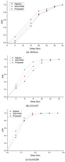
Figure 8.
Maximum delay CDF.
Figure 8b shows the delay for GEANT, and there are relatively many alternative paths to apply traffic engineering, so it is not as simple as the Abilene topology; however, it can be seen that the delay is alleviated. In addition, for Synth200 in Figure 8c, which is a large-scale topology, it can be seen that the delay is low because the link can be evenly distributed. Even in such an environment, the proposed method sets the flow path to which traffic engineering is applied to a lower complexity, indicating that there are more flows with lower latency.
The average delay time graph based on the number of hosts is shown in Figure 9. As the number of hosts increases, traffic saturation increases and traffic congestion increases accordingly. Figure 9a shows the average latency in the Abilene topology. As the alternate paths are almost the same, the increase in latency is observed to be similar as the number of hosts increases. However, Dijkstra support sends traffic without route recalculation, so it can be seen that the increase in latency due to the increase in the number of hosts is greater than in DOLPHIN and the proposed method. Figure 9b shows that the delay is less than that of the Abilene topology because it has more alternative paths than the Abilene topology, with an average delay time in the GEANT topology.
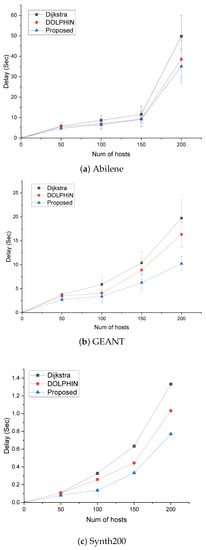
Figure 9.
Average Delay according to the number of hosts.
As shown in the MLU CDF graph in Figure 8, when traffic increases as the number of hosts increases, the delay time of Dijkstra and DOLPHIN with high link saturation is higher than that of the proposed method. As DOLPHIN uses a Dijkstra-based QoS support method, it can be seen that the delay is larger than that of the proposed method because of the influence of processing time due to rediscovery, and the slope of the delay time increase due to host increase is milder. As the Synth 200 topology in Figure 9c has many alternate paths, and the bottleneck is less than other topologies, the latency is smaller than that of the Abilene topology or the GEANT topology. However, as the number of hosts increases, Dijkstra, which does not support QoS, has a relatively high delay time increase rate, whereas in the case of DOLPHIN, a delay occurs by path search and thus has a higher delay than the proposed method.
As the mean of delay is measured in both the inter-and intra-domains, it is necessary to further measure whether end-to-end delay requirements are met to enable accurate performance comparison. First, it can be seen that in the case of Dijkstra, QoS performance is poor in all three topologies. In the case of DOLPHIN supporting QoS, as the number of hosts increases, it can be seen that QoS is provided by the QoS support algorithm, and in the Abile topology of Figure 10a, which has few alternative paths, the QoS performance is almost similar to that of the proposed method. However, in an environment with many alternative paths, we can see that a difference between DOLPHIN and Proposed occurs.
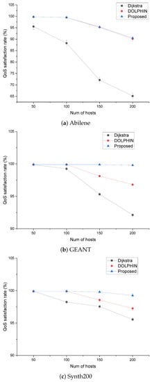
Figure 10.
QoS satisfaction rate according to the number of hosts.
This is because the complexity required to compute the QoS requirements and derive the optimal flows is lower in the case of the proposed method. Figure 10b shows that there is a difference in QoS satisfaction between DOLPHIN and Proposed in the GANT topology, where the number of domains is increased compared with that of Abilene. Compared to Dijkstra, there is a large amount of traffic that satisfies the QoS through the QoS function of DOLPHIN. As the domain increases, the processing time of DOLPHIN increases, particularly for 150 and 200 hosts with a large number of hosts, and the QoS satisfaction rate decreases.
Figure 10c shows that the average latency in the Synth200 topology is reduced compared to that in the GEANT topology because the number of domains increases and there are many alternative paths, so there are fewer bottlenecks. When the QoS is satisfied in this environment, it may be seen that it is lower than GEANT because of the section in which the path is lengthened.
In the case of Dijkstra, as the host increases, the amount of QoS-satisfied traffic decreases owing to the fixed route of traffic transmission, and DOLPHIN increases the amount of satisfied traffic compared to Dijkstra owing to the route of modification according to QoS support. With respect to the proposed method, it can be confirmed that the traffic satisfying QoS requirements is high with a fast processing time of topological sort and path selection considering the delay bound.
Simple Dijkstra approaches that do not support QoS have poor QoS satisfaction because they do not do admission control for traffic with requirements. To increase QoS satisfaction, DOLPHIN and the proposed approaches to which admission control is applied to perform traffic control for flows that do not satisfy the requirements to satisfy QoS priority traffic, drop traffic that does not meet the requirements, and perform admission control for low-priority BE traffic. As shown in Figure 11, in the case of Abilene traffic with low traffic alternative paths, 150 and 200 hosts with high traffic occurrence have high drop rates for traffic that does not meet the requirements. Comparing traffic drops for GEANT and Synth200 traffic, it can be seen that both methods drop for VoIP traffic with high requirement criteria, and the DOLPHIN method shows high drop rates due to the high bandwidth and path calculation complexity for 150 and 200 hosts compared to the proposed method.
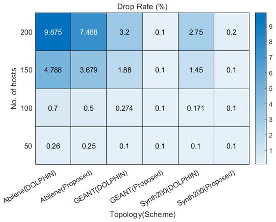
Figure 11.
Representation of the backlog and delay processes.
5. Conclusions
There is a limitation to the application of QoS in a multi-domain environment owing to domain management information imbalance. Compared to traditional networks, SDN enables flexible network configuration management through the control plane, and various studies have been conducted. This study proposed a flow determination method that supports QoS by applying an improved ED calculation in a multi-domain SDN environment. We proposed a DAG-based path selection method for inter-domain flows that satisfies QoS requirements by reducing the variability of determinants within the ED boundaries of the local domain. To verify the performance of the proposed method, comparisons with Dijkstra, without considering QoS and DOLPHIN, which supports QoS in multi-domain environments, were performed using simulations.
Based on the results of the comparison by topology, the performance of DOLPHIN and the proposed method did not differ significantly in Abilene topologies because of the characteristics of the simple Abilene topologies with fewer domains as well as the larger number of alternative paths and Synth200 topologies. In particular, the QoS performance in terms of traffic showed similar characteristics because the alternative paths were limited and the QoS support paths were similar.
Differences were observed in the GEANT and Synth200 topologies because of the differences in performance between the proposed method with computational complexity and DOLPHIN with . Since the proposed method assumes that the time synchronization between the controller and the switch that may occur in the actual environment is consistent, we consider an environment in which there is no time error in the envelope process for efficient delay calculation. However, since this is rare in real-world settings, considering more general environments, we should consider the control traffic overhead and time stamps with less control overhead for considering motivation, such as [55]. In the future, we plan to conduct research on the generalization of deciding factors.
Author Contributions
Conceptualization, G.-m.L., C.-w.L. and B.-h.R.; Data curation, G.-m.L. and B.-h.R.; Funding acquisition, B.-h.R.; Investigation, G.-m.L., C.-w.L. and B.-h.R.; Methodology, G.-m.L., C.-w.L. and B.-h.R.; Project administration, B.-h.R.; Resources, B.-h.R.; Software, G.-m.L. and C.-w.L.; Supervision, B.-h.R.; Validation, G.-m.L.; Writing—original draft, G.-m.L., C.-w.L. and B.-h.R.; Writing—review/editing, B.-h.R. All authors have read and agreed to the published version of the manuscript.
Funding
This work has been supported by the Future Combat System Network Technology Research Center program of Defense Acquisition Program Administration and Agency for Defense Development (UD190033ED).
Institutional Review Board Statement
Not applicable.
Informed Consent Statement
Not applicable.
Data Availability Statement
Not applicable.
Conflicts of Interest
The authors declare no conflict of interest.
Glossary
The following abbreviations are used in this manuscript:
| Abbreviation | Meaning |
| AI | Artificial Intelligence |
| ANP | Analytical Network Process |
| ARX | Autoregressive-exogenous |
| BE | Best Effort |
| BGP | Border Gateway Protocol |
| CDF | Cumulative Distribution Function |
| DAG | Directed acyclic graph |
| DFS | Depth-First Search |
| DQN | Deep Q-Networks |
| EB | Effective Bandwidth |
| ED | Effective Delay |
| ETE | End To End |
| GC | Global Controller |
| LC | Local Controller |
| LLDP | Link Layer Discovery Protocol |
| MLU | Maximum Link Utilization |
| MMOO | Markov-Modulated On-Off |
| MPLS | Multi-Protocol Label Switching |
| NSGA2 | Non-dominated Sorting Genetic Algorithm 2 |
| QoS | Quality of Service |
| RCG | Reliability-aware and minimum-Cost based Genetic |
| SDN | Software Defined Networking |
| TLV | Type, Length, and Value |
| VNF | Virtualized Network Function |
| VOD | Video On Demand |
| VoIP | Voice over IP |
References
- Feamster, N.; Rexford, J.; Zegura, E. The Road to SDN: An Intellectual History of Programmable Networks. SIGCOMM Comput. Commun. Rev. 2014, 44, 87–98. [Google Scholar] [CrossRef]
- Kreutz, D.; Ramos, F.M.V.; Veríssimo, P.E.; Rothenberg, C.E.; Azodolmolky, S.; Uhlig, S. Software-Defined Networking: A Comprehensive Survey. Proc. IEEE 2015, 103, 14–76. [Google Scholar] [CrossRef] [Green Version]
- Keshari, S.K.; Kansal, V.; Kumar, S. A Systematic Review of Quality of Services (QoS) in Software Defined Networking (SDN). Wirel. Pers. Commun. 2021, 116, 2593–2614. [Google Scholar] [CrossRef]
- Ali, J.; Lee, G.m.; Roh, B.h.; Ryu, D.K.; Park, G. Software-Defined Networking Approaches for Link Failure Recovery: A Survey. Sustainability 2020, 12, 4255. [Google Scholar] [CrossRef]
- Morin, C.; Texier, G.; Phan, C. On demand QoS with a SDN traffic engineering management (STEM) module. In Proceedings of the 2017 13th International Conference on Network and Service Management (CNSM), Tokyo, Japan, 26–30 November 2017; pp. 1–6. [Google Scholar]
- Yang, M.; Rastegarfar, H.; Djordjevic, I.B. Physical-layer adaptive resource allocation in software-defined data center networks. IEEE/OSA J. Opt. Commun. Netw. 2018, 10, 1015–1026. [Google Scholar] [CrossRef]
- Froes, W.; Santos, L.; Sampaio, L.N.; Martinello, M.; Liberato, A.; Villaca, R.S. ProgLab: Programmable labels for QoS provisioning on software defined networks. Comput. Commun. 2020, 161, 99–108. [Google Scholar] [CrossRef]
- Wang, R.; Mangiante, S.; Davy, A.; Shi, L.; Jennings, B. QoS-aware multipathing in datacenters using effective bandwidth estimation and SDN. In Proceedings of the 2016 12th International Conference on Network and Service Management (CNSM), Montreal, QC, Canada, 31 October–4 November 2016; pp. 342–347. [Google Scholar]
- Son, J.; Buyya, R. Priority-Aware VM Allocation and Network Bandwidth Provisioning in Software-Defined Networking (SDN)-Enabled Clouds. IEEE Trans. Sustain. Comput. 2019, 4, 17–28. [Google Scholar] [CrossRef]
- Oginni, O.; Bull, P.; Wang, Y. Constraint-Aware Software-Defined Network for Routing Real-Time Multimedia. SIGBED Rev. 2018, 15, 37–42. [Google Scholar] [CrossRef]
- Wu, J.; Qiao, X.; Chen, J. PDMR: Priority-based dynamic multi-path routing algorithm for a software defined network. IET Commun. 2019, 13, 179–185. [Google Scholar] [CrossRef]
- Elbasheer, M.O.; Aldegheishem, A.; Alrajeh, N.; Lloret, J. Video Streaming Adaptive QoS Routing with Resource Reservation (VQoSRR) Model for SDN Networks. Electronics 2022, 11, 1252. [Google Scholar] [CrossRef]
- Li, D.; Wang, X.; Jin, Y.; Liu, H. Research on QoS routing method based on NSGAII in SDN. J. Phys. Conf. Ser. 2020, 1656, 012027. [Google Scholar] [CrossRef]
- Ali, J.; Roh, B.-h. Quality of Service Improvement with Optimal Software-Defined Networking Controller and Control Plane Clustering. CMC-Comput. Contin. 2021, 67, 849–875. [Google Scholar] [CrossRef]
- Kamboj, P.; Pal, S.; Mehra, A. A QoS-aware Routing based on Bandwidth Management in Software-Defined IoT Network. In Proceedings of the 2021 IEEE 18th International Conference on Mobile Ad Hoc and Smart Systems (MASS), Denver, CO, USA, 4–7 October 2021; pp. 579–584. [Google Scholar]
- Mondal, A.; Misra, S. Flowman: Qos-aware dynamic data flow management in software-defined networks. IEEE J. Sel. Areas Commun. 2020, 38, 1366–1373. [Google Scholar] [CrossRef]
- Bastam, M.; RahimiZadeh, K.; Yousefpour, R. Design and Performance Evaluation of a New Traffic Engineering Technique for Software-Defined Network Datacenters. J. Netw. Syst. Manag. 2021, 29, 1–26. [Google Scholar] [CrossRef]
- Bera, S.; Misra, S.; Saha, N.; Sharif, H. Q-Soft: QoS-aware Traffic Forwarding in Software-Defined Cyber-Physical Systems. IEEE Internet Things J. 2021, 9, 9675–9682. [Google Scholar] [CrossRef]
- Ghazizadeh, A.; Akbari, B.; Tajiki, M.M. Joint Reliability-Aware and Cost Efficient Path AllocationFig and VNF Placement using Sharing Scheme. J. Netw. Syst. Manag. 2022, 30, 5. [Google Scholar] [CrossRef]
- Li, J.; Jiang, K.; Wang, J.; Qin, L.; Wei, W. DRNet: QoS-aware Routing for SDN using Deep Reinforcement Learning. In Proceedings of the 2021 IEEE 21st International Conference on Communication Technology (ICCT), Tianjin, China, 13–16 October 2021; pp. 25–30. [Google Scholar]
- Reticcioli, E.; Di Girolamo, G.D.; Smarra, F.; Carmenini, A.; D’Innocenzo, A.; Graziosi, F. Learning SDN traffic flow accurate models to enable queue bandwidth dynamic optimization. In Proceedings of the 2020 European Conference on Networks and Communications (EuCNC), Dubrovnik, Croatia, 16–17 June 2020; pp. 231–235. [Google Scholar]
- Vissers, M.; Busi, I.; Betts, M.; Ong, L.; Zhang, G. SDN architecture for transport networks. In Open Netwing Forum, TR-522; Open Networking Foundation: Palo Alto, CA, USA, 2016. [Google Scholar]
- Kovacevic, I.; Shafigh, A.S.; Glisic, S.; Lorenzo, B.; Hossain, E. Multi-Domain Network Slicing With Latency Equalization. IEEE Trans. Netw. Serv. Manag. 2020, 17, 2182–2196. [Google Scholar] [CrossRef]
- Wang, Y.; Bi, J.; Lin, P.; Lin, Y.; Zhang, K. SDI: A multi-domain SDN mechanism for fine-grained inter-domain routing. Ann. Telecommun. 2016, 71, 625–637. [Google Scholar] [CrossRef]
- Hasija, S.; Mijumbi, R.; Davy, S.; Davy, A.; Jennings, B.; Griffin, K. Domain federation via mpls and sdn for dynamic, real-time end-to-end qos support. In Proceedings of the 2018 Fourth IEEE Conference on Network Softwarization and Workshops (NetSoft), Montreal, QC, Canada, 25–29 June 2018; pp. 177–181. [Google Scholar]
- Yu, H.; Qi, H.; Li, K. WECAN: An efficient west–east control associated network for large-scale SDN systems. Mob. Netw. Appl. 2020, 25, 114–124. [Google Scholar] [CrossRef]
- Böhm, M.; Wermser, D. Multi-Domain Time-Sensitive Networks—Control Plane Mechanisms for Dynamic Inter-Domain Stream Configuration. Electronics 2021, 10, 2477. [Google Scholar] [CrossRef]
- Civanlar, S.; Lokman, E.; Kaytaz, B.; Murat Tekalp, A. Distributed management of service-enabled flow-paths across multiple SDN domains. In Proceedings of the 2015 European Conference on Networks and Communications (EuCNC), Paris, France, 29 June–2 July 2015; pp. 360–364. [Google Scholar]
- Li, Y.; Li, W.; Luo, J.; Jiang, J.; Xia, N. An inter-domain multi-path flow transfer mechanism based on SDN and multi-domain collaboration. In Proceedings of the 2015 IFIP/IEEE International Symposium on Integrated Network Management (IM), Ottawa, ON, Canada, 11–15 May 2015; pp. 758–761. [Google Scholar]
- He, M.; Varasteh, A.; Kellerer, W. Toward a flexible design of SDN dynamic control plane: An online optimization approach. IEEE Trans. Netw. Serv. Manag. 2019, 16, 1694–1708. [Google Scholar] [CrossRef] [Green Version]
- Latif, Z.; Sharif, K.; Li, F.; Karim, M.M.; Biswas, S.; Shahzad, M.; Mohanty, S.P. DOLPHIN: Dynamically optimized and load balanced PatH for INter-domain SDN communication. IEEE Trans. Netw. Serv. Manag. 2020, 18, 331–346. [Google Scholar] [CrossRef]
- Elguea, L.M.; Martinez-Rios, F. An efficient method to compare latencies in order to obtain the best route for SDN. Procedia Comput. Sci. 2017, 116, 393–400. [Google Scholar] [CrossRef]
- Marconett, D.; Yoo, S.B. Flowbroker: A software-defined network controller architecture for multi-domain brokering and reputation. J. Netw. Syst. Manag. 2015, 23, 328–359. [Google Scholar] [CrossRef]
- Joshi, K.D.; Kataoka, K. PRIME-Q: Privacy Aware End-to-End QoS Framework in Multi-Domain SDN. In Proceedings of the 2019 IEEE Conference on Network Softwarization (NetSoft), Paris, France, 24–28 June 2019; pp. 169–177. [Google Scholar]
- Moufakir, T.; Zhani, M.F.; Gherbi, A.; Bouachir, O. Collaborative multi-domain routing in SDN environments. J. Netw. Syst. Manag. 2022, 30, 23. [Google Scholar] [CrossRef]
- Li, D.; Fang, H.; Zhang, X.; Qi, J.; Zhu, Z. DeepMDR: A Deep-Learning-Assisted Control Plane System for Scalable, Protocol-Independent, and Multi-Domain Network Automation. IEEE Commun. Mag. 2021, 59, 62–68. [Google Scholar] [CrossRef]
- Podili, P.; Kataoka, K. TRAQR: Trust aware End-to-End QoS routing in multi-domain SDN using Blockchain. J. Netw. Comput. Appl. 2021, 182, 103055. [Google Scholar] [CrossRef]
- Sun, H.; Chi, X.; Qian, L. Bandwidth estimation for aggregate traffic under delay QoS constraint based on supermartingale theory. Comput. Commun. 2018, 130, 1–9. [Google Scholar] [CrossRef]
- Choi, J. Energy-delay tradeoff comparison of transmission schemes with limited CSI feedback. IEEE Trans. Wirel. Commun. 2013, 12, 1762–1773. [Google Scholar] [CrossRef]
- Burghal, D.; Kim, K.J.; Guo, J.; Orlik, P.V.; Hori, T.; Sumi, T.; Nagai, Y. Multi-Channel Delay Sensitive Scheduling for Convergecast Network. In Proceedings of the 2020 IEEE Wireless Communications and Networking Conference (WCNC), Seoul, Korea, 25–28 May 2020; pp. 1–7. [Google Scholar]
- Ali, J.; Roh, B. Management of Software-Defined Networking Powered by Artificial Intelligence. In Computer-Mediated Communication; Dey, I., Ed.; IntechOpen: London, UK, 2022; Chapter 3; pp. 41–56. [Google Scholar]
- Jacod, J.; Protter, P. Probability Essentials, 2nd ed.; Springer: Berlin/Heidelberg, Germany, 2004. [Google Scholar]
- Ethier, S.N.; Kurtz, T.G. Markov Processes: Characterization and Convergence; John Wiley & Sons: Hoboken, NJ, USA, 2009; Volume 282. [Google Scholar]
- Poloczek, F.; Ciucu, F. Service-martingales: Theory and applications to the delay analysis of random access protocols. In Proceedings of the 2015 IEEE Conference on Computer Communications (INFOCOM), Hong Kong, China, 26 April–1 May 2015; pp. 945–953. [Google Scholar]
- Ciucu, F. Exponential Supermartingales for Evaluating End-to-End Backlog Bounds. ACM SIGMETRICS Perform. Eval. Rev. 2007, 35, 21–23. [Google Scholar] [CrossRef]
- Le Boudec, J.Y.; Thiran, P. Network Calculus: A Theory of Deterministic Queuing Systems for the Internet; Springer: Berlin/Heidelberg, Germany, 2001. [Google Scholar]
- Fidler, M.; Rizk, A. A Guide to the Stochastic Network Calculus. IEEE Commun. Surv. Tutor. 2014, 17, 92–105. [Google Scholar] [CrossRef]
- Thomas, L.; Le Boudec, J.Y.; Mifdaoui, A. On cyclic dependencies and regulators in time-sensitive networks. In Proceedings of the 2019 IEEE Real-Time Systems Symposium (RTSS), Hong Kong, China, 3–6 December 2019; pp. 299–311. [Google Scholar]
- Yaron, O.; Sidi, M. Performance and stability of communication networks via robust exponential bounds. IEEE/ACM Trans. Netw. 1993, 1, 372–385. [Google Scholar] [CrossRef]
- Yu, B.; Chi, X.; Liu, X. Martingale-based Bandwidth Abstraction and Slice Instantiation under the End-to-end Latency-bounded Reliability Constraint. IEEE Commun. Lett. 2021, 26, 217–221. [Google Scholar] [CrossRef]
- Han, Y.; Yao, M.; Yang, Y.; Luo, Y.; XueFang, L. Improving Scalability of Delay Bound with Stochastic Network Calculus. In Proceedings of the GLOBECOM 2020—2020 IEEE Global Communications Conference, Taipei, Taiwan, 7–11 December 2020; pp. 1–6. [Google Scholar]
- Yin, W.; Yang, X. A totally Astar-based multi-path algorithm for the recognition of reasonable route sets in vehicle navigation systems. Procedia-Soc. Behav. Sci. 2013, 96, 1069–1078. [Google Scholar] [CrossRef] [Green Version]
- Foundation, O.N. OpenFlow Switch Specification Version 1.3.5.; Specification; Open Networking Foundation: Palo Alto, CA, USA, 2015. [Google Scholar]
- Miao, W.; Min, G.; Wu, Y.; Huang, H.; Zhao, Z.; Wang, H.; Luo, C. Stochastic performance analysis of network function virtualization in future Internet. IEEE J. Sel. Areas Commun. 2019, 37, 613–626. [Google Scholar] [CrossRef] [Green Version]
- Megyesi, P.; Botta, A.; Aceto, G.; Pescapé, A.; Molnár, S. Challenges and solution for measuring available bandwidth in software defined networks. Comput. Commun. 2017, 99, 48–61. [Google Scholar] [CrossRef]
- ITU-T. ITU-T Recommendation G.1010 (2001), End-User Multimedia QoS Categories; Recommendation; ITU-T: Geneva, Switzerland, 2001. [Google Scholar]
- ITU-T. ITU-T Recommendation Y.1541 (2011), Network Performance Objectives for IP-Based Services; Recommendation; ITU-T: Geneva, Switzerland, 2011. [Google Scholar]
Publisher’s Note: MDPI stays neutral with regard to jurisdictional claims in published maps and institutional affiliations. |
© 2022 by the authors. Licensee MDPI, Basel, Switzerland. This article is an open access article distributed under the terms and conditions of the Creative Commons Attribution (CC BY) license (https://creativecommons.org/licenses/by/4.0/).