Interpretable LSTM Based on Mixture Attention Mechanism for Multi-Step Residential Load Forecasting

Abstract

Residential load forecasting is of great significance to improve the energy efficiency of smart home services. Deep-learning techniques, i.e., long short-term memory (LSTM) neural networks, can considerably improve the performance of prediction models. However, these black-box networks are generally unexplainable, which creates an obstacle for the customer to deeply understand forecasting results and rapidly respond to uncertain circumstances, as practical engineering requires a high standard of prediction reliability. In this paper, an interpretable deep-learning method is proposed to solve the multi-step residential load forecasting problem which is referred to as explainable artificial intelligence (XAI). An encoder–decoder network architecture based on multi-variable LSTM (MV-LSTM) is developed for the multi-step probabilistic-load forecasting. The mixture attention mechanism is introduced in each prediction time step to better capture the different temporal dynamics of multivariate sequence in an interpretable form. By evaluating the contribution of each variable to the forecast, multi-quantile forecasts at multiple future time steps can be generated. The experiments on the real data set show that the proposed method can achieve good prediction performance while providing valuable explanations for the prediction results. The findings help end users gain insights into the forecasting model, bridging the gap between them and advanced deep-learning techniques.

1. Introduction

Modern power systems have become more complex, while suffering from various uncertainties attributed to the high penetration of distributed renewable energy resources [1]. It is essential to ensure reliable power-system and market operation by accurately forecasting techniques [2]. Load forecasting is one of the most effective methods to fight against uncertainty in modern power-system operation and management [3] and plays an important role in economic dispatch, demand response and power market transactions [4]. Traditionally, utility companies focus on the system level or the aggregation level in load forecasting [5]. This aggregated load forecasting is used to arrange the daily startup/shutdown plans of centralized power generation [6].

Nowadays, load forecasting for an individual residential customer has become increasingly important in smart-grid planning and operation [7]. To better use renewable energy, load forecasting for residential customers can help energy storage systems to make the best decisions on charging/discharging operation. A home energy-management system can improve energy efficiency by shifting the flexible load such as air-conditioner systems and balancing demand with the fluctuating supply of renewable energy. Furthermore, residential load forecasting can support utilities to develop more reasonable demand-response strategies, and reduce grid operating costs [8]. With the volatility in distributed energy and load in households, it is quite challenging to precisely predict an individual load, which hinders the applications of residential load forecasting, i.e., peer-to-peer energy trading [9].

The availability of smart meters that provide fine-grained data facilitates residential load forecasting [10]. Many open data sources have also promoted this research. Compared with the aggregated load, the electric load of a individual household not only depends on external environmental factors such as weather and special events [11], but is also highly related to the lifestyle and consumption patterns of residents [12]. The load curve of an individual household will inevitably show greater volatility [13]. In addition, due to the sparse deployment of data collection sensors and inevitable errors, collected data may often be approximate or inaccurate. At the same time, load series often have long-term dependence, such as weekly or daily seasonal patterns. There are complex or even uncertain nonlinear relationships between internal or external factors and future load demand. It is difficult to accurately capture these relationships in a model for prediction.

As the amount and dimensions of smart-grid data increase, the performance of traditional machine-learning methods is becoming worse [3]. Traditional machine-learning methods find it difficult to obtain good accuracy in residential load forecasting, where most of these methods use pre-defined nonlinear forms and may not be able to accurately capture nonlinear relationships [14]. Recently, deep neural networks (DNN) have been increasingly used for residential load forecasting. Shi et al. [15] proposed an LSTM neural network based on pooling for residential load forecasting. They studied a 920-customer case in Ireland and proved that the recurrent neural network(RNN)-based forecasting method is better than the benchmark method, including autoregressive integrated moving average (ARIMA) model and support vector regression (SVR). Kong et al. [3] also proposed a deep-learning prediction framework based on LSTM to predict single-step household load. Wang et al. [16] proposed a gated recurrent unit (GRU) model to predict the residential load of the next day. Wang et al. [5] took residential and small-and-medium-enterprise customers as the research object and proposed a probabilistic individual load forecasting model based on the pinball loss function and LSTM, aiming to quantify the uncertainty of individual user load. Yang et al. [17] proposed a probabilistic-load forecasting framework based on deep ensemble learning, which uses customer classification and multi-task representation learning to improve the quantitative performance of the uncertainty of an individual load. The above results show that the use of deep-learning technology can provide better performance on this issue. In particular, RNNs specifically designed for sequence modeling have powerful performance improvements on this issue.

A key factor for a successful deep neural network is its capability of highly nonlinear approximation with multiple layers [18]. However, this makes it difficult to explain how the model reaches its expressive performance. If a forecasting model cannot provide an explanation understandable by humans, it will be difficult for end users to trust the prediction result, which creates an obstacle for load shifting. Therefore, in order to make the residential load-forecasting model based on deep learning trustworthy, it is critical to develop a new technique for explanations that are understandable by humans.

Currently, an attention mechanism [19] is often used to explain predictions for various temporal prediction tasks. The naive attention mechanism only has a certain degree of interpretability [20]. When the attention layer is used for each time step, the attention scores can be interpreted as the importance of different time steps. Ma et al. [21] proposed a vessel collision risk early-warning model based on an attention mechanism and bidirectional LSTM. The attention mechanism was used to quantify the impact of motor behavioral characteristics at a certain time step, on future risk. When the attention layer is used for each variable, the attention scores can be interpreted as the importance of different features. Liao et al. [22] proposed a graph neural network model combining multimodal information for taxi demand prediction. An attention mechanism is used to model the correlation between multimodal features (weather, events or text, etc.) and taxi demand. However, time-series prediction contains many different types of input features at each time step. Single attention mechanism does not allow us to understand the importance of each feature at each time step, and cannot distinguish the contribution of a single variable to the prediction result. To address this, a new interpretable time-series model based on two sets of attention was developed by Choi et al. [23]. The model trains two RNN sequences in reverse time sequence, and each sequence takes temporal importance and variable importance into consideration, respectively. Guo et al. [24] proposed an interpretable MV-LSTM with a mixture attention mechanism for multi-variate time-series forecasting. A mixture attention mechanism firstly determines the variable-wise temporal importance, and then weighs the last hidden state that belongs to each variable to determine the importance of every variable. Li et al. [25] implemented a multi-variate LSTM on a memristor system for residential load forecasting. However, these methods can only predict one time step and cannot realize interpretable multi-step load forecasting. Lim et al. [26] proposed a temporal fusion transformer for multi-step time-series forecasting. Toubeau et al. [27] proposed a model based on an attention mechanism and encoder–decoder structure for area control-error prediction. This two models use a variable selection network to choose important variables, but cannot capture the variable-wise temporal dynamics.

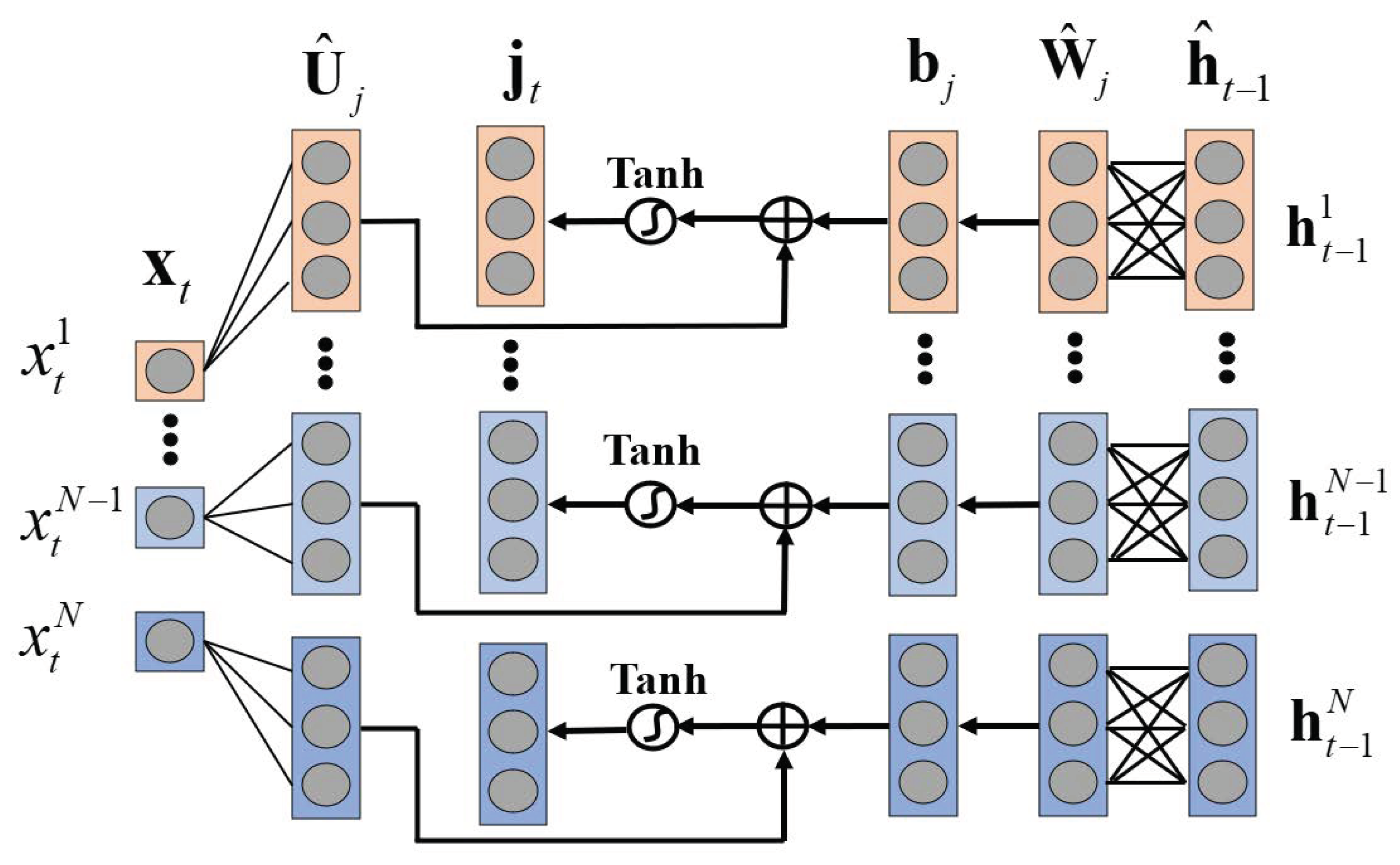
In this paper, we use a mixture attention mechanism to explain the forecasting results of residential load that can characterize the temporal dynamics of different input variables and improve the prediction performance. More importantly, the leverage of the mixture attention mechanism provides two valuable interpretations of variables and time steps for residential load forecasting. Due to the popularity of distributed energy in households, future load demand fluctuates significantly. Traditional point forecasting cannot fully quantify the uncertainty of residential load demand. Therefore, we use probabilistic forecasting to output the quantiles of future residential load. Unlike traditional point forecasting, which only outputs the expected value of future loads, quantile forecasting can explore the distribution of future loads [28]. In addition, in order to work with long-term future time series, the encoder–decoder architecture was established to implement multi-step ahead forecasting, in which the quantile outputs for future multiple time steps can be predicted simultaneously. The established interpretable multi-step probabilistic forecasting model expands the capacity of the learning model for future decision making.

The remainder of this paper is structured as follows. The multi-step residential load forecasting problem is described in Section 2. Section 3 introduces the working principle of the interpretable multi-step load forecasting model. Section 4 introduces the experiments for residential load forecasting and discusses the experimental results and model interpretability for residential load forecasting. Section 5 draws a conclusion.

2. Problem Formulation

Let the time-series observation of the residential load of the i-th customer at time step t be represented by $y_{i,t}$. The general load forecasting aims to predict the future load time series $[y_{i,t_0},y_{i,t_0+1},\cdots y_{i,t_0+T}]:={\mathbf{y}}_{i,t_0:t_0+T}$ given its past $[y_{i,0},y_{i,1},\cdots y_{i,t_0-1}]:={\mathbf{y}}_{i,0:t_0-1}$ with respect to customer i. $t_0$ is the reference time from which the actual $y_{i,t}$ is unknown at prediction time. In addition, ${\mathbf{z}}_{i,0:t_0+T}$ are covariates that are known for the entire time period $0:t_0+T$, e.g., hour of the day or weather forecasting.

Quantile regression can predict the conditional distribution of a target variable without assuming specific parametric distribution. It can flexibly represent the uncertainty of future loads and give different possible load demands. Therefore, quantile load forecasting is useful to optimize decision making for home energy-management systems. In this paper, we use probabilistic quantile regression to perform quantile prediction ${\widehat{\mathbf{y}}}_{i,t}={\left\{{\widehat{y}}_{i,t}^q\right\}}_{q\in Q}$ for target quantile set Q at each prediction time step $t\in [t_0,t_0+T]$. Multi-step quantile prediction is obtained by the following equation:

$${\widehat{\mathbf{y}}}_{i,t_0:t_0+T}=f({\mathbf{y}}_{i,0:t_0-1},{\mathbf{z}}_{i,0:t_0+T})$$

(1)

For notation simplicity, we omit the subscript i of the customer unless explicitly required. Then, to easily manage different types of variables, we represent the input at each time step as follows:

$${\mathbf{x}}_t=[y_{t-1}\oplus {\mathbf{z}}_t],{\mathbf{X}}_t={[{\mathbf{x}}_1,{\mathbf{x}}_2,\cdots {\mathbf{x}}_t]}^{\top }$$

(2)

where $[·\oplus ·]$ represents concatenation. We try to predict the quantile of next $T+1$ time steps from $t_0$ for all time series. To train a forecasting model, multiple training samples were created by choosing a window $[0,t_0+T]$ with consecutive starting time slots. To illustrate it clearly, the time ranges $[0,t_0-1]$ and $[t_0,t_0+T]$ corresponding to ${\mathbf{X}}_t$ are called the condition and the prediction windows, respectively.

3. Interpretable Forecasting Model

3.1. Multi-Variable LSTM Cell

Unlike using Bayesian learning for achieving the interpretability of residential load forecasting, as in [29], the mixture attention mechanism is proposed which can be recognised as a multi-variable interpretable LSTM neural network. When making predictions with multiple input variables using a traditional LSTM, different dynamics of each feature are indistinguishable after being processed by different gates [24]. Moreover, there is no correspondence between each input variable and each hidden state for the input-to-hidden transition. MV-LSTM can capture this transition relationship of input variables and hidden states.

For a cell of MV-LSTM, the hidden-state matrix at timestep t can be defined as ${\widehat{\mathbf{h}}}_t={[{\mathbf{h}}_t^1,{\mathbf{h}}_t^2,\cdots {\mathbf{h}}_t^N]}^{\top }\in {\mathbb{R}}^{N\times d}$, where N is the number of input features and ${\mathbf{h}}_t^n\in {\mathbb{R}}^d$ is the n-th vector of the hidden-state matrix corresponding to input $x_t^n$. The input-to-hidden transition can be defined as ${\widehat{\mathbf{U}}}_j={[{\mathbf{U}}_j^1,{\mathbf{U}}_j^2,\cdots {\mathbf{U}}_j^N]}^{\top }\in {\mathbb{R}}^{N\times d\times d_0}$, where ${\mathbf{U}}_j^n\in {\mathbb{R}}^{d\times d_0}$ and $d_0$ are the dimensions of the input features with respect to each individual variable at each timestep. The hidden-to-hidden transition is defined as ${\widehat{\mathbf{W}}}_j={[{\mathbf{W}}_j^1,{\mathbf{W}}_j^2,\cdots {\mathbf{W}}_j^N]}^{\top }\in {\mathbb{R}}^{N\times d\times d}$, where ${\mathbf{W}}_j^n\in {\mathbb{R}}^{d\times d}$. The updating process of hidden update ${\mathbf{j}}_t$ is shown in Figure 1. The specific calculation process is:

$$\begin{array}{ccc}\hfill {\mathbf{j}}_t& =& tanh\left({\widehat{\mathbf{W}}}_j⊛{\widehat{\mathbf{h}}}_{t-1}+{\widehat{\mathbf{U}}}_j⊛{\mathbf{x}}_t+{\mathbf{b}}_j\right)\hfill \end{array}$$

(3)

where ${\mathbf{j}}_t={[{\mathbf{j}}_t^1,{\mathbf{j}}_t^2,\cdots {\mathbf{j}}_t^N]}^{\top }\in {\mathbb{R}}^{N\times d}$ and ${\mathbf{j}}_t^n$ is the update-process-based element of the hidden states regarding input $x_t^n$. ⊛ is a tensor-based operator for the element-wise product of two tensors, i.e., ${\widehat{\mathbf{U}}}_j⊛{\mathbf{x}}_t={[{\mathbf{U}}_j^1{\mathbf{x}}_t^1,{\mathbf{U}}_j^1{\mathbf{x}}_t^1,\cdots {\mathbf{U}}_j^N{\mathbf{x}}_t^N]}^{\top }\in {\mathbb{R}}^{N\times d}$. MV-LSTM also has the input gate ${\mathbf{i}}_t$, the forget gate ${\mathbf{f}}_t$, the output gate ${\mathbf{o}}_t$ and the memory cell ${\mathbf{c}}_t$, which are defined as follows:

$$\begin{array}{ccc}\hfill {\mathbf{i}}_t& =& \sigma \left({\widehat{\mathbf{W}}}_j^{{\mathbf{i}}_t}⊛{\widehat{\mathbf{h}}}_{t-1}+{\widehat{\mathbf{U}}}_j^{{\mathbf{i}}_t}⊛{\mathbf{x}}_t+{\mathbf{b}}_j^{{\mathbf{i}}_t}\right)\hfill \end{array}$$

(4)

$$\begin{array}{ccc}\hfill {\mathbf{f}}_t& =& \sigma \left({\widehat{\mathbf{W}}}_j^{{\mathbf{f}}_t}⊛{\widehat{\mathbf{h}}}_{t-1}+{\widehat{\mathbf{U}}}_j^{{\mathbf{f}}_t}⊛{\mathbf{x}}_t+{\mathbf{b}}_j^{{\mathbf{f}}_t}\right)\hfill \end{array}$$

(5)

$$\begin{array}{ccc}\hfill {\mathbf{o}}_t& =& \sigma \left({\widehat{\mathbf{W}}}_j^{{\mathbf{o}}_t}⊛{\widehat{\mathbf{h}}}_{t-1}+{\widehat{\mathbf{U}}}_j^{{\mathbf{o}}_t}⊛{\mathbf{x}}_t+{\mathbf{b}}_j^{{\mathbf{o}}_t}\right)\hfill \end{array}$$

(6)

$$\begin{array}{ccc}\hfill {\mathbf{c}}_t& =& {\mathbf{f}}_t\odot {\mathbf{c}}_{t-1}+{\mathbf{i}}_t\odot {\mathbf{j}}_t\hfill \end{array}$$

(7)

where ⊙ denotes element-wise multiplication. Finally, the hidden-state matrix corresponding to time step t is computed by:

$$\begin{array}{ccc}\hfill {\widehat{\mathbf{h}}}_t& =& {\mathbf{o}}_t\odot tanh\left({\mathbf{c}}_t\right)\hfill \end{array}$$

(8)

3.2. Mixture Attention for Interpretable Prediction

In general, the attention mechanism can easily be harnessed to weigh hidden states at different time steps which can give the overall temporal importance of input features. However, it is difficult to extract the variable-wise temporal importance, which can measure the change in single-feature importance over time. By applying the MV-LSTM, we obtain the sequence of the hidden-state matrices $\{{\widehat{\mathbf{h}}}_1,{\widehat{\mathbf{h}}}_2,\cdots {\widehat{\mathbf{h}}}_t\}$, where the sequence of hidden states specific to feature n is denoted by $\{{\mathbf{h}}_1^n,{\mathbf{h}}_2^n,\cdots {\mathbf{h}}_t^n\}$. MV-LSTM leverages different attention mechanisms among the variable and variable-wise temporal importance. The idea of the mixture attention mechanism is as follows.

Firstly, we apply variable-wise temporal attention to the hidden states of the latest $t_0$ time steps corresponding to each variable to obtain the summary history information of each variable. In particular, the context vector ${\mathbf{g}}_t^n$ of the variable-wise temporal attention mechanism regarding ${\mathbf{x}}^n$ is defined as:

$${\mathbf{g}}_t^n=\sum _{k=1}^{t_0}{\alpha }_{t,k}^n{\mathbf{h}}_{t-t_0+k}^n$$

(9)

where the temporal attention weight ${\alpha }_{t,k}^n$ is defined as:

$${\alpha }_{t,k}^n=\frac{\exp \left(f_n\left({\mathbf{h}}_{t-t_0+k}^n\right)\right)}{{\sum }_{j=1}^{t_0}\exp \left(f_n\left({\mathbf{h}}_{t-t_0+j}^n\right)\right)}$$

(10)

and $f_n(·)$ is a feedforward neural network.

Then, we obtain the variable state ${\mathbf{s}}_t^n$ by concatenating ${\mathbf{h}}_t^n$ and ${\mathbf{g}}_t^n$:

$${\mathbf{s}}_t^n=[{\mathbf{h}}_t^n\oplus {\mathbf{g}}_t^n]$$

(11)

In each prediction time step, the variable states of all input variables are jointly used to construct variable attention, thereby facilitating the representation of variable importance. The variable attention weight is calculated by:

$${\beta }_t^n=\frac{\exp \left(f_s\left({\mathbf{s}}_t^n\right)\right)}{{\sum }_{k=1}^N\exp \left(f_s\left({\mathbf{s}}_t^k\right)\right)}$$

(12)

where $f_s(·)$ is also a feedforward neural network.

For residential load forecasting, we obtain the prediction interval by simultaneously generating several quantiles at each prediction time step. One quantile prediction is calculated by weighted linear transformation:

$$\begin{array}{ccc}& & {\mu }_n^q={\mathbf{W}}_{\mu }^q{\mathbf{s}}_t^n+{\mathbf{b}}_{\mu }^q\hfill \end{array}$$

(13)

$$\begin{array}{ccc}& & {\widehat{y}}_t^q=\sum _{n=1}^N{\beta }_t^n{\mu }_n^q\hfill \end{array}$$

(14)

where ${\mathbf{W}}_{\mu }^q$, ${\mathbf{b}}_{\mu }^q$ are the coefficients with respect to the q quantile. Note that predictions are only generated for the prediction window, that is, $t\in [t_0,t_0+T]$.

3.3. Interpretable Encoder–Decoder Network

In this paper, our goal is to achieve a high-performance prediction model of residential multi-step load while obtaining the model’s internal explanations. To address this issue, we proposed an encoder–decoder network architecture based on MV-LSTM and a mixture attention mechanism. Figure 2 shows the architecture of our proposed interpretable multi-step probabilistic load forecasting model.

The encoder network and the decoder network are used to process the input data of the condition window and the prediction window, respectively [30]. Furthermore, the same architecture is used in the encoder and decoder, and the weights between them are shared. The encoder encodes all historical information in the condition window ${\mathbf{X}}_{t_0-1}$ into a hidden state ${\widehat{\mathbf{h}}}_{t_0-1}$. ${\widehat{\mathbf{h}}}_{t_0-1}$ is transmitted to the prediction window as the initial state of the decoder. The initial state of the encoder ${\widehat{\mathbf{h}}}_0$ is initialized to zero. In the decoder, the prediction is generated recursively, that is, the network output of the last time step is input to the network as feedback at the next time step. For the prediction window, we can feedback the $0.5$ quantile ${\widehat{y}}_t^{0.5}$ to the input of the next time step. In addition, ${\widehat{y}}_{t_0-1}^{0.5}$ is initialized by $y_{t_0-1}$.

We use the teacher forcing training strategy to train the interpretable network. During training, the value of $y_t$ is known within the prediction window. Therefore, the basic truth of the target sequence is input to the decoder for training. In the test phase, for $t\in [t_0,t_0+T]$, $y_t$ is unknown. We use ${\widehat{y}}_t^{0.5}$ generated in the previous step as the input for the later time step.

3.4. Model Interpretability

Feature importance or variable importance is the most common form in interpretable machine learning, which explains the relationship between those variables that produce predictions, providing important information about predictions. Analyzing the relationship between load consumption and factors such as weather conditions (temperature, humidity) and time-dependent variables (day of week, time of day) can help utilities analyze changes in electricity demand. In fact, the effects of these variables on the load are complex, nonlinear and interdependent. Moreover, different variables provide different contributions to the predicted outcome. The importance of variables also changes at different prediction time steps. The variable attention mechanism in our model provides these insights. The predicted outcome in (14) is a weighted sum of variable states ${\mathbf{s}}_t^n$. ${\beta }_t^n$ is the weighting coefficient in prediction time step t, which represents the contribution of the variable to the output.

Next, we quantify the global variable importance by individual variable attention weights. Specifically, we aggregate the variable attention weight of each input variable on the training set to extract general insights about the global variable importance. The global variable importance $I^n$ can be obtained by:

$$I^n=\frac{{\sum }_{m=1}^M{\sum }_{t=t_0}^{t_0+T}{\beta }_t^{m,n}}{M(T+1)}$$

(15)

where $I_n\in R_{+}$ and ${\sum }_{n=1}^N{I}_n=1$, and M represents the number of samples in traing set.

Temporal importance analysis can help us extract the persistent temporal pattern and understand the temporal dependence in different variables in the dataset. In this paper, the variable-wise temporal importance is referred as the impact from the last $t_0$ time steps of a single feature, which is defined by $\mathbf{T}=\{T_1^1,\cdots T_1^{t_0};T_2^1,\cdots T_2^{t_0};\cdots ;T_N^1,\cdots T_N^{t_0}\}$, where $T_n^k\in R_{+}^{t_0}$ and ${\sum }_{k=1}^{t_0}{T}_n^k=1$. We quantify the variable-wise temporal importance by aggregating the temporal attention weights of different variables for each prediction time step on the training set. The variable-wise temporal importance $T_k^n$ can be obtained by:

$$T_k^n=\frac{{\sum }_{m=1}^M{\sum }_{t=t_0}^{t_0+T}{\alpha }_{t,k}^{m,n}}{M(T+1)}$$

(16)

4. Case Study

4.1. Data Description and Preparation

In this paper, we used one residential load consumption data set without missing values collected from 78 residential customers near the airport in Western Victoria, Australia to evaluate the performance of proposed model for residential load forecasting. Each customer contains 35,040 measurements with half-hour resolution from 1 January 2017 to 31 December 2018. In addition, we obtained weather observations and forecasting data from the nearest weather station. A linear interpolation technique was used to estimate missing measurements.

In our proposed model, we consider three types of input: auto-regressive variable—i.e., load consumption observation, time-related variables, and weather information. We take month, day of the week, hour and holiday, etc. to be four variables as the time-related variables, each of which is a real-valued input. The weather information includes seven real-valued variables: temperature, relative humidity, dew point, wind speed, cloud type, visibility and precipitation. In view of the magnitude difference between the load series of different customers, we separately applied 0–1 standardization to input the variables of each customer.

4.2. Baseline Methods and Training Procedure

We compared our proposed method with multiple multi-step forecasting methods.

(1)

Gradient boosting quantile regression (GBQR): GBQR is a tree ensemble method based on boosting. We used the Python package Scikit-learn [31] to implement GBQR with quantile loss function and the number of trees was set to 500. MultiOutputRegressor of Scikit-learn was used to obtain multistep forecasting results. It is worth noting that MultiOutputRegressor trains a model for each step of prediction.

(2)

Quantile regression forest (QRF): QRF is also an ensemble learning approach for regression and classification tasks which obtains prediction results by creating different decision trees. QRF is implemented by the Python package Scikit-garden [32] and the number of trees was also set to 500. QRF was used to build a model for each prediction step.

(3)

Multi-layer perceptron (MLP): An MLP with three hidden layers and a Relu activation function was used for load forecasting for all future time steps. The loss function is the average pinpall loss function.

(4)

Encoder–decoder: The encoder–decoder model contains two LSTMs, an encoder LSTM and a decoder LSTM [33]. The encoder LSTM encodes the input sequence as a feature representation. The decoder LSTM uses the context vector generated by the encoder LSTM as its initial hidden state and extracts its own input combined with the previous step estimate to iteratively generate predictions at each time step.

(5)

Attention encoder–decoder: The attention encoder–decoder model is a prediction model that combines encoder–decoder and temporal attention mechanism [33].

In our experiment, we focused on the load forecasting of the next day (i.e., 48 time steps) using the information of the previous day (i.e., 48 time steps) and we computed quantiles with $q\in Q=\{0.01,0.05,0.1,0.25,0.5,0.75,0.9,0.95,0.99\}$. We implemented our proposed method and other deep-learning baseline methods using Pytorch. We divided the data set into training, validation, and test sets with a ratio of 70/15/15. We used the Adam algorithm with a mini-batch size of 32 to train the model. We used gradient clipping to avoid large gradients in the iteration. The maximum training epoch was 100, and we used early stopping on the validation data set to avoid overfitting. The performance of deep models is heavily dependent on hyperparameter selection. We selected the best hyperparameters through a grid search. The following is the search scope of all hyperparameters:

• The size of a fully connected layer or LSTM of baseline methods $\{16,32,64,128\}$.
• LSTM size of our proposed method $\{10,20,30,40\}$.
• Dropout rate $\{0,0.2,0.5\}$.
• Learning rate $\{0.0001,0.001,0.01\}$.
• Maximum gradient norm $\{0.01,1.0,100.0\}$.

In this paper, the loss function is defined as the average pinball loss over the quantiles of all prediction time steps, which was calculated as follows:

$$\begin{array}{ccc}\hfill & & L(\mathbf{y},\widehat{\mathbf{y}},Q)=\frac{1}{M\times (T+1)\times \left|Q\right|}\sum _{s_i\in \mathrm{\Omega }}\sum _{y_t\in s_i}\sum _{q\in Q}P(y_t,{\widehat{y}}_t^q,q)\hfill \end{array}$$

(17)

$$\begin{array}{ccc}& & P(y_t,{\widehat{y}}_{t,q},q)=max((q-1)(y_t-{\widehat{y}}_t^q),q(y_t-{\widehat{y}}_t^q))\hfill \end{array}$$

(18)

where $\mathrm{\Omega }$ represents the training set, $s_i$ represents one sample of the training set, $\left|Q\right|$ is the size of quantile set, and P is the pinball loss function.

4.3. Evaluation Criteria

4.3.1. Point Forecasting

Point forecasting is the primary objective of residential load forecasting, and is very critical to the day-ahead scheduling of home energy-management systems. The quantile regression model can obtain the prediction results of different quantiles. Among them, when $q=0.5$, $P(y_t,{\widehat{y}}_{t,q},q)$ is equivalent to the mean absolute error (MAE) loss. Accordingly, the prediction result of the $0.5$-th quantile ${\widehat{y}}_t^{0.5}$ can be approximated as the point forecasting value. We employed three metrics to measure the performance of point forecasting on the test set, including the root mean square error (RMSE), the MAE, and the mean absolute percentage error (MAPE). They were formulated as follows:

$$\begin{array}{ccc}& & RMSE=\sqrt{\frac{1}{T^{\prime }}{\displaystyle \sum _{t=1}^{T^{\prime }}}{(y_t-{\widehat{y}}_t^{0.5})}^2}\hfill \end{array}$$

(19)

$$\begin{array}{ccc}& & MAE=\frac{1}{T^{\prime }}\sum _{t=1}^{T^{\prime }}|y_t-{\widehat{y}}_t^{0.5}|\hfill \end{array}$$

(20)

$$\begin{array}{ccc}& & MAPE=\frac{100\%}{T^{\prime }}\sum _{t=1}^{T^{\prime }}\frac{|y_t-{\widehat{y}}_t^{0.5}|}{|y_t|}\hfill \end{array}$$

(21)

where $T^{\prime }$ is the total number of time steps of test set.

4.3.2. Probabilistic Forecasting

Probabilistic forecasting based on quantile regression can obtain the variation interval of the quantity to be predicted. Interval prediction is usually evaluated in terms of reliability and sharpness. Reliability measures how far the quantile deviates from the actual observed value. Sharpness describes the width of the prediction interval. The average pinball score on the test set is a composite measure of reliability and sharpness and is expressed as follows:

$$\begin{array}{c}\hfill Pinball=\frac{1}{\left(T^{\prime }\right)\times \left|Q\right|}\sum _{t=1}^{T^{\prime }}\sum _{q\in Q}P(y_t,{\widehat{y}}_t^q,q)\end{array}$$

(22)

In addition, the average Winkler score is also a composite index that takes into account both the coverage probability and width of the prediction interval. For a confidence interval of $(1-ϵ)\times 100\%$, the Winkler score for one time step can be computed as follows:

$$\begin{array}{c}\hfill Winkle{r}_t=\left\{\begin{array}{cc}{\delta }_t\hfill & L_t\le y_t\le U_t\hfill \\ {\delta }_t+2\left(L_t-y_t\right)/ϵ\hfill & y_t<L_t\hfill \\ {\delta }_t+2\left(y_t-U_t\right)/ϵ\hfill & y_t>U_t\hfill \end{array}\right.\end{array}$$

(23)

where ${\delta }_t=U_t-L_t$ is the width of interval at time step t, and $L_t=y_t^{ϵ/2}$ and $U_t=y_t^{1-ϵ/2}$ are the lower and upper bounds, respectively. $ϵ=0.02,0.1,0.2,0.5$ were considered for computing the Winkler score in this paper. A lower Winkler score means better interval estimation.

4.4. Forecasting Results

In this subsection, we present the performance comparison results of the proposed method with other baseline methods in point forecasting and probabilistic forecasting.

Table 1. Performance comparison of different methods for point forecasting.

Methods	RMSE	MAE	MAPE
GBQR	0.2412	0.1291	0.4697
QRF	0.2450	0.1243	0.4869
MLP	0.2521	0.1392	0.4901
Encoder–decoder	0.2351	0.1173	0.4675
Attention encoder–decoder	0.2403	0.1281	0.4803
Proposed method	0.2240	0.1102	0.4438

shows the comparison results of the point forecasting performance of different methods. Compared with the baseline methods, our proposed model obtains the best prediction performance, which shows the superiority of mixture attention on the variable-wise hidden states. Since the multi-step forecasting strategy along the time direction can easily utilize the known information in the future, the encoder–decoder model provides the second-best result. It is worth noting that the attention encoder–decoder model does not improve prediction performance relative to the encoder–decoder model. This shows that the temporal attention mechanism acting on a recurrent layer cannot extract the variable-wise important information and find salient features. Compared to MLP, GBQR and QRF provides better results. We built a prediction model for each future time step for tree models, which is inefficient and time-consuming, so they are not very applicable in practical applications.

Quantile forecasting at different probability levels show insights into future demand scenarios, which have important implications for electricity risk management. To quantify the performance of probabilistic forecasting, we present the average pinball scores and Winkler scores at different reliability levels of different methods in

Table 2. Performance comparison of different methods for probabilistic forecasting.

Methods	Pinball	Winkler
		$\mathbf{\beta }=\mathbf{0}.\mathbf{02}$	$\mathbf{\beta }=\mathbf{0}.\mathbf{1}$	$\mathbf{\beta }=\mathbf{0}.\mathbf{2}$	$\mathbf{\beta }=\mathbf{0}.\mathbf{5}$
GBQR	0.0321	1.3167	0.8754	0.6548	0.4269
QRF	0.0387	1.3283	0.9021	0.6731	0.4381
MLP	0.0335	1.2993	0.8241	0.6423	0.4193
Encoder–decoder	0.0296	1.1867	0.7694	0.6007	0.3911
Attention encoder–decoder	0.0314	1.1871	0.7691	0.5994	0.3920
Proposed method	0.0281	1.0023	0.7403	0.5824	0.3782

. Likewise, our proposed method can generate better quantile predictions, showing high reliability and sharpness. This is because the mixture attention mechanism can effectively capture the uncertainty brought by different variables and very suitable for highly fluctuating residential load data. It can also be seen that the performance of the deep-learning models is better compared to the tree models. This suggests that deep learning is well-suited for probabilistic forecasting, producing tighter and more reliable prediction intervals.

In Figure 3, we show the results of quantile forecasting for a randomly selected residential customer in a week. The black point shows the actual load consumption values and the red curve shows the median (0.5 quantile) prediction result. Dark blue and light blue represent the $50\%$ and $90\%$ prediction intervals, respectively. This customer has a high load demand in the morning and evening, and low load demand at other times, which may be due to sleeping or going out. The consumption profile of this household customer has high volatility in the high-load-demand time due to the variability in residential consumer behavior. It can be seen that the prediction interval basically covers the actual load, and the median is very close to the actual load. It is worth emphasizing that the accurate prediction of peak load is an important factor for the operation of home energy-management systems, and satisfactory prediction results can be obtained using the proposed forecasting model based on the mixture attention mechanism. This indicates that the load volatility and temporal pattern of the load consumption profile are well-captured by the model.

4.5. Interpretability Analysis on Variable Importance

After analyzing the performance of the model, we elaborated on the interpretability of the proposed model. To interpret the prediction results, we first calculated the global variable importance of the mixture attention mechanism by Equation (15). Variable attention can distinguish the significance of variables by the attention score. The global variable importance results are shown in Figure 4. The horizontal axis represents the input variable, and the vertical axis is the global feature importance score of the input variable. It can be seen that the three factors that have the greatest impact on load forecasting are the autoregressive variable—load (accounting for 0.27), temperature (accounting for 0.15) and hour (accounting for 0.09). As expected, historical load is the most important input variable, as these values contain the richest information about the prediction. Temperature is also an important factor affecting the electrical behavior of residential customers.The higher the temperature, the less comfortable the living environment is. As a result, the air-conditioning system will be turned on to meet comfort demands, increasing electricity usage. In addition, time-related variables also contribute to model predictions. In fact, the residential load profile has a certain degree of periodicity, especially the daily periodicity. Therefore, the hour variable can represent a fixed behavioral pattern of customers. In contrast, the information contained in other external variables, such as wind speed, visibility, dew point, etc., is of little value.

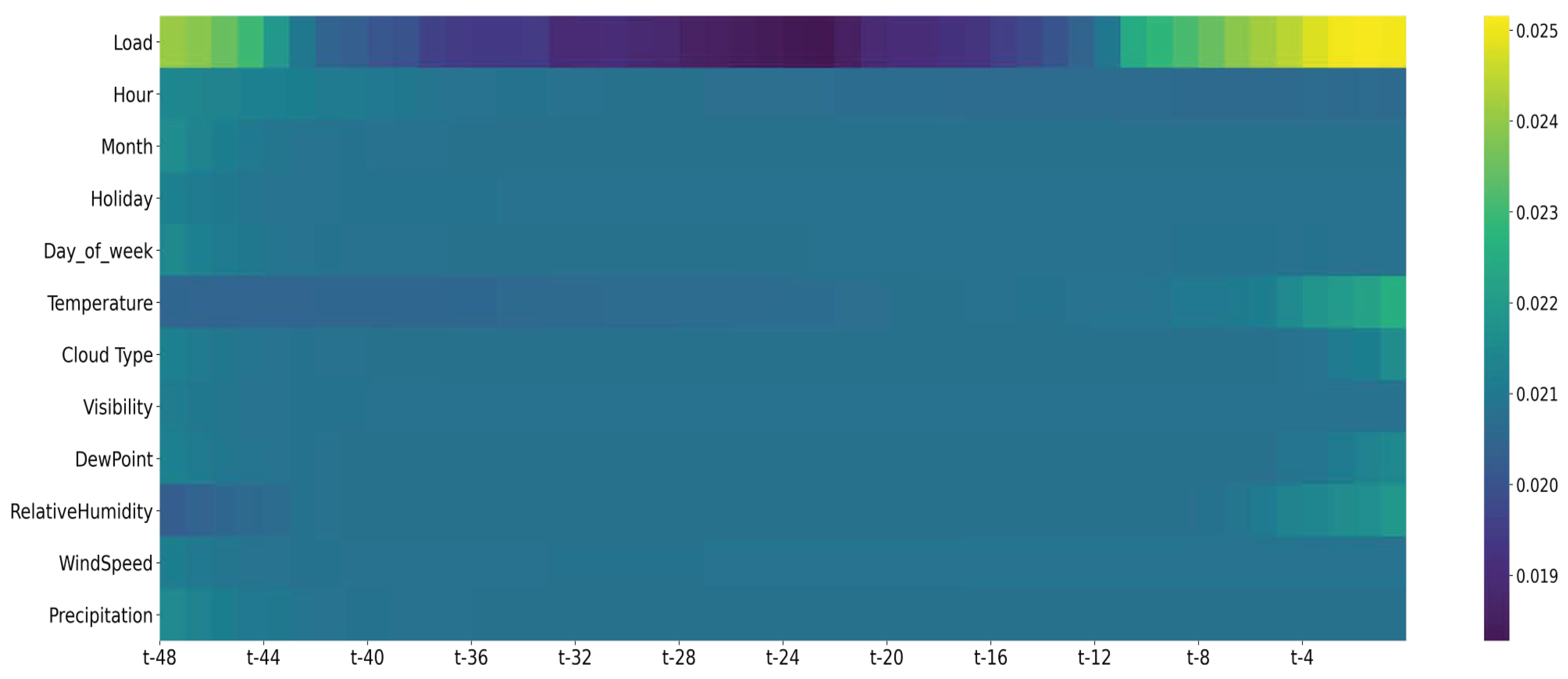
To show the difference in variable importance between different times of the day, we visualize the variable importance for 48 forecasting time steps in Figure 5, where yellow indicates a high-importance variable and blue indicates less influential variable. It can be seen that the history load is the most important at each moment. At the peak time, the effect of the history load becomes larger. During the trough period of electricity consumption, the influence of temperature and hour becomes greater. During peak hours, load consumption is more dependent on consumer behavior, so the importance of load consumption at the previous moments is more prominent. During off-peak hours, people mainly sleep or go out to work. Residential electricity consumption mainly depends on the appliances that must be operated, and the pattern is relatively fixed, and the importance of time-related external factors becomes greater.

4.6. Interpretability Analysis on Temporal Importance

Next, we analyzed the variable-wise temporal importance of the mixture attention mechanism in load forecasting. Figure 6 shows the variable-wise temporal importance results calculated by Equation (16). The rows of the matrix represent the past time steps of the predicted point, and the columns represent the input variables. It can be seen that the importance of the load changed dramatically over time. The load in the last few hours contributed the most to the prediction. This is because the power consumption has a significant lag effect. At the same time, the load at the same moment of the previous day also has a great influence on the prediction. This is related to the periodicity of residential electricity consumption behavior. Changes in temperature also have a greater influence on the load prediction. The temporal importance of temperature increases gradually and the lag effect of temperature is not as large as the load. These show that our model can capture the dynamic changes in different features. The mixture attention mechanism indeed learns useful information for load forecasting, which is consistent with domain knowledge.

5. Conclusions

Due to the flexibility of model development and the availability of fine-grained smart-meter data, the application of deep-learning technology in residential load forecasting has gradually increased. Despite the powerful representational power of deep learning, the complexity of the model reduces interpretability. In this paper, we proposed an interpretable deep-learning method for residential load forecasting, which focuses on mitigating black-box characteristic while improving accuracy. We extended traditional one-step point forecasting to multi-step probabilistic forecasting by employing an encoder–decoder architecture and pinball loss function. The mixture attention mechanism used in each prediction time step can capture different temporal dynamics in a multivariate sequence, which not only improves the prediction performance, but also makes the model inherently interpretable. The experimental results on the real-world data set show that the proposed method has good prediction performance and provides two valuable interpretability aspects: (i) global variable importance and variable importance at different time steps, and (ii) the variable-wise temporal importance. These insights into variable importance and temporal importance reveal the underlying mechanism by which the model works, helping users understand patterns and relationships in the data. They are important for the practical deployment of residential load forecasting models. In addition, by detecting whether these interpretations conflict with the actual electricity load-variation law, it can help decision makers judge the reliability of forecasting results. Finally, these explanations can further help model developers to further improve prediction performance by feature engineering.

The main goal of this work is to train a well-performing interpretable deep-learning prediction model of residential load. A centralized learning approach was used to train a general model, where a large amount of load data was collected by smart meters in different households and shared in a server. However, there are potential privacy leakage issues during communication transmission, as the model can easily infer the living habits of customers, even with the type and usage time of household appliances based on fine-grained load data. Subsequent research should consider combining federated learning [34] to achieve privacy protection. On the other hand, the algorithm complexity is inevitably increased due to the introduction of MV-LSTM. Future methods need to be proposed to compress models, such as feature selection, model distillation, for deployment in home IoT devices with limited computational requirements.