Embedding Soft Thresholding Function into Deep Learning Models for Noisy Radar Emitter Signal Recognition

Abstract

Radar emitter signal recognition under noisy background is one of the focus areas in research on radar signal processing. In this study, the soft thresholding function is embedded into deep learning network models as a novel nonlinear activation function, achieving advanced radar emitter signal recognition results. Specifically, an embedded sub-network is used to learn the threshold of soft thresholding function according to the input feature, which results in each input feature having its own independent nonlinear activation function. Compared with conventional activation functions, the soft thresholding function is characterized by flexible nonlinear conversion and the ability to obtain more discriminative features. By this way, the noise features can be flexibly filtered while retaining signal features, thus improving recognition accuracy. Under the condition of Gaussian and Laplacian noise with signal-to-noise ratio of −8 dB to −2 dB, experimental results show that the overall average accuracy of soft thresholding function reached 88.55%, which was 11.82%, 8.12%, 2.16%, and 1.46% higher than those of Sigmoid, PReLU, ReLU, ELU, and SELU, respectively.

1. Introduction

Accurate radar emitter signal recognition is a critical criterion for determining carriers, objectives, functions, and threat levels of radars [1,2,3]. Practical radar signals, however, tend to be mixed with noise. Therefore, the recognition accuracy of radar emitter signals under a low signal-to-noise ratio (SNR) has been a major research topic in the field of radar signal processing. Early radar emitter signal recognition was mainly achieved by feature matching methods, including the grey correlation analysis [4,5], template matching [6,7], fuzzy matching [8], and attribute measurement [9,10] methods. However, with the continuous development of radar technology, the electromagnetic environment becomes increasingly complex and variable. Moreover, because the feature matching method relies heavily on a priori knowledge, it has drawbacks such as low error tolerance, poor robustness, and complex feature extraction, which prevent it from meeting practical requirements. The rapid development of artificial intelligence techniques has promoted their application to solve the problem of radar emitter signal recognition. Most reported methods are based on time–frequency variation signals in combination with deep learning technology. For instance, signal classification and recognition were achieved on the basis of time–frequency transformation and convolutional neural networks [11,12]. Time–frequency images of signals were obtained by short-time Fourier transform and recognized by deep learning methods [13,14,15]. Based on the deep Q-learning network (DQN), Qu et al. [16] used the time–frequency graph extracted from the Cohen class for signal recognition. However, conversion of the time domain to the time–frequency domain is not only time- and computation-intensive, but also generates excessive noise when the SNR is too low. As a result, the feature discrimination of learning is insufficient and the recognition performance is adversely affected. Meanwhile, most studies adopt conventional deep learning methods, using conventional nonlinear activation functions, with few improvements to the deep learning models. This study proposes a soft thresholding function (SofT), which is a nonlinear activation function that is suitable for radar emitter signal recognition under a low SNR. Furthermore, a novel network model is established by implementing SofT in deep learning methods. The proposed network model does not require time–frequency transformation but directly uses the original one-dimensional (1D) signal as the input. The model then flexibly filters noise according to the input while retaining signal features to improve the recognition accuracy.

2. Methodology

This section introduces the concept of SofT and the design of the SofT module, which is eventually embedded in deep learning methods to improve the recognition accuracy of noisy radar emitter signals.

2.1. Soft Thresholding Function

SofT is a key parameter in wavelet denoising [17]. In the conventional wavelet denoising algorithm, the noise is transformed into a domain near zero, and SofT then removes the features near zero for denoising. 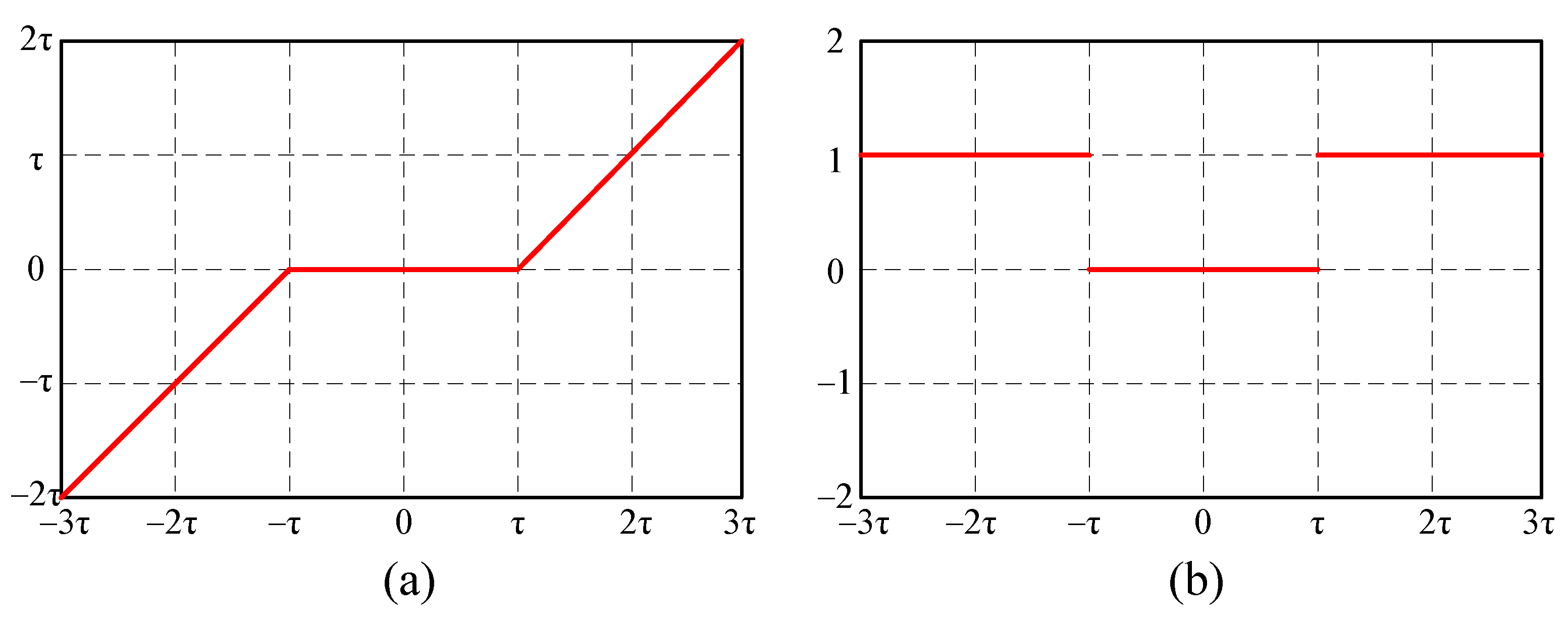In the denoising process, the choice of the wavelet basis function and the number of decomposition layers as well as the threshold selection rule are the key factors affecting the final denoising effect [18]. Determining these parameters requires considerable relevant knowledge and experience, and is therefore often a difficult task. Deep learning methods can automatically learn the weights of features. The combination of SofT and deep learning methods can improve the recognition accuracy while avoiding the complex denoising parameter design. SofT can be described as:

$$y=\left\{\begin{array}{cc}x-\tau & x>\tau \\ 0& -\tau \le x\le \tau \\ x+\tau & x<-\tau \end{array}\right.$$

(1)

where x and y are input and output features, respectively, and $\tau$ is the positive threshold. According to Equation (1), SofT deletes the feature values inside the interval and retains those outside the interval. Figure 1a shows SofT. The partial derivatives of SofT with respect to can be described as:

$$\frac{\partial y}{\partial x}=\left\{\begin{array}{cc}1& x>\tau \\ 0& -\tau \le x\le \tau \\ 1& x>\tau \end{array}\right.$$

(2)

According to Equation (2), the partial derivative of SofT is either 1 or 0, as shown in Figure 1b, which avoids the gradient vanishing problem.

2.2. Soft Thresholding Module

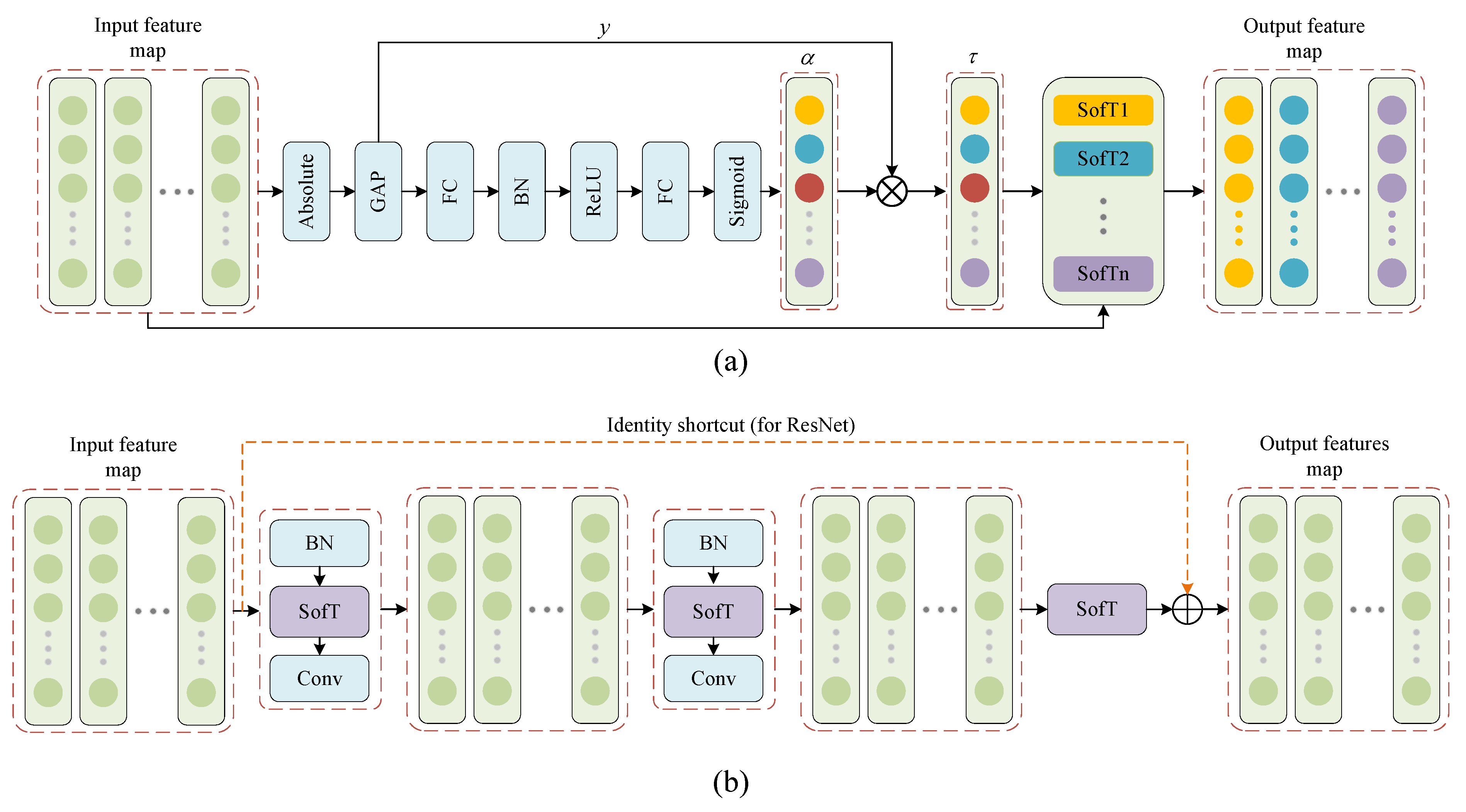
The SofT module uses a sub-network to learn a suitable threshold based on the input features. Therefore, each input feature would have its own independent SofT activation function, which can flexibly filter the noise features while retaining the signal features. The same input and output dimensions are maintained, so it can be easily embedded into the deep learning model. The structure is shown in Figure 2.

As shown in Figure 2a, the SofT module can automatically learn the appropriate value of $\tau$. More specifically, the input feature map is first calculated for absolute values and global averages, which are designed to ensure that the threshold $\tau$ is positive while avoiding the shift variation problem during training. The expression is as follows:

$$y_c=GAP\left(abs\left(x\right)\right)=\underset{i,j}{average}\left(\left|x_{i,j,c}\right|\right)$$

(3)

where y is a 1D vector, c is the index of the channel, x is the input feature map, and $i,j$ are the width and height of the input feature map, respectively. Subsequent to two fully connected layers, the scale parameter can be obtained by:

$${\alpha }_c=sigmoid\left(z\right)=\frac{1}{1+e^{-z_c}}$$

(4)

where z is the output of the fully connected layer. Finally, Equations (3) and (4) are multiplied as shown Equation (5) to obtain the threshold $\tau$ of the input feature:

$${\tau }_c={\alpha }_c·y_c={\alpha }_c·\underset{i,j}{average}\left|x_{i,j,c}\right|$$

(5)

Equation (5) indicates that different channels of the feature map may have different thresholds. This allows more flexibility of the model to retain signal features while removing noise features.

Figure 2b shows a residual building unit (RBU) of the residual network (ResNet), where the conventional activation function ReLU is replaced by SofT. In fact, since the input dimension is the same as the output, the SofT can be easily embedded in any other models in addition to the RBU. Figure 2b comprises two batch normalization (BN), three SofT activation functions, two 1D convolutional layers, and one identity shortcut.

BN is a technique of normalized input feature to reduce the training difficulty and avoid the internal covariant shift problem, which is shown as follows:

$$\mu =\frac{1}{N_{batch}}\sum _{n=1}^{N_{batch}}{x}_n$$

(6)

$${\sigma }^2=\frac{1}{N_{batch}}\sum _{n=1}^{N_{batch}}{(x_n-\mu )}^2$$

(7)

$${\widehat{x}}_n=\frac{(x_n-\mu )}{\sqrt{{\sigma }^2+\epsilon }}$$

(8)

$$y_n=\gamma {\widehat{x}}_n+\beta$$

(9)

Since the radar emitter signal is a one-dimensional sequence, the deep learning models used in this paper all use one-dimensional convolution. Compared with two-dimensional convolution, one-dimensional convolution requires fewer parameters and can extract features directly from the one-dimensional signal while reducing computational resources. The convolution process is defined as follows:

$$y_j=\sum _{i=C}{k}_{ij}\ast x_i+b_j$$

(10)

where $y_j$ represents the jth channel of the output feature map. k is the convolutional kernel, b is the bias, and C is the number of input channels.

3. Experimental and Results

To verify the effectiveness of SofT, five typical activation functions are compared, as shown in

Table 1. Typical activation functions.

Activation Function	Expression
Sigmoid	$y=\frac{1}{1+e^{-x}}$
PReLU	$y=\left\{\begin{array}{cc}x& x\ge 0\\ \alpha x& x<0\end{array}\right.$
ReLU	$y=\left\{\begin{array}{cc}x& x\ge 0\\ 0& x<0\end{array}\right.$
ELU	$y=\left\{\begin{array}{cc}x& x\ge 0\\ \alpha (e^x-1)& x<0\end{array}\right.$
SELU	$y=\lambda \left\{\begin{array}{cc}x& x\ge 0\\ \alpha (e^x-1)& x<0\end{array}\right.$

.

The sigmoid is one of the most common activation functions. It was first used in the LeNet network [19] and achieved the recognition of handwritten digits. The rectified linear unit (ReLU) [20] is also a mainstream activation function, which was applied to the AlexNet network [21] and achieved the state-of-the-art recognition result in the ImageNet LSVRC-2010 contest. ReLU can avoid the gradient disappearance problem and speed up the training process; however, it sets the negative part of the input to zeros, which may lead to the dead relu problem. In contrast, there is a learnable parameter $\alpha$ in PReLU [22], which has a small slope compared to ReLU in the negative region. Thus, the dead relu problem can be avoided in PReLU. However, the parameter $\alpha$ will be fixed after training, resulting in the accuracy of radar emitter recognition is not necessarily better than ReLU. The exponential linear unit (ELU) [23] can also retain negative values of inputs, and make the mean value of output features closer to 0, achieving similar effect as BN but with lower computational complexity. 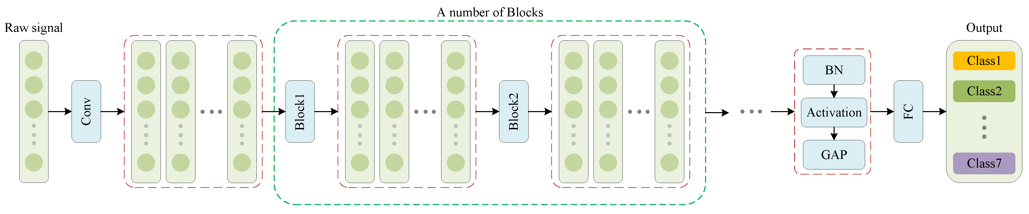The scaled exponential linear unit (SELU) [24] is self-normalizing, which is robust to noise and can also speed up model convergence. In order to verify the effectiveness of SofT, the above five activation functions are embedded into the same network model structure as shown in Figure 3.

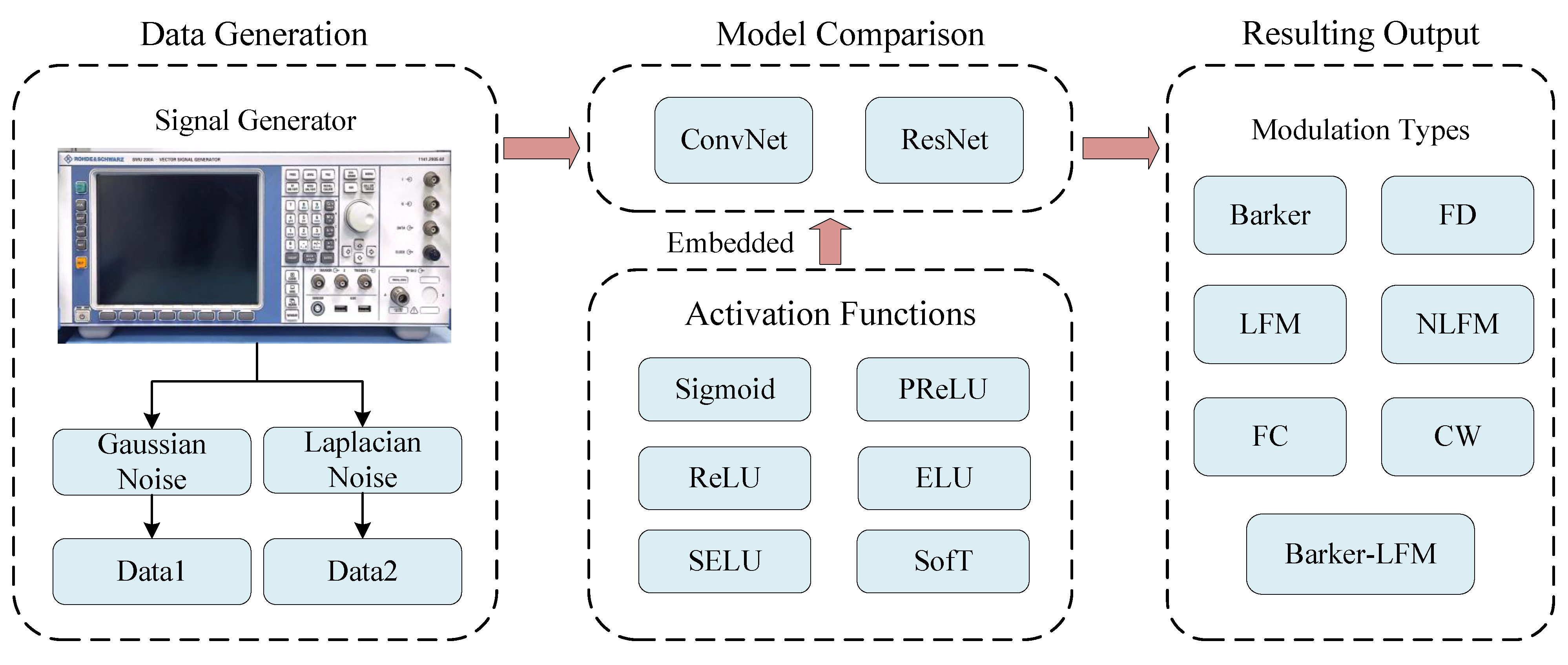
The structure of blocks in Figure 3 are the same as Figure 2b, but SofT will be replaced by each of the five activation functions mentioned above. If the block contains identity shortcuts, the model is ResNet; otherwise, it is ConvNet. The block diagram of this experiment is shown in Figure 4. Firstly, the SMU200A was used to simulate the radar emitter signals, and then two datasets representing different environmental conditions were constructed by adding Gaussian noise and Laplacian noise, respectively. Next, we constructed two models, ConvNet and ResNet, and embedded Sigmoid, PReLU, ReLU, ELU, SELU, and SofT as activation functions into the networks, respectively, to recognize the two kinds of datasets generated. Lastly, different modulation types of signals were output by neural networks.

3.1. Dataset

Seven representative modulation types of radar signals were generated: the Barker code (Baker), the Barker code linear frequency modulation hybrid modulation signal (Baker-LFM), the frequency-coded signal (FC), the continuous wave (CW), the frequency diversity signal (FD), the linear frequency modulation signal (LFM), and the nonlinear frequency modulation signal (LFM). All the radar emitter signal data contain only one pulse, with a data length of 512, and it is worth mentioning that the recognition task of such short single-pulse data is more challenging. The specific signal parameters of the signals are shown in

Table 2. Specific parameters of seven modulation type signals.

Signal Type	Carrier Frequency	Parameter
Barker	10~30 MHz	13-bit Barker code width of each symbol is 1/13 $\mathsf{\mu }$s
Barker-LFM	10~30 MHz	Frequency bandwidth: 100 to 200 MHz 13-bit Barker code width of each symbol is 1/13 $\mathsf{\mu }$s
FC	10~20 MHz 100~200 MHz	13-bit random code width of each symbol is 1/13 $\mathsf{\mu }$s
FD	10~20 MHz 50~60 MHz 90~100 MHz	None
LFM	20~30 MHz	Frequency bandwidth: 50 to 200 MHz 1/2 up frequency modulation 1/2 down frequency modulation
NLFM	20~30 MHz	Frequency bandwidth: 50 to 200 MHz Modulation: quadratic 1/2 up frequency modulation 1/2 down frequency modulation
CW	10~30 MHz	None

The dataset can always be downloaded from https://osf.io/mfa96/ (accessed on 25 January 2022).

.

To verify the effectiveness of SofT, two types of representative noise were added into the radar signals, namely Gaussian noise and Laplacian noise. Gaussian noise has strong randomness in communication channel testing and modeling, and it can seriously disrupt the time domain signal waveform and cover useful information, making signal recognition difficult. Laplacian noise is a non-Gaussian noise. In the actual communication environment, there often exists noise for which the Gaussian noise model cannot be applied, such as impulse noise and co-channel interference. Therefore, it is necessary to use Laplacian noise as non-Gaussian noise for modeling. The SNR range of the Gaussian and Laplacian noise was set from $-8$ dB to $-2$ dB, with an interval of 2 dB, for a total of 4 SNRs. For each noise type, $7\times 4\times 300=8400$ samples were generated, which were randomly divided into training and testing sets in a 2:1 ratio.

3.2. Hyperparameter Setting

Two neural networks, ConvNet and ResNet, were used to compare the performance of different activation functions for radar emitter signal recognition. Furthermore, the number of Blocks was taken as 6, 9, and 12 to test the effect of model depth on performance. The training iterations were 160, the batch size was set to 128, and the initial learning rate was set to 0.1. The learning rate was decayed by a factor of 10 every 40 iterations until the number of iterations was 120, and then was decayed twice in the last 40 iterations. To reduce the randomness, the experiments were repeated 10 times with the same hyperparameter settings, and the mean and variance of the testing accuracy were obtained.

3.3. Experimental Results

The detailed recognition results for different network depths are shown in

Table 3. The average accuracy of the testing set, where M is the number of ResBlocks or ConvBlocks (i.e., ConvBlocks without identity shortcuts) (%).

M	Method	Gauss				Laplace
		$-8$ dB	$-6$ dB	$-4$ dB	$-2$ dB	$-8$ dB	$-6$ dB	$-4$ dB	$-2$ dB
6	ConvNet-Sigmoid	59.34 ± 5.90	74.91 ± 7.35	85.89 ± 4.98	84.60 ± 3.27	67.86 ± 11.98	75.63 ± 9.79	82.14 ± 5.14	85.57 ± 3.01
	ConvNet-PReLU	66.43 ± 1.33	75.54 ± 2.21	86.29 ± 1.35	86.20 ± 1.93	68.54 ± 2.18	78.31 ± 2.73	83.34 ± 1.92	88.34 ± 2.98
	ConvNet-ReLU	70.83 ± 1.61	82.11 ± 2.18	88.20 ± 2.05	91.46 ± 1.19	78.26 ± 3.27	87.09 ± 3.18	91.34 ± 2.11	94.00 ± 1.66
	ConvNet-ELU	73.80 ± 1.78	84.31 ± 0.70	90.26 ± 0.38	92.66 ± 0.67	80.11 ± 1.43	90.14 ± 0.85	92.94 ± 0.95	95.40 ± 0.34
	ConvNet-SELU	73.34 ± 1.78	84.94 ± 0.54	91.49 ± 0.79	93.63 ± 0.75	82.80 ± 0.95	90.23 ± 1.23	94.00 ± 0.74	95.74 ± 0.31
	ConvNet-SofT	75.51 ± 2.98	85.31 ± 4.34	91.84 ± 2.03	94.03 ± 3.41	83.91 ± 2.23	91.09 ± 1.71	94.57 ± 1.82	96.60 ± 1.58
	ResNet-Sigmoid	66.26 ± 1.09	78.89 ± 2.46	86.43 ± 1.91	89.74 ± 1.56	76.89 ± 4.73	84.46 ± 3.27	90.71 ± 2.04	92.94 ± 1.76
	ResNet-PReLU	70.14 ± 1.39	80.94 ± 0.73	87.80 ± 1.42	91.06 ± 1.32	77.17 ± 2.05	84.69 ± 1.67	89.66 ± 0.87	92.89 ± 0.70
	ResNet-ReLU	71.51 ± 1.46	81.89 ± 1.27	88.34 ± 1.42	91.60 ± 2.00	79.37 ± 2.35	87.37 ± 2.25	91.74 ± 0.57	94.66 ± 1.15
	ResNet-ELU	72.46 ± 0.78	85.51 ± 0.51	91.86 ± 0.38	94.51 ± 1.16	81.31 ± 2.60	89.46 ± 1.51	94.00 ± 0.47	95.77 ± 0.82
	ResNet-SELU	72.63 ± 0.42	83.69 ± 2.22	90.89 ± 1.53	93.86 ± 1.37	82.49 ± 1.69	90.06 ± 0.72	94.26 ± 1.11	95.97 ± 0.44
	ResNet-SofT	77.17 ± 1.90	87.49 ± 1.56	92.89 ± 0.80	95.31 ± 1.47	83.09 ± 1.71	90.60 ± 0.36	94.40 ± 1.42	96.37 ± 1.24
9	ConvNet-Sigmoid	55.29 ± 11.79	63.63 ± 16.78	69.60 ± 19.61	73.06 ± 20.21	65.80 ± 19.47	73.54 ± 20.31	81.40 ± 20.77	85.17 ± 16.28
	ConvNet-PReLU	63.69 ± 3.01	71.34 ± 2.88	77.37 ± 2.86	82.00 ± 3.40	66.34 ± 1.86	75.26 ± 2.50	82.23 ± 2.97	86.11 ± 1.84
	ConvNet-ReLU	66.11 ± 2.39	76.60 ± 5.05	83.34 ± 4.11	86.66 ± 3.96	76.11 ± 3.85	85.17 ± 2.69	89.97 ± 2.55	92.06 ± 2.66
	ConvNet-ELU	69.36 ± 8.68	80.34 ± 9.96	84.66 ± 12.78	87.80 ± 13.65	79.86 ± 2.70	86.91 ± 3.81	92.34 ± 3.49	93.94 ± 2.75
	ConvNet-SELU	69.69 ± 5.05	80.51 ± 7.53	86.71 ± 7.69	89.60 ± 7.12	80.69 ± 2.17	89.20 ± 0.94	92.46 ± 0.31	94.77 ± 0.88
	ConvNet-SofT	70.63 ± 2.82	82.63 ± 2.70	89.29 ± 1.28	92.69 ± 2.35	85.31 ± 10.74	91.54 ± 7.92	93.60 ± 6.86	95.40 ± 5.08
	ResNet-Sigmoid	67.06 ± 1.23	79.83 ± 2.81	86.51 ± 3.42	89.86 ± 2.45	77.37 ± 2.05	85.86 ± 1.25	91.71 ± 1.08	94.03 ± 0.50
	ResNet-PReLU	72.34 ± 2.34	81.69 ± 1.37	87.54 ± 1.26	91.69 ± 0.51	79.94 ± 2.36	86.57 ± 2.15	90.29 ± 2.10	95.03 ± 1.30
	ResNet-ReLU	72.57 ± 1.76	83.71 ± 1.26	90.06 ± 1.23	93.00 ± 1.95	80.11 ± 1.72	88.20 ± 1.25	92.77 ± 0.93	95.23 ± 1.10
	ResNet-ELU	73.89 ± 2.12	86.54 ± 1.62	92.29 ± 1.32	94.51 ± 0.74	82.86 ± 2.22	90.09 ± 0.89	94.34 ± 1.43	95.50 ± 1.34
	ResNet-SELU	74.11 ± 1.99	86.71 ± 1.24	92.29 ± 1.47	94.80 ± 1.39	83.54 ± 1.30	90.51 ± 2.20	94.91 ± 0.50	95.74 ± 0.87
	ResNet-SofT	76.74 ± 1.66	87.23 ± 1.29	93.46 ± 1.32	95.71 ± 0.85	84.06 ± 2.58	91.49 ± 1.44	95.29 ± 1.12	96.63 ± 0.44
12	ConvNet-Sigmoid	51.77 ± 9.88	58.43 ± 17.56	63.69 ± 19.99	66.00 ± 21.94	55.40 ± 25.28	62.17 ± 30.24	68.43 ± 31.76	72.06 ± 31.06
	ConvNet-PReLU	61.03 ± 4.37	69.77 ± 3.58	77.89 ± 4.18	83.29 ± 3.72	62.31 ± 2.62	71.23 ± 2.74	77.40 ± 2.37	80.91 ± 3.19
	ConvNet-ReLU	63.86 ± 5.46	72.63 ± 6.30	78.60 ± 7.37	84.46 ± 6.83	68.60 ± 6.08	76.43 ± 8.77	82.71 ± 6.88	87.29 ± 5.97
	ConvNet-ELU	64.66 ± 3.49	75.14 ± 2.39	82.60 ± 2.05	89.57 ± 3.25	73.86 ± 5.89	82.29 ± 5.11	89.11 ± 3.79	91.57 ± 2.59
	ConvNet-SELU	65.17 ± 7.29	77.40 ± 8.41	85.26 ± 5.57	89.74 ± 3.78	77.09 ± 4.74	84.54 ± 3.05	89.20 ± 3.72	91.80 ± 3.28
	ConvNet-SofT	68.31 ± 3.82	80.94 ± 3.03	87.26 ± 3.70	90.11 ± 3.16	78.09 ± 10.96	86.80 ± 8.99	90.74 ± 8.19	92.71 ± 6.27
	ResNet-Sigmoid	65.20 ± 2.78	79.69 ± 2.68	87.69 ± 2.26	91.03 ± 1.25	76.51 ± 3.67	84.66 ± 3.55	86.09 ± 1.62	92.17 ± 1.40
	ResNet-PReLU	72.37 ± 1.70	80.49 ± 1.96	87.74 ± 1.79	91.31 ± 1.21	77.06 ± 2.47	85.69 ± 1.51	88.51 ± 1.00	92.63 ± 1.05
	ResNet-ReLU	72.83 ± 1.03	81.29 ± 1.78	88.09 ± 2.52	92.49 ± 1.81	80.34 ± 1.59	87.86 ± 1.85	92.49 ± 0.42	94.80 ± 0.68
	ResNet-ELU	73.40 ± 1.14	83.86 ± 1.48	91.80 ± 0.85	94.89 ± 0.73	83.11 ± 0.94	90.66 ± 0.90	94.23 ± 0.60	96.06 ± 0.63
	ResNet-SELU	73.91 ± 2.43	85.66 ± 2.04	92.89 ± 0.72	95.06 ± 0.87	84.00 ± 1.51	91.37 ± 0.96	94.37 ± 0.59	96.60 ± 1.19
	ResNet-SofT	77.31 ± 0.98	87.26 ± 1.45	93.23 ± 0.51	95.40 ± 1.17	86.40 ± 1.43	92.14 ± 2.33	95.09 ± 1.19	96.81 ± 1.38

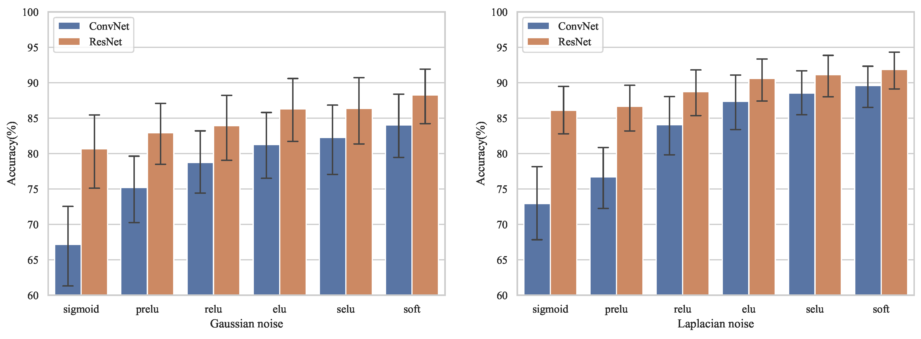
. Herein, ResNet-SofT indicates that ResNet uses SofT as the activation function; other notations are in the similar manner. To compare the effect of different activation functions on the performance of network models more clearly, the overall average recognition accuracy of each activation function is depicted, as shown in Figure 5.

Figure 5 indicates that SofT was superior to conventional activation functions (i.e., Sigmoid, PReLU, ReLU, ELU, and SELU) in terms of recognition accuracy for both Gaussian noise and Laplacian noise.

More specifically, the overall average accuracy of different activation functions is shown as

Table 4. The overall average accuracy of different activation functions (%).

Method	Gaussian Noise	Laplacian Noise
Sigmoid	73.93 ± 7.72	79.52 ± 10.50
PReLU	78.99 ± 2.16	81.69 ± 2.05
ReLU	81.34 ± 2.83	86.42 ± 2.73
ELU	83.78 ± 3.03	88.99 ± 2.00
SELU	84.33 ± 3.08	89.85 ± 1.48
SofT	86.16 ± 2.11	90.95 ± 3.71

. It shows that the overall average accuracy of SofT reached 86.16% for Gaussian noise, which was 12.23%, 7.17%, 4.82%, and 1.83% higher than those of Sigmoid, PReLU, ReLU, ELU, and SELU, respectively. For Laplace noise, the overall average accuracy of SofT reached 90.95%, which was 11.43%, 9.26%, 4.53%, 1.96%, and 1.10% higher than those of Sigmoid, PReLU, ReLU, ELU, and SELU, respectively. Such high recognition rates can be attributed to the fact that the use of SofT as an activation function allows the deep learning model to automatically learn the threshold based on the input, enabling it to flexibly remove noise features while retaining signal features, thus improving radar emitter signal recognition accuracy. Although SELU and ELU are self-normalizing and have some robustness to noise, their parameters are fixed and the network cannot adjust the activation function parameters according to the specific input; therefore, the recognition rate is lower than that of SofT. By contrast, the recognition accuracy of PReLU was unexpectedly lower than that of ReLU. The possible reason for this is that although each channel of the feature graph of PReLU is trained to obtain a multiplicative coefficient during the training process, this coefficient becomes constant during the testing process and cannot be adjusted according to the specific test signal. Therefore, more signal features are preserved while simultaneously introducing more noise, which reduces the discriminative power of high-dimensional features.

In addition, the overall average accuracy of different neural networks is shown as

Table 5. The overall average accuracy of different neural networks (%).

Model	Gaussian Nosie	Laplacian Noise
ConvNet	78.10 ± 5.48	83.28 ± 6.01
ResNet	84.75 ± 1.50	89.20 ± 1.47

. The overall average accuracy of ResNet under Gaussian noise was 84.75%, which is 6.65% higher than that of ConvNet; the overall average accuracy of ResNet under Laplacian noise was 89.20%, which is 5.92% higher than that of ConvNet. This is because embedding SofT as an activation function increases the model complexity and ConvNet faces difficulties in parameter optimization as the number of network layers increases. By contrast, because of the identity shortcuts, ResNet can greatly facilitate the flow of gradients and ease the difficulty of optimization; thus, it has a better recognition performance.

3.4. Feature Analysis

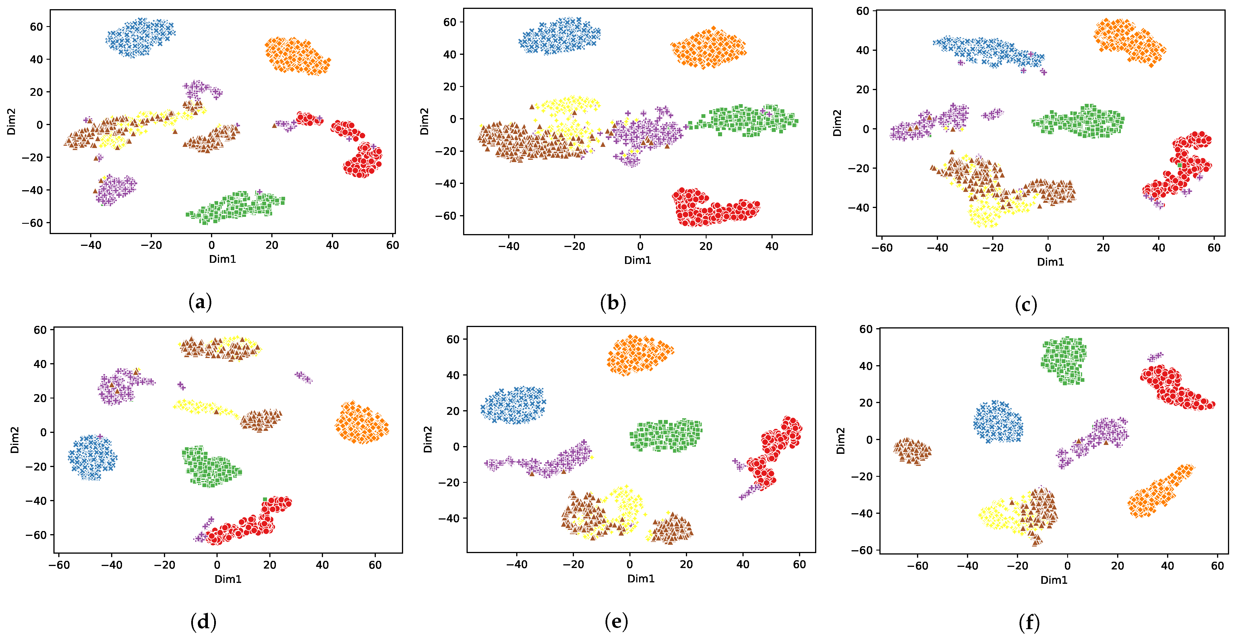
A nonlinear dimensionality reduction method, namely t-distributed stochastic neighbor embedding (t-SNE) [25], was used to analyze the high-dimensional features learned by the network models. Considering space limitation, only the Gaussian noise condition was used to feed the test samples into the trained network models, and the high-dimensional features learned after the last global average pooling layer were extracted and projected into the 2D space using t-SNE for visualization and analysis. As shown in Figure 6 and Figure 7, different colors represent different modulation signals, where red, blue, green, purple, orange, yellow, and brown indicate Barker, Barker-LFM, FC, CW, FD, LFM, and NLFM, respectively. It can be seen that different types of signals were more distinguished in SofT compared to other activation functions under the same deep learning methods. For instance, in ResNet-SofT, the radar emitter signals of the same modulation type were distributed centrally, and the radar emitter signals of different modulation types were separated from each other. By contrast, for ResNet with other conventional activation functions, the 2D feature distributions of different types of signals showed high overlap because the conventional activation function cannot effectively remove noise while retaining discriminative features. Therefore, it is extremely challenging for the conventional deep learning model to distinguish different types of signals under a low SNR condition. As for SofT, the sub-network of the SofT module can learn the appropriate threshold according to the input and effectively remove the noise so that the last layer learned high-dimensional features with strong discrimination.

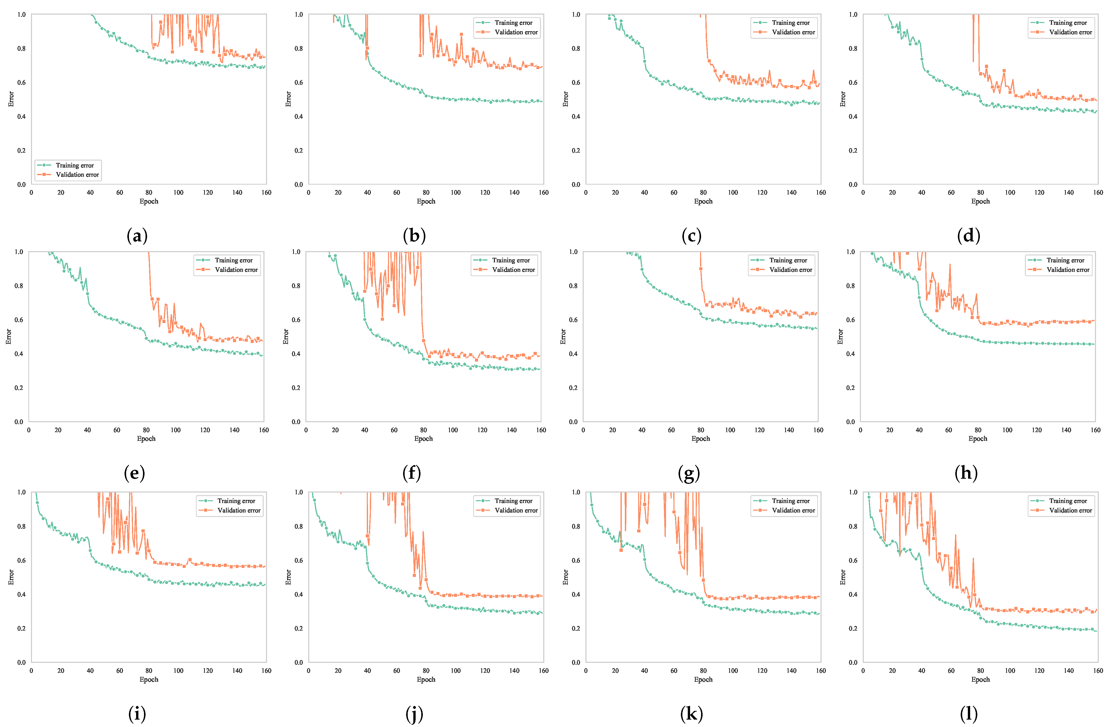
Figure 8 shows the training error and validation error in the training process under the condition of Gaussian noise. As observed, the error curves of all 12 models gradually stabilized after 160 iteration cycles. The smallest training error and validation error were observed for ConvNet-SofT among the six ConvNets and for ResNet-SofT among the six ResNets. Thus, the effectiveness of SofT was validated.

The thresholds learned by the SofT module for different modulation types of signals were compared and analyzed. Specifically, at SNR = $-8$ dB, the seven modulation type signals mentioned in Section 3.1 were input, and the thresholds of the last layer SofT of ConvNet-SofT and ResNet-SofT with nine network layers were output. The results are shown in

Table 6. Thresholds learned by SofT module.

Signal	Threshold
	ConvNet-SofT	ResNet-SofT
Barker	5.530	0.001
Barker-LFM	3.465	1.275
FC	2.893	1.938
CW	2.777	2.640
FD	0.006	0.002
LFM	2.476	2.006
NLFM	4.833	2.123

.

According to Table 6, the learning threshold for different signals in the SofT module is different, which indicates that SofT can learn different thresholds according to the input signal, making it more flexible to remove noise features while retaining signal features in the threshold interval. This also explains why network models with SofT can achieve higher recognition results.

4. Conclusions

To achieve accurate radar emitter signal recognition results, the SofT was embedded into deep learning network models as a novel nonlinear activation function. The SofT module learns different thresholds for different input signals through a sub-network, achieving the purpose of removing noise and improving the feature learning ability of deep learning. The network models with SofT as the activation function do not need to perform dimensional transformation of the inputs but can directly learn discriminative features from the original signal, thus improving the radar emitter signal recognition accuracy.

To verify the effectiveness of the proposed approach, two network models of ConvNet and ResNet with different depths were constructed and tested in two different noisy environments, Gaussian and Laplacian, respectively, and five widely used activation functions, Sigmoid, PReLU, ReLU, ELU, and SELU, were compared. Experimental results revealed that, compared with the methods that use conventional activation functions, the deep learning method based on SofT for the identification of radar emitter signals at a low SNR is significantly superior. More specifically, compared with the overall average recognition rates of Sigmoid, PReLU, ReLU, ELU, and SELU, those of SofT were 12.23%, 7.17%, 4.82%, and 1.83% higher for Gaussian noise and 1.43%, 9.26%, 4.53%, 1.96%, and 1.10% higher for Laplacian noise, respectively. The t-SNE experiments showed that different types of signals are more distinguishable with SofT than with other activation functions, indicating that the learned high-dimensional features are more discriminative.

Therefore, by embedding SofT as a trainable nonlinear activation function into network models, the recognition ability of noisy radar emitter signals can be effectively improved, which is of practical significance for the recognition of radar signals received from actual electromagnetic environments.

5. Discussion

The SofT could be applied to more areas, such as speech recognition in the environment, communication signal recognition and noisy image recognition. However, since the SofT module is trained based on samples, the training set are required to be as extensive as possible, so the next work is to achieve radar emitter signal recognition under small sample conditions.

References

- Petrov, N.; Jordanov, I.; Roe, J. Radar Emitter Signals Recognition and Classification with Feedforward Networks. Procedia Comput. Sci. 2013, 22, 1192–1200. [Google Scholar] [CrossRef] [Green Version]
- Pu, Y.; Liu, T.; Wu, H.; Guo, J. Radar emitter signal recognition based on convolutional neural network and main ridge coordinate transformation of ambiguity function. In Proceedings of the 2021 IEEE 4th Advanced Information Management, Communicates, Electronic and Automation Control Conference (IMCEC), Chongqing, China, 18–20 June 2021. [Google Scholar]
- Richard, W. ELINT: The Interception and Analysis of Radar Signals, 1st ed.; Artech: Norwood, MA, USA, 2006; pp. 6–23. [Google Scholar]
- Huang, Y.; Zhang, H.; Li, L.; Zhou, Y. Radar-Infrared Sensor Track Correlation Algorithm Using Gray Correlative Analysis. In Proceedings of the 2009 International Joint Conference on Artificial Intelligence, Hainan Island, China, 25–26 April 2009. [Google Scholar]
- Xin, G.; You, H.; Xiao, Y. A novel gray model for radar emitter recognition. In Proceedings of the 7th International Conference on Signal Processing, Beijing, China, 31 August–4 September 2004. [Google Scholar]
- Will, C.; Shi, K.; Weigel, R.; Koelpin, A. Advanced template matching algorithm for instantaneous heartbeat detection using continuous wave radar systems. In Proceedings of the First IEEE MTT-S International Microwave Bio Conference (IMBIOC), Gothenburg, Sweden, 15–17 May 2017. [Google Scholar]
- Vignesh, G.J.; Vikranth, S.; Ramanathan, R. A novel fuzzy based approach for multiple target detection in MIMO radar. Procedia Comput. Sci. 2017, 115, 764–770. [Google Scholar] [CrossRef]
- Allroggen, N.; Tronicke, J. Attribute-based analysis of time-lapse ground-penetrating radar data. Geophysics 2016, 81, H1–H8. [Google Scholar] [CrossRef]
- Cahyo, F.A.; Dwitya, R.; Musa, R.H. New approach to detect imminent slope failure by utilising coherence attribute measurement on ground-based slope radar. In Proceedings of the Slope Stability 2020: 2020 International Symposium on Slope Stability in Open Pit Mining and Civil Engineering, Perth, Australia, 12–14 May 2020. [Google Scholar]
- Cheng, H.Z.; Cheng, X.F. A Radar Fault Diagnosis Expert System Based on Improved CBR. Appl. Mech. Mater. 2013, 432, 432–436. [Google Scholar] [CrossRef]
- Zhang, M.; Diao, M.; Guo, L. Convolutional Neural Networks for Automatic Cognitive Radio Waveform Recognition. IEEE Access 2017, 5, 11074–11082. [Google Scholar] [CrossRef]
- Tian, X.; Sun, X.; Yu, X.; Li, X. Modulation Pattern Recognition of Communication Signals Based on Fractional Low-Order Choi-Williams Distribution and Convolutional Neural Network in Impulsive Noise Environment. In Proceedings of the 2019 IEEE 19th International Conference on Communication Technology (ICCT), Xi’an, China, 6–19 October 2019. [Google Scholar]
- Wu, S. Communication modulation recognition algorithm based on STFT mechanism in combination with unsupervised feature-learning network. Peer-to-Peer Netw. Appl. 2019, 12, 1615–1623. [Google Scholar] [CrossRef]
- Liu, H.; Li, L.; Ma, J. Rolling Bearing Fault Diagnosis Based on STFT-Deep Learning and Sound Signals. Shock Vib. 2016, 2016, 6127479. [Google Scholar] [CrossRef] [Green Version]
- Wang, X.; Huang, G.; Zhou, Z.; Gao, J. Radar emitter recognition based on the short time fourier transform and convolutional neural networks. In Proceedings of the 2017 10th International Congress on Image and Signal Processing, BioMedical Engineering and Informatics (CISP-BMEI), Shanghai, China, 14–16 October 2017. [Google Scholar]
- Qu, Z.; Hou, C.; Hou, C.; Wang, W. Radar Signal Intra-Pulse Modulation Recognition Based on Convolutional Neural Network and Deep Q-Learning Network. IEEE Access 2020, 8, 49125–49136. [Google Scholar] [CrossRef]
- Peng, Y.H. De-noising by modified soft-thresholding. In Proceedings of the 2000 IEEE Asia-Pacific Conference on Circuits and Systems, Electronic Communication Systems, Tianjin, China, 4–6 December 2000. [Google Scholar]
- Zhong, J.; Jian, S.; You, C.; Yin, X. Wavelet de-noising method with threshold selection rules based on SNR evaluations. J. Tsinghua Univ. 2014, 54, 259–263. [Google Scholar]
- Lecun, Y.; Jackel, L.; Cortes, C.; Denker, J.; Drucker, H.; Guyon, I.; Muller, U.; Sackinger, E.; Simard, P.; Vapnik, V. Learning Algorithms For Classification: A Comparison On Handwritten Digit Recognition. Neural Netw. Stat. Mech. Perspect. 1995, 261, 2. [Google Scholar]
- Glorot, X.; Bordes, A.; Bengio, Y. Deep sparse rectifier neural networks. In Proceedings of the 14th International Conference on Artificial Intelligence and Statistics, Lauderdale, FL, USA, 11–13 April 2011. [Google Scholar]
- Krizhevsky, A.; Sutskever, I.; Hinton, G.E. ImageNet classification with deep convolutional neural networks. Commun. ACM 2017, 60, 84–90. [Google Scholar] [CrossRef]
- He, K.; Zhang, X.; Ren, S.; Sun, J. Delving Deep into Rectifiers: Surpassing Human-Level Performance on ImageNet Classification. In Proceedings of the 2015 IEEE International Conference on Computer Vision (ICCV), Santiago, Chile, 7–13 December 2015. [Google Scholar]
- Clevert, D.-A.; Unterthiner, T.; Hochreiter, S. Fast and Accurate Deep Network Learning by Exponential Linear Units (ELUs). In Proceedings of the 4th International Conference on Learning Representations (ICLR 2016), San Juan, Puerto Rico, 2–4 May 2016. [Google Scholar]
- Klambauer, G.; Unterthiner, T.; Mayr, A.; Hochreiter, S. Self-normalizing neural networks. In Proceedings of the 31st Conference on Neural Information Processing Systems (NIPS 2017), Long Beach, CA, USA, 4–9 December 2017. [Google Scholar]
- Cieslak, M.C.; Castelfranco, A.M.; Roncalli, V.; Lenz, P.H.; Hartline, D.K. t-Distributed Stochastic Neighbor Embedding (t-SNE): A tool for eco-physiological transcriptomic analysis. Mar. Genom. 2020, 51, 100723. [Google Scholar] [CrossRef]
Figure 1.
(a) Soft thresholding function, (b) soft thresholding function partial derivative.
Figure 2.
(a) Threshold module, (b) residual building unit (RBU).
Figure 3.
Structure of neural network.
Figure 4.
The block diagram of the experiment.
Figure 5.
Overall recognition accuracy of different activation functions.
Figure 6.
Visualization of learned features at the final GAP layer of (a) ConvNet-Sigmoid, (b) ConvNet-PReLU, (c) ConvNet-ReLU, (d) ConvNet-ELU, (e) ConvNet-SELU, and (f) ConvNet-SofT when the number of ConvBlocks equals 9 and SNR equals dB.
Figure 7.
Visualization of learned features at the final GAP layer of (a) ResNet-Sigmoid, (b) ResNet-PReLU, (c) ResNet-ReLU, (d) ResNet-ELU, (e) ResNet-SELU, and (f) ResNet-SofT when the number of ResBlocks equals 9 and SNR equals dB.
Figure 8.
Variation tendency of errors of (a) ConvNet-Sigmoid, (b) ConvNet-PReLU, (c) ConvNet-ReLU, (d) ConvNet-ELU, (e) ConvNet-SELU, (f) ConvNet-SofT, (g) ResNet-Sigmoid, (h) ResNet-PReLU, (i) ResNet-ReLU, (j) ResNet-ELU, (k) ResNet-SELU, and (l) ResNet-SofT when the number of blocks equals 9.