1. Introduction
Deep neural networks (DNN) are computing systems that have now become practically irreplaceable in many areas. It is currently difficult to imagine image/video processing without convolutional neural networks (CNN), and the analysis of time series data without gated recurrent units (GRU) and long short-term memories (LSTM). Thanks to the DNNs, it has become possible to solve many problems that were previously either unsolvable or were solvable, however, at an unsatisfactory level.
However, DNNs are not a magic formula for all problems. There are tasks that do not require large-scale neural architectures and that can be effectively performed by a class of simpler traditional neural networks, having up to five hundred neurons [
1] which, in the context of this paper, are called small/mid-scale networks. Low/high-level robot control [
2,
3,
4,
5,
6,
7], prediction of complex object behaviour [
8,
9,
10], and robot navigation [
11,
12,
13] are examples of tasks that are well-suited for this class of networks.
In order to train ANNs, gradient decent methods are usually applied. Back propagation (BP), with many different variants, is the most popular algorithm that is used for that purpose. However, the drawback of BP is its susceptibility to get stuck in the local optima of an objective function that is optimized during ANN training. In effect, to find a satisfactory neural solution, the algorithm has to be run many times from different starting points which, for complex objective functions with many local optimums, significantly prolongs the training process, and, what is more, it does not give a guarantee of ultimate success.
An alternative solution to the one outlined above is to apply global optimization methods instead of local ones such as BP. Neuro-evolution (NE) seems to be the most popular global optimization approach which, together with BP, is used to train ANNs. However, the problem of NE is the exponentially increasing search space with respect to the number of neurons in the ANN. Even searching for small/mid-scale ANNs involves very large search spaces, including all possible connection weights between the neurons, and the parameters of each neuron: the bias and the transfer function. In turn, complex optimization domains usually need to perform a large number of fitness function evaluations which, in the case of robotic systems, means either huge costs (evaluation on real robots) or a time-consuming process of training the network (evaluation on a complex robot simulation model).
In order to cope with the above problem, the NE methods try to somehow reduce search space, for example, through indirect network representations or some restrictions imposed on possible network architectures. However, all the state-of-the-art NE methods, not only those meant for small/mid-scale networks, are based on the solution, adapted from natural systems, of a one-to-one relation between the network and its genome, i.e., all the information needed to create the network is encoded in a single network representation. As a consequence, simple networks need simple representations, whereas complex networks require complex representations. Meanwhile, the goal of the current paper is to prove that, at least for small/mid-scale networks, an approach that forms neural networks from pieces that evolve in successive evolutionary runs, each of which is responsible for a single piece of the network, not for the entire network, is more efficient than the traditional model of the NE with a one-to-one relation between the network and its genome.
In the paper, an NE method is presented, called Hill Climb Assembler Encoding (HCAE), which is a light version of Hill Climb Modular Assembler Encoding (HCMAE) [
14] and whose target application, unlike its modular counterpart, is the evolution of small/mid-scale neural networks. The main assumption of both HCAE and HCMAE is the gradual growth in the networks and the use of the evolutionary algorithm to generate successive network increments encoded in the form of simple programs that do not grow over time. Instead of more and more complex network representations which are difficult to process effectively, it builds the networks from small pieces that evolve in many consecutive evolutionary runs. The task of each run is to make an improving step in a neural network space. The first run performs in the same way as other traditional NE algorithms. The most effective network from this run is the first step of HCAE. The following runs create the next steps through expanding the network with new neurons and connections or modifying connections that already exist. In contrast to other NE algorithms, HCAE does not process encoded networks but encoded pieces of the networks that are short and simple in effective processing.
HCAE is an improvement of Assembler Encoding (AE) [
15], and Assembler Encoding with Evolvable Operations (AEEO) [
6,
10,
12,
16], i.e., variations of genetic programming (GP) that represent networks in the form of simple programs similar to assembler programs. The major difference between HCAE and its predecessors is the applied model of the evolution. Both AE and AEEO represent the traditional model with the central role of cooperative co-evolutionary GA (CCEGA) [
17,
18], whereas HCAE is in fact a hill climber, whose each step is made by means of CCEGA.
In order to determine how different solutions applied in HCAE affect the results of the algorithm compared with the original solutions used in AE/AEEO, four different variants of HCAE were examined during the tests. The first two variants implemented the new model of the evolution and original mechanisms applied in AE/AEEO, whereas the next two variants implemented improved HCAE mechanisms and the new model of the evolution as well.
After the tests with AE/AEEO, the most effective HCAE variant from the previous experiments was also compared with eight other algorithms. Neuro-Evolution of Augmenting Topologies (NEAT) [
19] and Cooperative Synapse Neuro-Evolution (CoSyNE) [
20] were the first HCAE competitors from outside the AE family, and the reason why they were chosen is that they are regarded as state-of-the-art NE methods with proven effectiveness. Classical Particle Swarm Optimization (PSO) [
21,
22,
23,
24], Levy Flight Particle Swarm Optimization (LFPSO) [
25], modified LFPSO [
26] called PSOLF, and Mantegna Levy Flight, Particle Swarm Optimization, and Neighbourhood Search (LPSONS) [
27] were PSO-based methods applied as the next points of reference for HCAE. The Differential Evolution (DE) [
28,
29,
30] and classic BP algorithm were the last HCAE rivals.
The comparison between HCAE, NEAT, CoSyNE, AE, and AEEO was made on challenging variants of classical identification and control problems, i.e., on the two-spiral problem (TSP) [
31] and inverted-pendulum problem (IPP). In the experiments, the difficulty of both problems was intentionally increased compared with their original variants. TSP is a binary classification problem, and to solve it, feed-forward ANNs (FFANN) are sufficient, whereas the IPP is a control problem that needs recurrent ANNs (RANN). The average complexity of both problems was a deciding factor for why they were selected as a testbed for HCAE and its rivals.
The comparison of HCAE, LFPSO, PSOLF, LPSONS, and BP was made based on the results of experiments reported in [
27]. To this end, thirteen datasets from the UCI machine-learning repository were applied, each of which defines a real classification problem.
In turn, HCAE, DE, and PSO were compared on the trajectory-following problem (TFP). In this case, the task of FFANNs and RANNs was to control an autonomous underwater vehicle (AUV) along a desired trajectory defined spatially and temporally. The TFP is a real problem in underwater robotics, if the coordinated operation of a team of AUVs in time and space is required.
The contributions of the paper are as follows:
The scheme of network evolution applied in HCAE, in which the genome represents a piece of the network, is compared with the traditional model in which the genome represents the entire network.
HCAE is qualitatively evaluated on a number benchmark-classification and control problems.
HCAE is compared with ten other algorithms: AE, AEEO, NEAT, CoSyNE, PSO, LFPSO, LFPSO, LPSONS, DE, BP.
The rest of the paper is organized as follows: section two presents related work, section three details the HCAE, section four reports experiments, section five shows direction of further research, and the final section concludes the paper.
2. Related Work
As already mentioned, the search space of the NE algorithms increases exponentially with every new neuron in the network. For the direct NE methods, which directly and explicitly specify every neuron and connection in the genome, at some point, the search space becomes too large to provide a reasonable chance to design an effective network at all. In order to cope with this problem, in NEAT [
19], which seems to be, currently, the most popular direct algorithm, the genome contains only gens that correspond to existing connections in the network—the connections that do not exist are not represented in the genome. This way, sparsely connected networks can be encoded in the form of short chromosomes, which simplifies the task of NEAT. However, the problem returns for fully or densely connected networks.
To some extent, the above problem can be solved by applying indirect encoding of the networks, in which the genome includes the recipe of how to form the network. The recipe can take different forms, for example, the form of a production rule or a program. By repeatedly using the same rule or a piece of program code in different areas of the evolved neural network, it is possible to generate large-scale networks. In other words, the indirect encoding leads to the compression of the phenotype to a smaller genotype, providing a smaller search space. However, such an approach is only beneficial if the problem solved is modular and has regularities. Otherwise, the indirect representations are just as complex as the direct representations.
In [
32,
33], a developmental approach is presented that is based on production rules that decide how neuron synapses grow and how mother neurons divide. Initially, the mother neurons are placed in 2D space, and then the repeated process of synapse growth and neuron division starts which, after a specified number of iterations, defines the final architecture of the network.
A similar solution is proposed in [
34,
35,
36,
37,
38,
39,
40,
41]. In this case, a grammar is defined including terminals with the network parameters, non-terminals, and the production rules that map non-terminals into terminals or other non-terminals. The networks are represented in the form of encoded starting rules which are run for a number of iterations generating, ultimately, a complete specification of the network.
In order to reduce the dimensionality of fixed topology network representations, the algorithm proposed by [
42] does not work in the weight domain but in the frequency domain. At the phenotypic level, each network is represented as a weight matrix, which, at the genotypic level, is encoded as a matrix of Fourier-transform coefficients, however, without the high-frequency part, which is ignored. To obtain the network, the inverse Fourier transform is applied.
An indirect counterpart of NEAT is HyperNEAT, that is, Hypercube NeuroEvolution of Augmented Topologies [
43]. In the HyperNEAT, networks are produced by other networks called compositional pattern producing networks (CPPNs), which evolve according to NEAT. To generate a network—theoretically, of any size—its neurons are first placed in n-dimensional space, and, then, weights of inter-neuron connections are determined by a single CPPN. To fix a weight between a pair of neurons, the CPPN is supplied with the coordinates of the neurons. An output signal of the CPPN indicates the weight of the connection. Motivated by this approach, a number of variants were proposed to evolve even larger-scale networks [
44,
45,
46,
47]. Moreover, algorithms were also proposed that replace NEAT as the CPPN constructor with genetic programming [
48].
The NE methods based on genetic programming (GP) are a separate class of indirect solutions that represent neural networks in the form of programs. By repeatedly executing the same code in different regions of the network or by cloning neurons/connections, simple programs can represent even large-scale neural networks. In the classical GP, the programs take the form of trees whose nodes include instructions that operate on neurons/connections and control transfer instructions to direct the flow of execution, e.g., sequential/parallel division of a neuron, modification of a weight/bias, jump, and loop [
49,
50,
51,
52].
Gene expression programming (GEP) is a variation of GP in which chromosomes take the form of fixed-length linear strings that, like their tree-structured counterparts, include network-building instructions. The application of GEP to evolve neural networks is presented, among other things, in [
53,
54].
Assembler encoding (AE) [
15] is the next representative of GP. In AE, a network is represented in the form of a linearly organized Assembler Encoding Program (AEP) whose structure is similar to the structure of a simple assembler program. The AEP is composed of two parts, i.e., a part including operations and a part including data. The task of each AEP is to create a Network Definition Matrix (NDM) which includes all the information necessary to produce the network. Unlike instructions of tree-based GP and GEP which work, rather, on the level of individual neurons/connections, each operation of AE can modify even the whole NDM, and, consequently, the network. This way, even a few operations working together within one AEP can form very complex neural structures.
Assembler Encoding with Evolvable Operations (AEEO) [
55] and its modular/ensemble variants [
16,
56] are the successors of AE. Instead of applying hand-made algorithmic operations with evolved parameters, AEEO, like HyperNEAT, uses operations which take the form of simple directly encoded networks, called ANN operations. Just like in the classic variant of the AE, the task of ANN operations, which are run one after the other, is to change the content of the NDM.
Another solution to cope with the problem of large search spaces is the gradual growth in representations and the networks, which is applied, for example, in NEAT [
19], AE [
15], and AEEO [
55]. In this case, the evolution usually starts with light representations and simple networks and increases their complexity in the course of time. The idea is to evolve the networks little by little, and to focus, at each stage of evolution, mainly on genotype/phenotype increments. Initially, small networks and their representations grow if the evolution cannot make progress for a time. Beneficial sub-structures in both genotypes and phenotypes are preserved and gradually expanded with new sub-structures. However, along with the increase in the size of the representations, the complexity of the task of the evolutionary algorithm automatically grows as well. Often, in the late phases of the evolutionary process, the change in the size of chromosomes does not entail any progress in network effectiveness.
There are also NE algorithms that restrict the search space by applying constraints on the network architectures and the evolutionary process. The constraints are usually based on domain knowledge about the problem to be solved. Their task is to focus the search only on allowed network architectures, making the search space for the evolutionary algorithm smaller and its task simpler. In [
1,
57], constraint functions are proposed which directly manipulate neural networks and implement structure, functional, and evolutionary constraints whose task is, for example, to evolve symmetries and repetitive structures, to insert predefined functional units to evolved networks, or to restrict the range of evolutionary operators.
Surrogate model-based optimization [
58,
59] is a solution that does not simplify the task of NE algorithm but alleviates the burden associated with the evaluation of neural solutions scattered over large areas of high-dimensional network space. This is of particular importance in the case of robotic systems whose evaluation requires expansive simulations or real-world experiments. By using surrogate models that mimic the behaviour of the simulation model as closely as possible, being at the same time and computationally cheaper to evaluate, NE algorithms can explore their search spaces more intensely, and thus increase the chance of finding optimal networks.
3. Hill Climb Assembler Encoding
As already mentioned, HCAE is a light variant of HCMAE and it originates from both AE and AEEO. All the algorithms are based on three key components, i.e., a network definition matrix (NDM), which represents the neural networks, assembler encoding program (AEP), which operates on NDM, and evolutionary algorithm, whose task is to produce optimal AEPs, NDMs, and, consequently, the networks. All the three components are described below.
3.1. Network Definition Matrix
To represent a neural network, HCAE, like its predecessors, uses a matrix called network definition matrix (NDM). The matrix includes all the parameters of the network, including the weights of inter-neuron connections, bias, etc. The matrix which contains non-zero elements above and below the diagonal encodes a recurrent neural network (RANN), whereas the matrix with only the content above the diagonal represents a feed-forward network (FFANN) [
14].
3.2. Assembler Encoding Program
In all the AE family, filling up the matrix, and, consequently, constructing an ANN is the task of an assembler encoding program (AEP) which, like an assembler program, consists of a list of operations and a sequence of data. Each operation implements a fixed algorithm and its role is to modify a piece of NDM. The operations are run one after another and their working areas can overlap, which means that modifications made by one operation can be overwritten by other operations which are placed further in the program. AEPs can be homogeneous or heterogeneous in terms of applied operations. In the first case, all operations in AEP are of the same type and they implement the same algorithm whereas, in the second case, AEPs can include operations with different algorithms. The first solution is applied in HCAE and AEEO, whereas the second one in AE [
14].
The way each operation works depends, on the one hand, on its algorithm and, on the other hand, on its parameters. Each operation can be fed with its “private” parameters, linked exclusively to it, or with a list of shared parameters concentrated in the data sequence. Parametrization allows operations with the same algorithm to work in a different manner, for example, to work in different fragments of NDM.
HCAE uses two types of operations, say,
Oper1 and
Oper2.
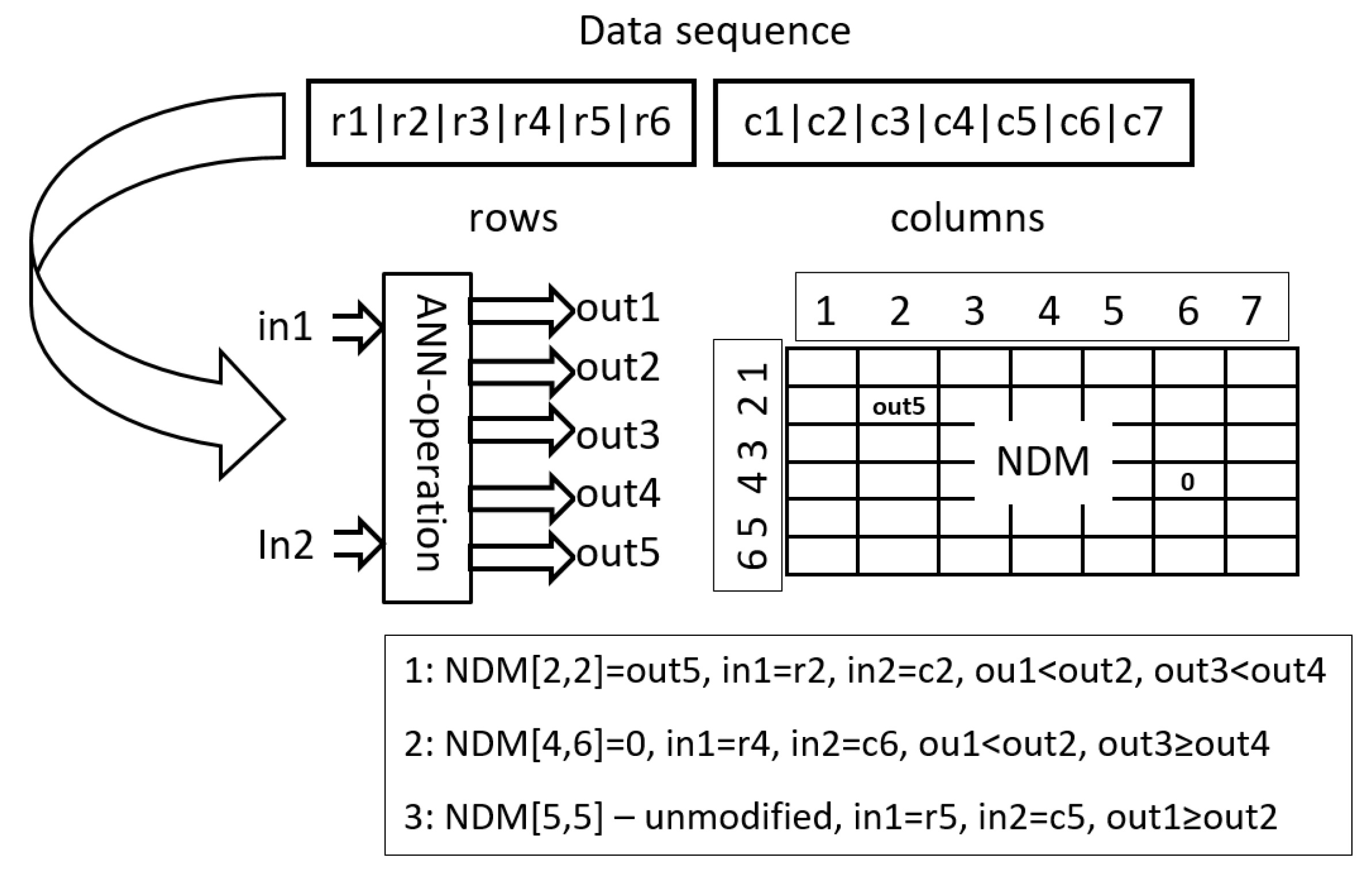
Oper1 is an adaptation of a solution applied in AEEO. It is of a global range, which means that it can modify any element of NDM, and it uses a small feed-forward neural network, say, ANN operation, in the decision-making process. The task of ANN operation is to decide which NDM items are to be updated and how they are to be updated (see
Figure 1). The architecture of each ANN operation is determined by parameters of
Oper1, whereas inputs to the ANN operation are taken from the data sequence of AEP. A pseudo-code of
Oper1 is given in Algorithm 1.
Each ANN operation has two inputs and five outputs. The inputs indicate individual items of NDM. In AEEO, ANN operations are fed with coordinates of items to be modified, that is, with numbers of columns and rows, for example, in order to modify item [], an ANN operation is supplied with i and j. In HCAE, a different approach is used, namely, instead of i, j, ANN operations are fed with data items which correspond to i and j, that is, with row [i] and column [j] (lines (10) and (11) in Algorithm 1). Vectors row and column are filled with appropriate data items (lines (2) and (5) in Algorithm 1).
The outputs of ANN operation decide whether to modify a given item of NDM or to leave it intact—outputs no. 1 and no. 2 (line (13) in Algorithm 1), and then, whether to reset the item or to assign it a new value—outputs no. 3 and no. 4 (line (14) in Algorithm 1), the new value is taken from the fifth output of the ANN operation (line (15) in Algorithm 1). Parameter
M is a scaling parameter.
| Algorithm 1 Pseudo-code of Oper1. |
Input: operation parameters (p), data sequence (d), NDM
Output: NDM
1: for i∈<0..NDM.numberOfRows) do
2: row[i] ← d[i mod d.length];
3: end for
4: for i∈<0..NDM.numberOfColumns) do
5: column[i] ← d[(i+NDM.numberOfRows) mod d.length];
6: end for
7: ANN-oper ← getANN(p);
8: fori∈<0..NDM.numberOfColumns) do
9: for j∈<0..NDM.numberOfRows) do
10: ANN-oper.setIn(1,row[j]);
11: ANN-oper.setIn(2,column[i]);
12: ANN-oper.run();
13: if ANN-oper.getOut(1) <ANN-oper.getOut(2) then
14: if ANN-oper.getOut(3) < ANN-oper.getOut(4) then
15: NDM[j,i] ←M*ANN-oper.getOut(5);
16: else
17: NDM[j,i] ← 0;
18: end if
19: end if
20: end for
21: end for
22: Return NDM |
Like resultant ANNs, ANN operations are also represented in the form of NDMs, say, NDM operations. To generate an NDM operation, and consequently, an ANN operation,
getANN(p) is applied whose pseudo-code is depicted in Algorithm 2. It fills all matrix items with subsequent parameters of
Oper1 divided by a scaling coefficient,
N. If the number of parameters is too small to fill the entire matrix, they are used many times.
| Algorithm 2 Pseudo-code of getANN. |
Input: operation parameters (p)
Output: ANN-operation
1: NDM-operation ← 0;
2: noOfItem← 0;
3: for i∈<0..NDM-operation.numberOfColumns) do
4: for j<i //feed-forward ANN do
5: NDM-operation[j,i] ← p[noOfItemmod p.length]/N;
6: noOfItem++;
7: end for
8: end for
9: Return ANN-operation encoded in NDM-operation. |
Unlike
Oper1,
Oper2 works locally in NDM, and is an adaptation of a solution applied in AE. Pseudo-code of
Oper2 is given in Algorithm 3 and 4. It does not use ANN-operations; instead, it directly fills NDM with values from the data sequence of AEP: where NDM is updated, and which and how many data items are used, are determined by operation parameters. The first parameter indicates the direction according to which NDM is modified, that is, whether it is changed along columns or rows (lines (4) and (10) in Algorithm 3). The second parameter determines the size of holes between NDM updates, that is, the number of zeros that separate consecutive updates (line (3) in Algorithm 4). The next two parameters point out the location in NDM where the operation starts to work, i.e., they indicate the starting row and column (line (1) in Algorithm 4). The fifth parameter determines the size of the altered NDM area, in other words, it indicates how many NDM items are updated (line (1) in Algorithm 4). Additionally, the last, sixth parameter points out location in the sequence of data from where the operation starts to take data items and put them into the NDM (line (2) in Algorithm 3) [
14].
| Algorithm 3 Pseudo-code of Oper2 [14]. |
Input: operation parameters (p), data sequence (d), NDM
Output: NDM
1: filled← 0;
2: where← p[6];
3: holes← 0;
4: if p[1] mod 2 = 0 then
5: for k∈<0..NDM.numberOfColumns) do
6: for j∈<0..NDM.numberOfRows) do
7: NDM[j,k] ← fill(k,j,param,data,filled,where,holes);
8: end for
9: end for
10: else
11: for k∈<0..NDM.numberOfRows) do
12: for j∈<0..NDM.numberOfColumns) do
13: NDM[k,j] ← fill(j,k,p,d,filled,where,holes);
14: end for
15: end for
16: end if
17: Return NDM. |
| Algorithm 4 Pseudo-code of fill () [14]. |
Input: number of column (c), number of row (r), operation parameters (p),
data sequence (d), number of updated items (f),
starting position in data (w), number of holes (h)
Output: new value for NDM item
1: if f < p[5] and c ≥ p[4] andr≥ p[3] then
2: f++;
3: if h = p[2] then
4: h ← 0;
5: w++;
6: Return d[w mod d.length];
7: else
8: h++;
9: Return 0.
10: end if
11: end if |
3.3. Evolutionary Algorithm
The common characteristic of all AE-based algorithms is the use of cooperative co-evolutionary GA (CCEGA) [
17,
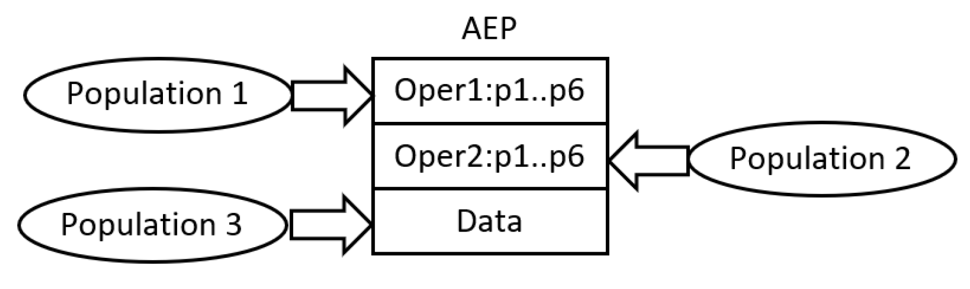
18] to evolve AEPs, that is, to determine the number of operations (AE,AEEO), the type of each operation (AE), the parameters of the operations (all algorithms), the length of the data sequence (AE,AEEO), and its content (all algorithms). As already mentioned, the implementations of operations are predefined. According to CCEGA, each evolved component of AEP evolves in a separate population, that is, an AEP with
n operations and the sequence of data evolves in
populations (see
Figure 2) [
14].
To construct a complete AEP, NDM, and finally, a network, the operations and the data are combined together according to the procedure applied in CCEGA. An individual (for example, an operation) from an evaluated population is linked to the best leader individuals from the remaining populations that evolved in all previous CCEGA iterations. Each population maintains the leader individuals, which are applied as building blocks of all AEPs constructed during the evolutionary process. In order to evaluate newborn individuals, they are combined with the leader individuals from the remaining populations [
14].
Even though all the AE family applies CCEGA to evolve neural networks, HCAE does it in a different way from the remaining AE algorithms. In AE/AEEO, the networks evolve in one potentially infinite loop of CCEGA. Throughout the evolution, AEPs can grow or shrink, that is, they adjust their complexity to the task by changing in size. Each growth or shrinkage entails a change in the number of populations in which AEPs evolve. Unfortunately, such an approach appeared to be ineffective for a greater number of operations/populations. Usually, an increase in the number of operations/populations to three or more does not improve results, which is due to the difficulties in the coordination of a greater number of operations.
In contrast to AE/AEEO, HCAE is a hill climber whose each step is made by CCEGA (see Algorithm 5). A starting point of the algorithm is a blank network represented by a blank NDM (line (1)). Then, the network as well as NDM are improved in subsequent evolutionary runs of CCEGA (line (5)). Each next run works on the best network/NDM found so far by all earlier runs (each AEP works on its own copy of NDM), is interrupted after a specified number of iterations without progress (
MAX_ITER_NO_PROG), and delegates outside, to the HCAE main loop, the best network/NDM that evolved within the run (tempNDM). If this network/NDM is better than those generated by earlier CCEGA runs, a next HCAE step is made—each subsequent network/NDM has to be better than its predecessor (line (7) [
14] ).
| Algorithm 5 Evolution in HCAE [14]. |
Input: CCEGA parameters, for example crossover probability
Output: Neural network
1: NDM ← 0;
2: numberOfIter← 0;
3: fitness← evaluation of NDM;
4: while numberOfIter < maxEval and fitness < acceptedFitnessdo
5: tempNDM ← CCEGA.run(NDM,MAX_ITER_NO_PROG);
6: if tempNDM.fitness > fitness then
7: NDM ← tempNDM;
8: fitness ← tempNDM.fitness;
9: end if
10: numberOfIter ← numberOfIter + 1;
11: end while
12: Return Neural network decoded from NDM. |
In order to avoid AE/AEEO problems with the effective processing of complex AEPs, HCAE uses constant-length programs of a small size. They include, at most, two operations and the sequence of data; the number of operations does not change over time. Such a construction of AEPs affects the structure of CCEGA. In this case, AEPs evolve in two or, at most, three populations; the number of populations is invariable. One population includes sequences of data, i.e., chromosomes data, whereas the remaining populations contain encoded operations, i.e., chromosomes operations. The operations are encoded as integer strings, whereas the data as real-valued vectors, which is a next difference between HCAE and AE/AEEO that apply binary encoding. Both chromosomes operations and chromosomes data are of constant length.
In HCAE, like in AE/AEEO, the evolution in all the populations takes place according to simple canonical genetic algorithm with a tournament selection. The chromosomes undergo two classical genetic operators, i.e., one-point crossover and mutation. The crossover is performed with a constant probability
, whereas the mutation is adjusted to the current state of the evolutionary process. Its probability (
—probability of mutation in data sequences;
—probability of mutation in operations) grows once there is no progress for a time and it decreases once progress is noticed [
14].
The chromosomes data and chromosomes operations are mutated differently, and they are performed according to Equations (
1) and (
2) [
14].
where
d—is a gene in a chromosome-data;
o—is a gene in a chromosome-operation; randU(
)—is a uniformly distributed random real value from the range
; randI(
)—is a uniformly distributed random integer value from the range
;
—is a probability of a mutated gene to be zero.
3.4. Complexity Analysis
Although algorithms no. 1, 2 and 3 present the traditional iterative implementation style, which is due to the ease of analysis of such algorithms, the actual HCAE implementation is parallel. This means that the algorithm can be divided into three parallel blocks executed one after the other, namely: the genetic algorithm (CCEGA + CGA), the AEP program and the evaluation of neural networks. The complexity of the algorithm can therefore be defined as O(O(CCEGA + CGA) + O(AEP) + O(Fitness)). The parallel implementation of the genetic algorithm requires, in principle, three steps, i.e., selection of parent individuals, crossover and mutation, which means that we obtain O(3). In addition, it also requires processors or processor cores, where l is the number of chromosomes in a single CCEGA population, is the number of AEP operations, and n and are the number of genes in chromosome data and chromosomes operations, respectively. The AEP program is executed in steps (O()) and requires a maximum of Z processors/cores, where Z is the number of cells of the NDM matrix. The last block of the algorithm is the evaluation of neural networks, the computational complexity of which depends on the problem being solved. Ignoring the network evaluation, it can be concluded that the algorithm complexity is O(3 + ) and requires processors/cores.
4. Experiments
As already mentioned in the introduction, HCAE was tested on fourteen classification problems and one control problem against eight rival methods. First, HCAE(AE) and HCAE(AEEO) algorithms were tested on the two-spiral problem (TSP) and the inverted-pendulum problems (IPP) against original AE and AEEO. HCAE(AE) and HCAE(AEEO) are algorithms that evolve networks according to the HCAE algorithm depicted in Algorithm 5; however, at the same time, they apply AE and AEEO operations, binary encoding, variable-size chromosomes, and CCEGA mechanisms of adapting size of AEPs to a problem—AEPs can change their size throughout the evolution. The goal of this phase of the experiments was to examine the effectiveness of the new model of evolution applied in HCAE.
In the second stage of the experiments, HCAE(AE) and HCAE(AEEO) competed with HCAE(Oper1) and HCAE(Oper2) with the goal of testing the new operations applied in HCAE. Again, TSP and IPP constituted a testbed for the compared algorithms.
The third phase of the experiments was devoted to the comparison between HCAE, NEAT (C++ implementation of NEAT was taken from [
60]), and CoSyNE (C++ implementation of CoSyNE was taken from [
61]). Only the most effective variant of HCAE took part in the tests. As before, the task of the selected algorithms was to evolve neural solutions to TSP and IPP problems.
Finally, HCAE was also compared with four PSO-based algorithms considered in [
27] and with backpropagation (BP). This time, the algorithms were put to the test on thirteen classification problems defined in the UCI machine-learning repository. The objective of both of the last phases of the experiments was to present HCAE against other algorithms in the field of NE.
4.1. Two-Spiral Problem
TSP, which is a well-known benchmark for binary classification, was selected as a starting problem for HCAE and its rivals. Even though it is not a new problem, its average complexity corresponds to the complexity of problems that can be effectively solved with small/medium-size neural networks and learning algorithms dedicated to such networks.
In TSP, the task is to split into data points that form intertwined spirals which cannot be linearly separated into two classes. The learning set consists of 194 points, 97 for each spiral. To generate the first spiral, the following formulas can be used: , , , . The second spiral can be obtained by the negation of first spiral coordinates, that is, by: .
To solve the above-mentioned problem, feed-forward neural networks with two inputs, two outputs, and maximally thirty-six hidden neurons were applied. The inputs were fed with the coordinates of data points, whereas outputs were responsible for identification, one output for one class. If the output signal of the first output neuron was greater than the output signal of the second output neuron, an input data point was assigned to the first class, otherwise, to the second class. All neurons in the networks used a hyperbolic tangent activation function.
When evolving the networks, the algorithms were allowed to make, maximally, 3,000,000 evaluations. In order to evaluate each evolved neural network, the following fitness function was applied:
where
S—is the number of correct classifications up to the first wrong decision; in the case of a wrong decision, the evaluation process was immediately interrupted;
—is an error in
i-th learning iteration in which the first wrong decision was made; in the learning process two classes were presented alternately to the network, which means that points from the first class even had indexes in the learning set (
i mod
), whereas points from the second class had odd indexes (
i mod
),
and
are outputs of the neural network; the formal definition of
is given below:
The fitness function (3) introduces additional difficulties compared with the original problem defined in [
31]. Originally, in order to evaluate the network, classification results on all training points are used. This corresponds to the situation in which the learning algorithm has complete knowledge of the effectiveness of the network in the whole range of the input space (considered in the learning set). Meanwhile, according to (3), the learning algorithm is forced to rely on partial knowledge. If the network fails at some point, the evaluation process is interrupted with the consequence that the algorithm has only insight into fragmentary capabilities of the evaluated network and its evaluation can be misleading. For example, a network successful in the first
n points will be more fit than a network successful in
m points in total;
, however, in only
k consecutive points from the top of the learning point list,
.
Error (
4) has three options. The first option
drastically reduces the network fitness if
. In the absence of this option, function (
3) would have a deep local maximum for
, at which the algorithm would often get stuck. The other two options are just the sum of the errors on each network output. For the first class, the ideal situation is
,
, while for the second class,
, and
.
4.2. Inverted-Pendulum Problem
In order to assess how HCAE copes with evolving recurrent neural networks (RANN) dedicated for control problems of average complexity, and to compare its performance in this regard with the performance of other algorithms, experiments in the inverted-pendulum problem (IPP) were carried out. Even though the original variant of IPP was defined quite a long time ago [
20], the modified version applied in the experiments is enough to achieve the goal of the research mentioned above.
In this case, the networks deal with a wheeled cart moving on a finite length track and with two poles installed on the cart; one pole is shorter and lighter, whereas the second one is longer and heavier. The task of the networks is to indefinitely balance the poles and to keep the cart within track boundaries. To accomplish the task, the cart has to be pushed left or right with a fixed force. The decision about the direction and the strength of each move is made based on the information about the state of the cart-and-pole system. The complete state vector includes the following parameters: the position of the cart (
x), the velocity of the cart (
), angles of both poles (
,
), and angular velocities of both poles (
,
). To model behaviour of the cart-and-pole system, the following equations are used [
20]:
where
—acceleration of cart;
—acceleration of
ith pole;
F—force put to cart;
M—mass of cart;
—mass of
ith pole;
—half length of
ith pole;
—coefficient of friction of cart on track;
—coefficient of friction of
ith pole’s hinge;
g—gravity.
The state of the cart-and-pole system in subsequent points in time of simulation, i.e., every
t seconds, where
t is a step size, is determined by means of Euler’s method:
To control the cart-and-pole system, the networks were fed with the state parameters scaled to the range . The force F used to control the system was calculated as a product of network output (one output neuron) and value 10. To make the task of the networks more difficult, they had access to only two parameters, i.e., x, and (two input neurons). This means that they had no information about the shorter pole, and they did not know the direction of movement and velocity of the cart and the longer pole. To effectively control the cart-and-pole system, all missing information had to be reconstructed by the networks in the subsequent steps of the simulation.
The above-mentioned setting was not the only impediment the networks had to face. In contrast to the original problem, each network was evaluated four times, each time for other starting conditions, and each single evaluation was interrupted once the cart went off the path or any pole fell down, that is, exceeded a failure angle. In order for the task of the networks to be even harder in relation to the original problem [
20], the failure angels for both poles were decreased to 8 degrees for the longer pole, and 20 degrees for the shorter one. The other experiment settings remained unchanged in relation to [
20] and are given in
Table 1.
The networks applied in the experiments had the following architecture: two inputs, one output, and, maximally, forty hidden units. When evolving the networks, the algorithms were allowed to make, maximally, 30,000 evaluations. In order to evaluate each evolved neural network, the following fitness function was applied:
where
is the duration of
ith simulation that was measured as the number of steps the cart-and-pole system remained controlled. The maximum duration of each single simulation was equal to 10,000 control steps, which means that the maximum fitness that could be achieved was 40,000. The task of function (
13) is simply to obtain a network capable of holding the pendulum up for as long as possible in each of the four simulations.
4.3. Trajectory-Following Problem
In this case, the task of the neural networks was to guide the AUV along a desired trajectory defined spatially and temporally. Given that the AUV trajectory is determined by a set of way points in 2D space (it is assumed that the AUV moves on the horizontal plane without depth control) and each straight segment between two way points has a march velocity (
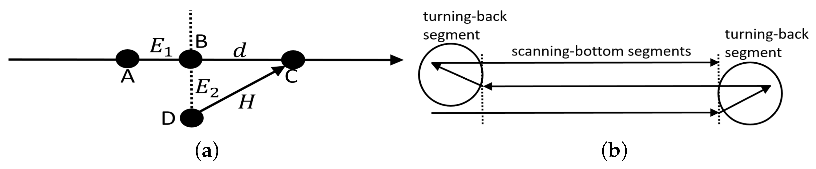
) assigned, at each point in time, it is possible to determine a desirable position of the AUV and two errors in the position, i.e., the position error calculated along the trajectory—
, and the position error perpendicular to the trajectory—
.
indicates the timing error, that is, whether the AUV is late or ahead of time, whereas
corresponds to the distance to the right trajectory—see
Figure 3a.
The neural network controls the vehicle by determining its heading
H and speed
V in such a way as to minimize the errors
and
. The new parameters of the AUV movement are defined every 0.1 s. The heading of the vehicle is determined from point D (see
Figure 3a), where the vehicle is currently located, to point C, which is the local destination of the AUV. To find point C, the neural network determines the distance
d from point B towards the next way point.
Speed V is the sum of the marching speed associated with each straight section of the vehicle route and speed determined by the neural network.
Both FFANN and RANN networks were used during the research. In both cases, the networks were supplied with and errors. The error was positive if the vehicle was late and negative—if it was in a hurry. The error was always positive. FFANN networks had four inputs, two inputs corresponding to errors from the current time moment and two inputs corresponding to errors from the previous time moment. The RANN networks had only two inputs corresponding to the errors that occurred at the current time.
Apart from two output neurons (d and ) and two or four input neurons, both types of networks had 10 hidden neurons. All the neurons had the same activation function—the hyperbolic tangent function.
The tests were carried out in simulation conditions using a kinematic vehicle model implemented in the MOOS-IvP application called uSimMarine [
62]. This model has a number of parameters determining the speed of the vehicle, its manoeuvrability or inertia. The description of the parameters with their values used during the simulation can be found at the end of the paper, in
Appendix B.
During the simulation, the behaviour of the vehicle was also influenced by the low-level control system, whose task was to convert high-level decisions made by the neural network into low-level decisions for the propellers (engine) and rudder of the vehicle. The low-level system consisted of four PID controllers, each with three parameters: P, I, and D, the values of which are given in
Appendix B.
The task of the AUV was to follow a lawn-mower trajectory consisting of eight way points and seven straight segments, i.e., three 100-m long scanning-bottom segments and four turning-back segments—see
Figure 3b. The march speed
along the scanning-bottom segments amounted to 1 m/s, whereas, along the turning–back segments, it amounted to 0.5 m/s.
For the conditions of the experiments to be maximally similar to the real ones, the AUV was subject to a sea current which had random duration, direction and strength. It appeared regularly every 6 s at most, and its maximum duration amounted to 2 s. The direction of the current amounted to 4510, whereas its strength amounted, maximally, to 0.8 m/s.
Each of the evolutionarily formed networks was evaluated
k times, each time with a different influence of the sea current;
= 40. The evaluation of the network was always interrupted (
) if the error
or
exceeded the threshold value equal to 3 m and 2 m, respectively. The following fitness function was used to evaluate the networks:
where
and
are the maximum errors obtained during the entire network-evaluation process, while the AUV was moving along the scanning-bottom segments of the trajectory. Short turning-back segments were not included in the evaluation. In order to obtain the precise trajectory of the vehicle along the entire scanning-bottom segments, function (
14) was oriented to minimize maximum errors. Error
has a greater influence on function (
14), which means that more emphasis is on minimizing the spatial deviation from the trajectory than the temporal deviation.
4.4. Results in the First Phase of Experiments
As already mentioned, the objective of this phase was to evaluate the effectiveness of the new model of evolution applied in HCAE. To this end, original AE and AEEO were compared with HCAE(AE) and HCAE(AEEO) which are variants of AE/AEEO with the HCAE model of evolution.
At the beginning, AE and AEEO were tuned to both testing problems (TSP and IPP), mainly by adjusting the probability of mutation. Other parameters were either manually tailored to the tasks, for example: size of NDM-operation =
neurons in total, one extra column for biases, crossover probability
, size of each population = 100, size of tournament = 3, length of chromosome-data = 80, initial number of operations = 1, length of chromosome-operations = 12 or 6, number of CCEGA iterations without progress followed by a change of AEP size = 100,000 (TSP) or 2500 (IPP), or they were the same as those applied in [
15,
16].
In order to compare the algorithms, each of them were run thirty times. Then, thirty of the most effective networks from all the runs, one network per run, were applied to compare the algorithms. Four criteria were used to measure the performance of each algorithm, i.e., the average, maximum, and minimum fitness, and the total number of successes in the learning process (TSP—all learning data points classified correctly, IPP—the poles successfully balanced in all attempts). The final results of the tests are summarized in
Table 2 and
Table 3.
Both tables clearly show the positive effect of HCAE model of evolution on the performance of AE/AEEO. The greatest increase in efficiency is noticeable when comparing results of HCAE(AE) and AE. A smaller improvement is observed in the case of HCAE(AEEO) and AEEO.
The result proves, at least with regard to evolutionary neural networks and the AE family, that the model in which the evolution is conducted in many separate evolutionary runs and each earlier run produces input data for its successors, when the solutions grow gradually in many subsequent increments, and when the complexity of the genome is replaced with a sequence of simple genomes, outperforms a traditional model in which the complexity of the problem corresponds to the complexity of the genome and the whole problem has to be solved within one evolutionary super run.
Two main factors seem to decide the success of the HCAE model: firstly, the strategy of gradual growth, and secondly, the simplicity of representation. However, as the above results show, the success depends on the interference between subsequent evolutionary runs and between operations inside AEP—the greater the interference, the smaller the success. To put it simply, if operations within one AEP, or AEPs executed one after another, strongly interfere with each other, it is difficult to achieve the effect of gradual growth.
One objective of the HCAE model is to simplify AEPs as much as possible with the task to simplify cooperation between operations derived from different populations. It is simply much easier to match two or three components of a solution together than to do it with, say, five or ten components. In other words, the interference between two or three operations is smaller than the interference between five or ten operations. To make matters worse, the interference can also apply to operations from different evolutionary runs.
However, the interference between operations depends not only on the number of operations in AEP but also on the range of operations, which is different in HCAE(AE) and HCAE(AEEO). In the first case, the operations work locally in a selected region of NDM, whereas in the second case, they are allowed to update each element of NDM. In consequence, operations applied in HCAE(AE) rarely interfere with each other, whereas those used in HCAE(AEEO) do it much more often. This, in turn, means that the strategy “little by little” implemented in HCAE has a greater chance for success in combination with AE than AEEO.
4.5. Results in the Second Phase of Experiments
In this phase, the objective was to evaluate the effectiveness of the remaining solutions applied in HCAE compared with their originals from AE and AEEO. The results of this phase are given in
Table 4 and
Table 5.
As it turned out, new solutions implemented in HCAE(Oper2) appeared to have an advantageous influence on the algorithm performance compared with HCAE(AE). In turn, for those applied in HCAE(Oper1), if they brought any positive effect it is visible only in TSP. In IPP, the results of HCAE(Oper1) and HCAE(AEEO) are roughly at the same level.
The new solutions implemented in HCAE can be divided into two categories, i.e., the ones that are common for both HCAE variants and the ones that are variant-specific. Real and integer encodings, instead of binary encoding, and fixed-length chromosomes belong to the first category, whereas new operations belong to the second category. The difference in results of HCAE(Oper1) against HCAE(AEEO) and HCAE(Oper2) against HCAE(AE) indicates that solutions from the first category do not constitute a valuable replacement for original solutions. The same applies to Oper1, the added value of this operation, if it exists, seems to be rather symbolic. A different situation is with Oper2, in this case, an increase in efficiency is clearly noticeable.
There are only two differences between Oper2 and operations used in AE which, as it turned out, had an influence on the results. Firstly, AEPs in AE can contain three different types of operations: modification of a single row in NDM, modification of a single column in NDM, and modification of a rectangular patch in NDM, whereas in HCAE(Oper2) there is no choice; each AEP consists of operations of only one type. This way, evolution in HCAE(AE) has a slightly harder task than in HCAE(Oper2). It has to match operations to the task, and to adjust parameters to selected operations. In HCAE(Oper2), in turn, operations do not differ in implementation, so the only difficulty is to appropriately set the parameters.
However, it seems that, in this case, it is more significant how individual operations modify NDM, and, consequently, the network. In HCAE(AE), all the three operations have no possibility of deactivating connections by setting their weights to zero, with the effect that all networks produced by HCAE(AE) are densely connected. They simply copy connection weights from the data sequence to NDM; zero weight could only appear in the network if it also appeared in the data sequence. To overcome this problem, each Oper2 periodically fills NDM with zeros; they appear in the matrix alternately with connection weights from the data sequence.
To sum up, the experiments in this phase showed that two factors are crucial for HCAE success: firstly, a local range of the operations, and secondly, their ability to establish sparsely connected sub-networks.
4.6. Results in the Third Phase of Experiments
The objective of this phase was to compare HCAE with other algorithms from the field of NE. Two algorithms were selected as a point of reference for the proposed algorithm, i.e., NEAT and CoSyNE. Both rivals represent the same class of algorithms as HCAE, that is, the algorithms meant for constructing small/medium-size neural networks.
Before the tests, NEAT and CoSyNE, like all the previous algorithms, were also tuned to testing problems. Again, TSP and IPP constituted a testbed for the compared algorithms. A detailed parameter setting after the tuning process is given in the structures
mutation_rate_container and
cosyneArgs in
Appendix A and
Appendix B.
In contrast to the AE family, the evolution in NEAT took place in a single population with 300 individuals. In HCAE, AE and AEEO, the evolution is conducted in many populations, at least in two, and each population has 100 individuals, which means 200 or 300 network evaluations in each evolutionary iteration. Meanwhile, NEAT works in a single population, and the number of individuals in the population corresponds to the number of evaluations and networks generated in a single evolutionary iteration. In order to equalize the chances of NEAT, and HCAE, the number of individuals in a single NEAT population was the same as the maximum number of individuals in all HCAE populations. Moreover, in order for NEAT to evolve networks of the same maximum size as the networks produced by HCAE (TSP: 2 input, 2 output, and a maximum of 36 hidden neurons, IPP: 2 input, 1 output, and a maximum of 40 hidden neurons), it was necessary to slightly modify the C++ code of NEAT.
The conditions of the tests for CoSyNE were the same as for the remaining algorithms, meaning the number of hidden units was set to 36 (TSP) or 40 (IPP), whereas the number of network evaluations in one evolutionary generation was equal to 300.
The results of the experiments in this phase, after thirty runs of each algorithm, are given in
Table 6 (The implementation of CoSyNE provides only one type of feed-forward network, namely, multilayered perceptron with one hidden layer; the table includes results for this type of network) and
Table 7 (The implementation of CoSyNE used in the tests offers five different types of recurrent neural network: SimpleRecurrentNetwork, SecondOrderRecurrentNetwork, LinearRecurrentNetwork, FullyRecurrentNetwork, and FullyRecurrentNetwork2; the table includes results of SecondOrderRecurrentNetwork which appeared to be the most effective).
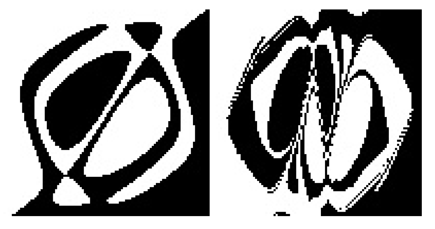
As
Table 6 shows, the only algorithm that coped with the TSP is HCAE(
Oper2) (example spirals generated by HCAE(
Oper2) networks are depicted in
Figure 4). In this case, ten runs ended with fully successful networks, and the average result amounts to 169. NEAT and CoSyNE, like AE and AEEO, appeared to be insufficiently effective to evolve even a single fully successful neural network. All NEAT and CoSyNE runs got stuck in more or less the same region of fitness function, that is, for NEAT, between 112 and 132 (example spirals generated by NEAT networks are depicted in
Figure 5), whereas for CoSyNE, between 96 and 106.
In IPP, HCAE(Oper2) again outperformed other methods. Generally, it had no problems with evolving fully successful networks that were able to balance the cart-and-pole-system for the maximal number of iterations in all four attempts. To evolve a fully successful network, it needed only 1386 network evaluations on average and 310 minimum.
Meanwhile, the rivals of HCAE, like in the previous case, could not successfully cope with the problem. The best result in both cases corresponds to the beginning of the second out of four simulations, that is, to the area of fitness function equal to 10,000. There were very few runs, in this case, that exceeded 11,000. As before, this result is very similar to those obtained by AE and AEEO.
Generally, two factors can be responsible for the difference in performance between HCAE and its rivals, i.e., the evolutionary algorithm and the encoding method. However, the most likely “suspect”, in this case, seems to be the evolutionary algorithm. As already mentioned, regardless of the testing problem, the results of NEAT and CoSyNE are very similar to those obtained by AE and AEEO. Meanwhile, the only thing that all the algorithms have in common is the traditional evolutionary model. This suggests that, like in the case of AE and AEEO, the decisive factor that prevented NEAT and CoSyNE from obtaining better results is the model of the evolution applied in both algorithms.
In turn, the influence of the encoding method is visible in the networks’ architecture: most networks evolved by NEAT and CoSyNE were densely connected with a maximum number of neurons. In the early stages of the evolution, NEAT produces “light” networks from “light” genetic representations. However, the representations and networks quickly become more and more complex and their effective processing more and more difficult. Exactly the same problem is observed in AE and AEEO, where the growth in genotypic complexity decreases the effectiveness of the evolution. In turn, CoSyNE, from the very beginning, evolves fully connected neurons of a fixed architecture and does not have any effective mechanism for producing sparse networks.
Meanwhile, the networks produced by HCAE(Oper2) often included fewer neurons than the assumed maximum size, and were very often sparse; NDMs of these networks contained many spacious holes filled with zeros.
4.7. Tests on Datasets from UCI Machine Repository
The most effective variant of HCAE was also compared with LFPSO, PSOLF, LPSONS, and BP on thirteen classification benchmarks from the UCI machine repository. To this end, HCAE was put to the test in the same conditions as those used in the experiments reported in [
27]. For each classification benchmark, the following setting was applied: 30 runs of the algorithm, neural networks with five hidden units, termination of the algorithm after 13,000 network evaluations, mean square error (MSE) as a minimized objective function, training set—80% and testing set—20% of data instances (in [
27]: 70%—testing set, 10% validation set, and 20% testing set).
Since the above conditions of the experiments assume a quick effect (only 13,000 network evaluations) with the use of small neural networks (only five hidden units), HCAE had to be adjusted to these conditions through appropriate parameter setting. First, the size of each NDM corresponded to networks with five hidden units. Second, it was assumed that, in order to evolve effective networks with a small number of neurons, the networks cannot be both small and sparse. In consequence, Oper2 was modified so as not to generate holes between consecutive values in NDMs. Third, in order to quickly evolve effective networks, the stagnation of the evolutionary process in CCEGA should be detected very quickly; the first symptoms of the stagnation should interrupt one evolutionary run and start a next run. To achieve such an effect, the interruption of each single CCEGA run took place after five iterations without progress.
Table 8 and
Table 9 show the comparison of all the five methods in terms of the training and testing accuracy that is defined in [
27] as a rate of correctly identified data instances to all instances derived either from the training or the testing set, respectively. In both tables, the best results for each benchmark are in bold.
The tables show that, in spite of unfavorable conditions for HCAE which is rather dedicated to problems which require greater networks and more effort to train them, it outperforms all rival methods in terms of both the training and testing accuracy. The number of wins (the best results in bold) for each algorithm and for each benchmark is as follows: training phase (BP = 0, PSOLF = 2, LFPSO = 3, LPSONS = 11, HCAE = 12), testing phase (BP = 6, PSOLF = 1, LFPSO = 2, LPSONS = 7, HCAE = 13), total (BP = 6, PSOLF = 3, LFPSO = 5, LPSONS = 18, HCAE = 25).
However, if the best accuracy is considered separately from the mean accuracy, the results are slightly different: training phase—best (BP = 0, PSOLF = 1, LFPSO = 2, LPSONS = 7, HCAE = 6), testing phase—best (BP = 4, PSOLF = 1, LFPSO = 2, LPSONS = 5, HCAE = 4), total—best (BP = 4, PSOLF = 2, LFPSO = 4, LPSONS = 12, HCAE = 10), training phase—mean (BP = 0, PSOLF = 0, LFPSO = 2, LPSONS = 4, HCAE = 6), testing phase—mean (BP = 2, PSOLF = 0, LFPSO = 0, LPSONS = 2, HCAE = 9), total—mean (BP = 2, PSOLF = 0, LFPSO = 2, LPSONS = 6, HCAE = 15). They show the high stability of HCAE which, regardless of the problem, the number of problem parameters, the number of data instances, and the starting point of the evolution, is able to quickly produce effective neural networks in almost every run. However, the above-mentioned result may also suggest some problems of HCAE with exploitation and finding globally optimal solutions. While the average effectiveness of HCAE is very high compared with other algorithms, its best networks were often inferior to the best networks of the rivals, especially to the networks of LPSONS.
4.8. Results of Experiments on the Trajectory-Following Problem
The aim of this phase of research was to verify the ability of HCAE to solve real problems requiring neural networks of small to medium size. Since one of the target applications of HCAE are control problems, it was decided that the real problem in this phase of the research would be to control a complex non-linear object, namely, an underwater vehicle. The rivals of the proposed algorithm in this case were DE and PSO, whose parameter setting is in
Appendix A, at the end of the paper. The task of each of the algorithms was the construction of the FFANN and RANN networks for the TFP problem described in
Section 4.3. Each of the algorithms was run 30 times and, during each run, it was possible to evaluate a maximum of 3,000,000 neural networks. The test results in the form of
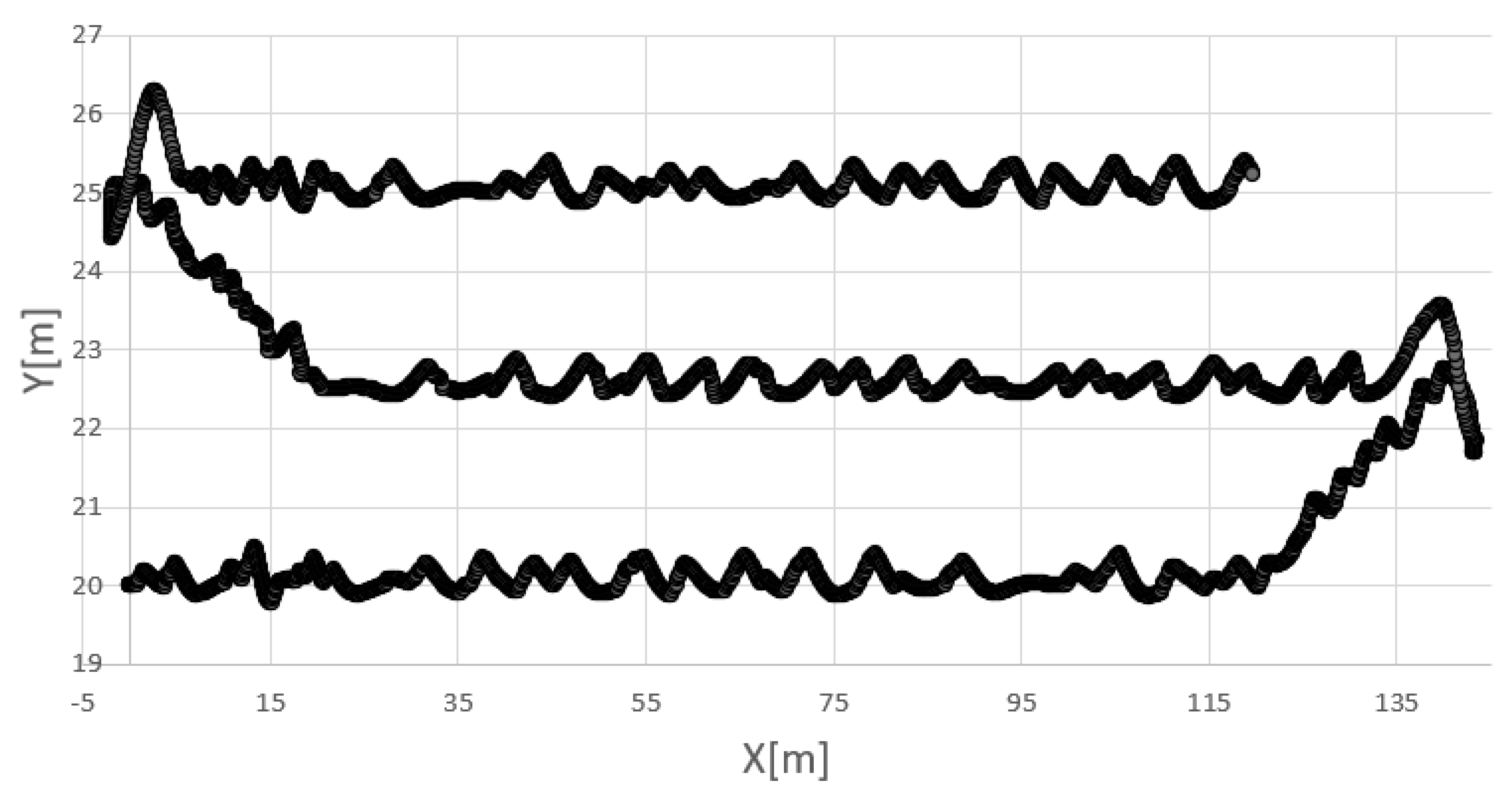
and
errors are presented in
Table 10, and an example of the AUV trajectory is shown in
Figure 6.
As can be seen, also in this case, the HCAE outperforms its rivals. The average and maximum errors and generated for all the 30 runs of the algorithm are definitely smaller than the errors obtained for the other algorithms, which proves that HCAE is able to very effectively solve not only artificial problems but also real ones. Moreover, the obtained result confirms the high efficiency of the new model of the evolution of neural networks proposed in the paper. The algorithms used in DE and PSO along with the direct network coding method used in them turned out to be less effective.
6. Conclusions
The paper presented a novel neuro-evolutionary algorithm called Hill Climb Assembler Encoding. The algorithm encodes a neural network in the form of a matrix which is filled with an evolutionary formed program called assembler encoding program. Like every assembler program, the AEP is composed of two parts, i.e., a part with implementation and a part with a data sequence. The implementation part includes operations whose code is fixed—it does not evolve. Each operation is supplied with a vector of parameters and a sequence of data. Both data and the parameters are shaped in the evolutionary way. Their evolution is conducted according to the CCEGA algorithm, one population includes data sequences, whereas vectors of parameters are processed in two other populations.
The HCAE has two variants which differ in applied operations. One variant uses so-called ANN operations, which are small neural networks whose task is to form the matrix representing a resultant neural network. The ANN operations are supplied with sequences of data. Another variant of HCAE does not use ANN operations; instead, it simply copies data directly to the matrix. Where data is copied and how much data is copied is determined by the operation.
HCAE was tested on fourteen classification problems, including the two-spiral problem, which is a well-known benchmark for binary classification and is regarded as extremely challenging, and on the inverted-pendulum problem which is a well-known control benchmark. In the tests, apart from HCAE, eight other algorithms were also used for comparison purposes, i.e., two predecessors of HCAE: essembler encoding, and assembler encoding with evolvable operations, and six other methods: Neuro-Evolution of Augmenting Topologies which is a well-known state-of-the-art NE method, Cooperative Synapse Neuro-Evolution, Levy Flight Particle Swarm Optimization (LFPSO), modified LFPSO, Mantegna Levy Flight, Particle Swarm Optimization, and Neighbourhood Search, and the classic Back-Propagation algorithm.
The experiments revealed that HCAE outperforms all rival methods. The main factor that decided the high effectiveness of HCAE compared with other algorithms is the gradual growth in the networks and neuro-evolution conducted in a reduced search space. HCAE constructs the networks incrementally, little by little, by gradually adding new neurons and connections to the best network found so far. Each increment is a product of other evolutionary runs, each of which processes very simple HCAE programs.
In contrast, in the remaining algorithms, we deal with a one-to-one relation between genotype and phenotype, resulting in each algorithm being responsible for finding a complete network in the genotype space. If the space is large and the problem is abundant with local minima, finding the optimum is not a trivial task. This applies particularly to direct methods such as NEAT or CoSyNE, which do not scale well with larger networks.
The HCAE variant, which constructs neural networks by locally expanding them with concentrations of neurons and connections, appeared to be the most effective. Another characteristic of this variant is extreme simplicity compared with other HCAE variants and other algorithms. To form a neural network, it simply copies data directly to the matrix representation of the network.
The global nature of ANN operations seems to be the main reason for the problems of the HCAE variant based on these type of operations with generating optimal networks. HCAE assumes a slow incremental growth in the networks in many successive evolutionary runs, whereas, ANN operations disprove this assumption with serious changes introduced to the networks, which can be very destructive for the connection schemes found earlier.


