1. Introduction
Autonomous mobile robots offer solutions to diverse fields, such as transportation, defense, industry, and education. Mobile robots can perform other tasks as well, including monitoring, material handling, rescue operations, and disaster relief. Autonomous robot navigation is also a key concept in industrial development for minimizing manual work. However, in most applications, the autonomous robot is required to work in an unknown environment, which may contain several obstacles in route to the desired distention.
Robot navigation involves the robot’s ability to determine its own location, direction, and path to the destination. For most of the navigation tasks, mobile robots are required to read the environment based on sensor readings and prior knowledge. The formulation of this representation and the creation of a map, called Simultaneous Localization and Mapping (SLAM), was first addressed in [
1,
2].
In general, robots are expected to operate in autonomously in dynamic and complex environments. Understanding the environment’s characteristics is a significant task to allow the robot to move autonomously and make suitable decisions accordingly. Recently, the mobile robotics field has started to incorporate semantic information into navigation tasks, leading to a new concept called semantic navigation [
3]. This kind of navigation brings robots closer to the human way of modeling and understanding the navigation environment, representing the navigation environment in a human-friendly way.
Semantic knowledge has created new paths in robot navigation, allowing a higher level of abstraction in the representation of navigation information. In robot navigation, semantic maps offer a representation of the environment considering elements with high levels of abstraction. Most of the recently developed semantic approaches divide the indoor environments into three categories [
4]: rooms, corridors, and doorways, as these are the three most representative semantic labels on the 2D map. According to [
5], semantic navigation offers significant benefits to the area of mobile robot navigations, as follows:
Human-friendly models: The mobile robot models the environment in a way that humans understand.
Autonomy: The mobile robot can decide, on its own, how to travel to the designated location.
Efficiency: Calculating the route to the destination does not require the robot to explore the entire environment. Instead, it focuses on specific areas for partial exploration.
Robustness: The mobile robot can recover missing information.
Understanding the environment is an essential task to perform high-level navigation; therefore, this paper focuses on the semantic information for mobile robot navigation. We developed a semantic classification system that can distinguish between four different environments (rooms, doors, halls, and corridors) based on LiDAR data frames, and it can be employed in indoor navigation approaches. The developed semantic classification system consists of two main phases: offline and online. In the former phase, the dataset is collected from four different environments, labeled, processed, and trained using Machine Learning (ML) models, whereas in the later phase, the testing process is taken place to assess the efficiency of the developed classification system. Thus, the main contributions of this paper are as follows:
Research on recently developed semantic-based navigation systems for indoor environments.
Building a semantic dataset that consists of indoor LiDAR frames collected from a low-cost RPLiDAR A1 sensor.
Adopting a preprocessing method to maintain the collected LiDAR data frames.
Investigating the accuracy of semantic classification using several ML models.
The rest of this paper is organized as follows:
Section 2 discusses the recent developed semantic navigation systems employed in mobile robotics, whereas
Section 3 presents the developed semantic classification model.
Section 4 discusses the experiment testbed including the robot system and the environment structures. In
Section 5, we discuss the obtained results of the proposed system, and finally,
Section 6 concludes the work presented in this paper and suggests future work.
2. Related Works
In general, the robot navigation systems can be categorized into three categories: geometric-based navigation, semantic-based navigation, and hybrid (geometric and semantic). Geometric-based navigation uses geometric features or grids to describe the geometric layout of the environment, whereas the semantic-based navigation involves abstraction and includes vertices which correspond to places and edges in the environment. The hybrid category employs geometric information along with semantic knowledge to represent the environment by, for instance, employing range-finder sensors for metric representation while also using a digital camera to obtain semantic information about the environment.
Although the LiDAR frames are simple and easy to obtain, they can be employed to perform semantic classification for several environments; LiDAR sensors have been deployed in various classification projects. For instance, the authors of [
6] proposed a new approach for road obstacle classification using two different LiDAR sensors. Moreover, the works presented in [
7,
8] developed classification systems for forest environment characteristics, whereas in [
9], the authors used a single LiDAR sensor to maintain the continuous identification of a person in a complex environment. The author of [
10] developed a classification system using a LiDAR sensor, which was able to classify three different types of buildings: single-family houses, multiple-family houses, and non-residential buildings. The obtained classification accuracy was >70%.
The work presented in [
11] developed a method for pointwise semantic classification for the 3D LiDAR data into three categories: non-movable, movable, and dynamic objects. In [
12], the authors proposed a 3D point cloud semantic classification approach based on spherical neighborhoods and proportional subsampling. The authors showed that the performance of their proposed algorithm was consistent on three different datasets acquired using different technologies in various environments. The work presented in [
13] utilized a large-scale dataset named SemanticKITTI, which showed unprecedented scale in the pointwise annotation of point cloud frames.
Recently, the rapid development of deep learning in image classification has led to significant improvements in the accuracy for classifying objects in indoor environments. Several powerful deep network architectures have been proposed recently, including GoogleNet [
14,
15], VGGNet [
16], MobileNet [
17], and ResNet-18 [
18] to solve the problem of image classification. For instance, the authors of [
19] proposed an object semantic grid mapping system using 2D LiDAR and an RGB-D camera. The LiDAR sensor is used to generate a grip map and obtain the robot’s trajectory, whereas the RGB-D camera is employed to obtain the semantics of color images and employ joint interpolation to refine camera poses. The authors employed the Robot@Home dataset to assess the system’s efficiency and used the R-CNN model to detect static objects such as beds, sinks, microwaves, sinks, toilets, and ovens.
In [
20], the authors proposed a framework to build an enhanced metric representation of indoor environments. A deep neural network model was employed for object detection and semantic classification in a visual-based perception pattern. The output of the developed system was a 2D map of the environment extended with semantic object classes and their locations. This system collected the required data from several sensors including LiDAR, an RGB-D camera, and odometers. In addition, the authors employed CNN-based object detection and a 3D model-based segmentation technique to localize and identify different classes of objects in the scene.
The work presented in [
21] included the development of an intelligent mobile robot system which was able to understand the semantics of human environments and the relationships with and between humans in the area of interest. The obtained map offered a semi-structured human environment that provided a valuable representation for robot navigation tasks. Moreover, the obtained map consisted of high-level features, such as planar surfaces and door signs that involve text and objects.
The authors of [
22] proposed a self-supervised learning approach for the semantic segmentation of LiDAR frames. Through this study, the authors revealed that it was possible to learn semantic classes without human annotation and then employ them to enhance the navigation process. The work presented in [
23] developed a CNN model for classifying objects and indoor environments including rooms, corridors, kitchens, and offices using visual semantic representations of the data received from the vision sensor.
In [
24], the authors proposed a probabilistic approach integrating heterogenous, uncertain information such as the size, shape, and color of objects through combining the data from multi-modal sensors. This system employed vision and LiDAR sensors and combined the received data to build a map. The work presented in [
25] used a semantic relational model that involved both the conceptual and physical representation of places and objects in indoor environments. The system was developed using a Turtle robot with onboard vision and LiDAR sensors.
In [
26], the authors employed image sensors for path planning based on the movable area extraction from input images using semantic segmentation. The experimental results proved that the ICNet could extract the moveable area with an accuracy of 90%.
The authors of [
27] proposed a low-cost, vision-based perception system to classify objects in the indoor environment, converting the problem of robot navigation into scene understanding. The authors designed a shallow convolutional neural network with efficient scene classification accuracy to process and analyze images captured by a monocular camera.
The work presented in [
28] analyzed the relationship between the performance of image prediction and the robot’s behavior, which was controlled by an image-based navigation system. In addition, the authors discussed the effectiveness of directing the camera into the ceiling to adapt to dynamic changes in the environment.
As stated above, most of the recently developed systems are based on the integration of visual and LiDAR representations of the environment.
Table 1 presents a comparison between the research works discussed in this section according to the type of employed sensors, the number of classification environments and objects, and the obtained accuracy.
3. Semantic Classification System
In this work, we developed a semantic classification model for robot navigation that can recognize the navigation area using a low-cost, LiDAR-based classification system. The developed system can differentiate between four different environments: rooms, corridors, doorways, and halls.
The developed semantic classification system consists of two main phases: offline and online. In the offline phase, the LiDAR data frames are collected, processed, stored in a database file, and used as a training dataset for ML models, whereas in the online phase, the robot collects the LiDAR data, processes it, and then classifies the environment type (room, doorway, corridor, or hall) according to the pretrained model in the offline phase.
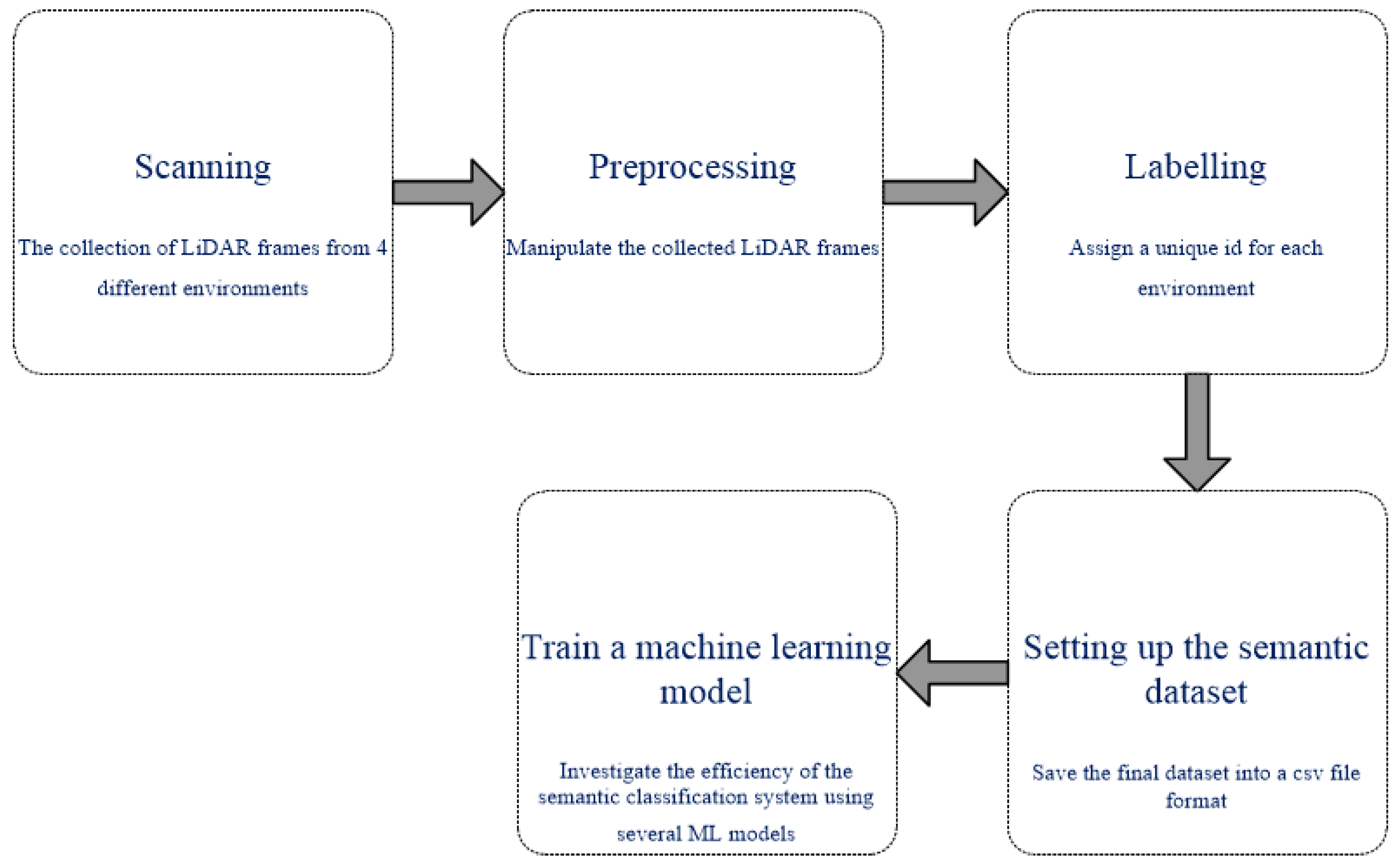
Figure 1 shows the concept of the proposed semantic classification model (offline phase), which consists of five main stages, as follows:
The collection of LiDAR frames: The mobile robot scans the environment using RPLiDAR A1 and collects 360 different samples for each environment. However, in most of the cases, the scanned LiDAR data consist of missing and infinity values, which can be obtained from either very far or very close walls/objects, and this may reduce the accuracy of the classification model.
Process the collected data: Since the scanned LiDAR data consist of missing and infinity values, it is important to recover the missing values and process the infinity values to guarantee high classification accuracy. Algorithm 1 presents the recovery function that has been employed to process the missing data, which runs on a Raspberry Pi computer. The missing data are processed according to the LiDAR data frames that exist before and after the missing data frame(s), where in certain cases, the missing data frames are either averaged or replicated according to the position and the quantity of the missing data frames.
Label the processed data: The developed semantic classification system will be able to classify between four different environments: doorways, rooms, corridors, and halls. Therefore, each environment has been assigned a unique identification number (label) as presented later (for instance, room: 0, corridor: 1, doorway: 2, and hall: 3).
Store the labeled data: The processed LiDAR frames are stored in a csv file to make it available for the training phase.
Figure 2 presents the structure of the processed LiDAR frames received from the LiDAR sensor after the processing stage.
Train the model: This phase involves employing several ML models to train and test the efficiency of the developed semantic classification system using various metrics.
| Algorithm 1: Preprocessing phase of the sensed LiDAR data |
| Input: Array of LiDAR frames with the size of 360 values |
| Output: Processed LiDAR frames with the size of 360 values |
| 1: let frames[] is a 1D array of the LiDAR frames |
| 2: let cols is the total number of received frames |
| 3: let count = 0 is a loop counter |
| 4: let max is the maximum number in a set of LiDAR values |
| 5: let loc is the initial index for the first ‘inf’ value |
| 6: while (frames[count] < cols) |
| 7: if(frames[count] == ‘inf’) |
| 8: loc = count |
| 9: if(count == 0) |
| 10: max = 0 |
| 11: else: max = frames[count-1] |
| 12: while(frames[count] == ‘inf’) |
| 13: count++ |
| 14: if(max < frames[count]) |
| 15: max = frames[count] |
| 16: while(count ≥ loc) |
| 17: frames[count] = max |
| 18: count-- |
| 19: count += loc |
| 20: end |
The online phase involves collecting LiDAR frames from the LiDAR sensor, processing the collected data, and then classifying the environment type (where the robot is located) according to the pretrained model in the offline phase. This proceeds as follows:
Scan the area of interest: The LiDAR frames from the area where the mobile robot is placed are scanned.
Process the collected data: The collected data contain missing and infinity values; therefore, Algorithm 1 is employed to recover these values.
Classify the environment type: The processed LiDAR frames are passed to the pretrained model to classify the environment type.
4. Experimental Testbed
This section discusses the experiment testbed including the mobile robot system, the labeling phase, and the collection procedure of the LiDAR frames from four different types of environments.
4.1. Mobile Robot System
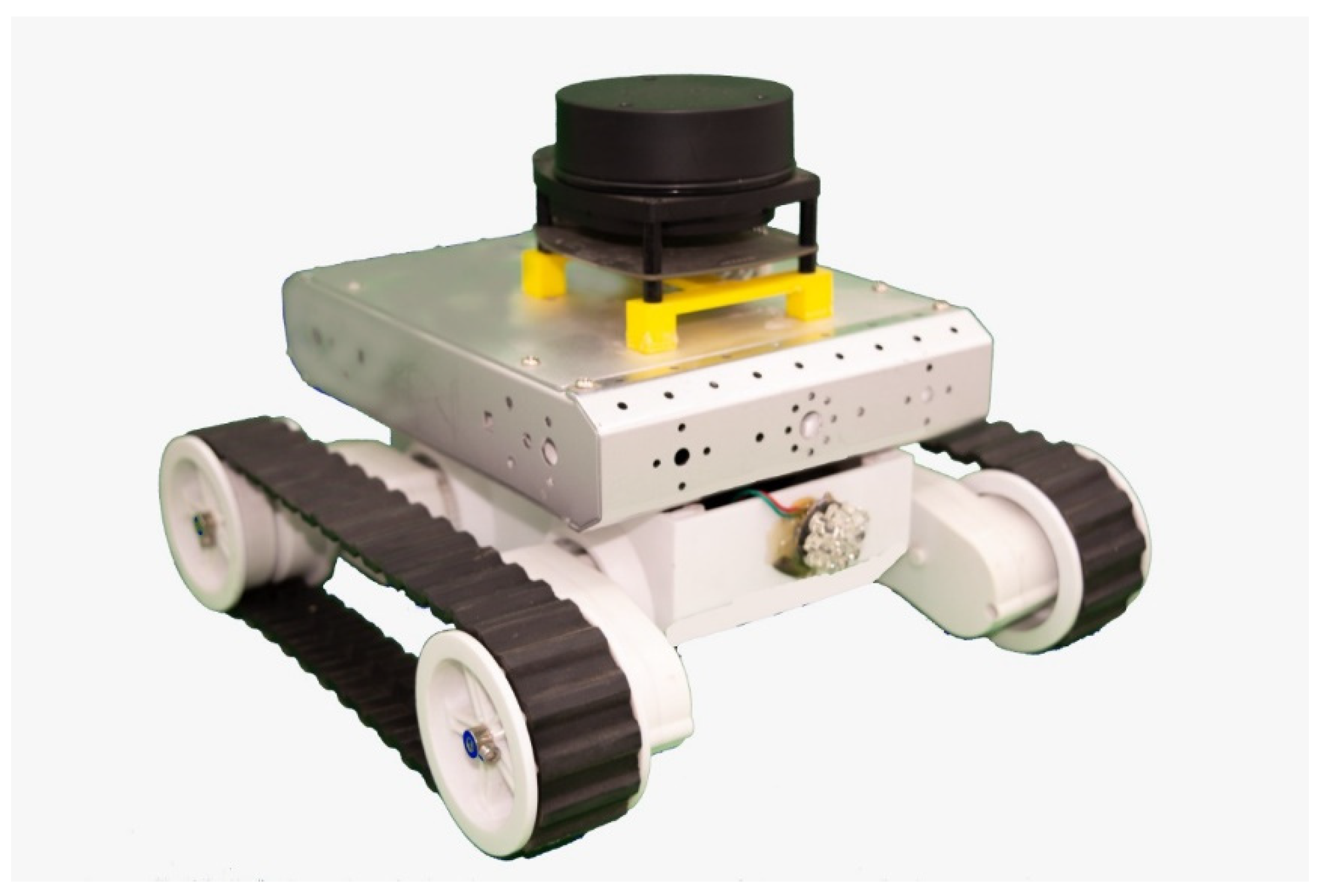
This section presents the mobile robot system employed in our experiments. The employed mobile robot is a four-wheel drive robot equipped with a 2D laser (RPLiDAR A1), which is high-speed vision acquisition and processing hardware developed by SLAMTEC. It can achieve 360° scans within a 12 m range and generate 8000 pulses per second.
Figure 3 depicts the developed mobile robot system employed in our experiments. The mobile robot was able to freely move in the area of interest based on range finder sensors.
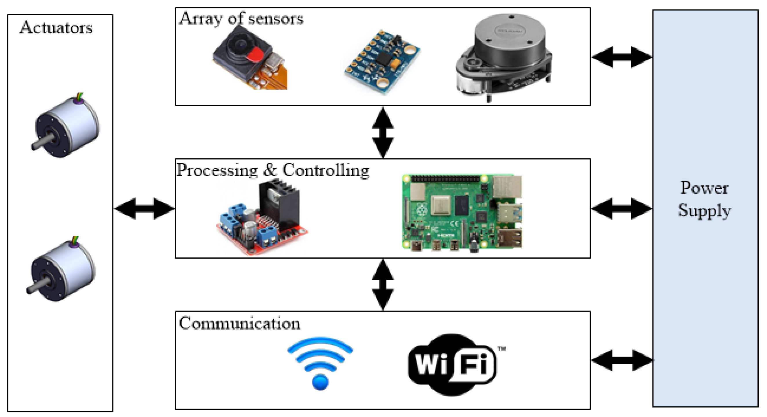
The mobile robot system consists of a Raspberry Pi 4 4-GB RAM computer, an array of sensors (gyro, motor-encoder, and RPLiDAR), a motor driver, and four-wheel drive motors. The mobile robot architecture is presented in
Figure 4.
Table 2 shows the full specifications of the employed RPLiDAR A1, whereas
Table 3 presents the full specifications for the employed Raspberry Pi 4 computer system. The onboard Raspberry Pi 4 computer collects the LiDAR frames from the RPLiDAR sensor, preprocesses the received frames, and then employs an ML model to identify the environment class.
With regard to software requirements, the developed semantic classification system integrates several software development kits including Python 3.7.13 as a development environment, Pandas 1.3.5 for processing the LiDAR frames, and a Numpy 1.21.6 library for working with arrays.
4.2. Setting up the Semantic Information Dataset
Recognizing places and objects is a complicated task for robots. Therefore, there are several methods to complete object identification tasks. As mentioned earlier, the proposed semantic classification system can distinguish between four different environments (rooms, doorways, corridors, and halls). First, the room dataset was collected from 43 different rooms, where most of the rooms were furnished and included cabinets, beds, chairs, and desks. The rooms’ size was in the range of 3.5 × 3.5 m.
Second, the corridor dataset was collected from 51 different corridors located in different places (Faculty of Computers & Information Technology building, Industrial Innovation & Robotics Center, and other corridors located in the University of Tabuk). In the corridor dataset, the ratio of infinity values was around 5.89%, and this is because one, one or two sides of the corridors may be out of range, and two, the RPLiDAR A1 may offer inaccurate readings in some situations.
Third is the doorway dataset. This involves collecting the LiDAR frames from almost 63 different doors (opened status). In most cases, the door dataset was collected from rooms, corridors, and halls with opened doors. The infinity ratio in the doorway dataset was around 2.76%; as with the room dataset, most of the LiDAR frames are in the range of the RPLiDAR A1 sensor.
Fourth, the hall dataset was collected from different halls located in the University of Tabuk, including: lecture halls, open space halls, and large labs, with a total number of 49 different halls. In the hall dataset, the ratio of infinity values is around 20.32%, since in some cases, the LiDAR frames were out of range.
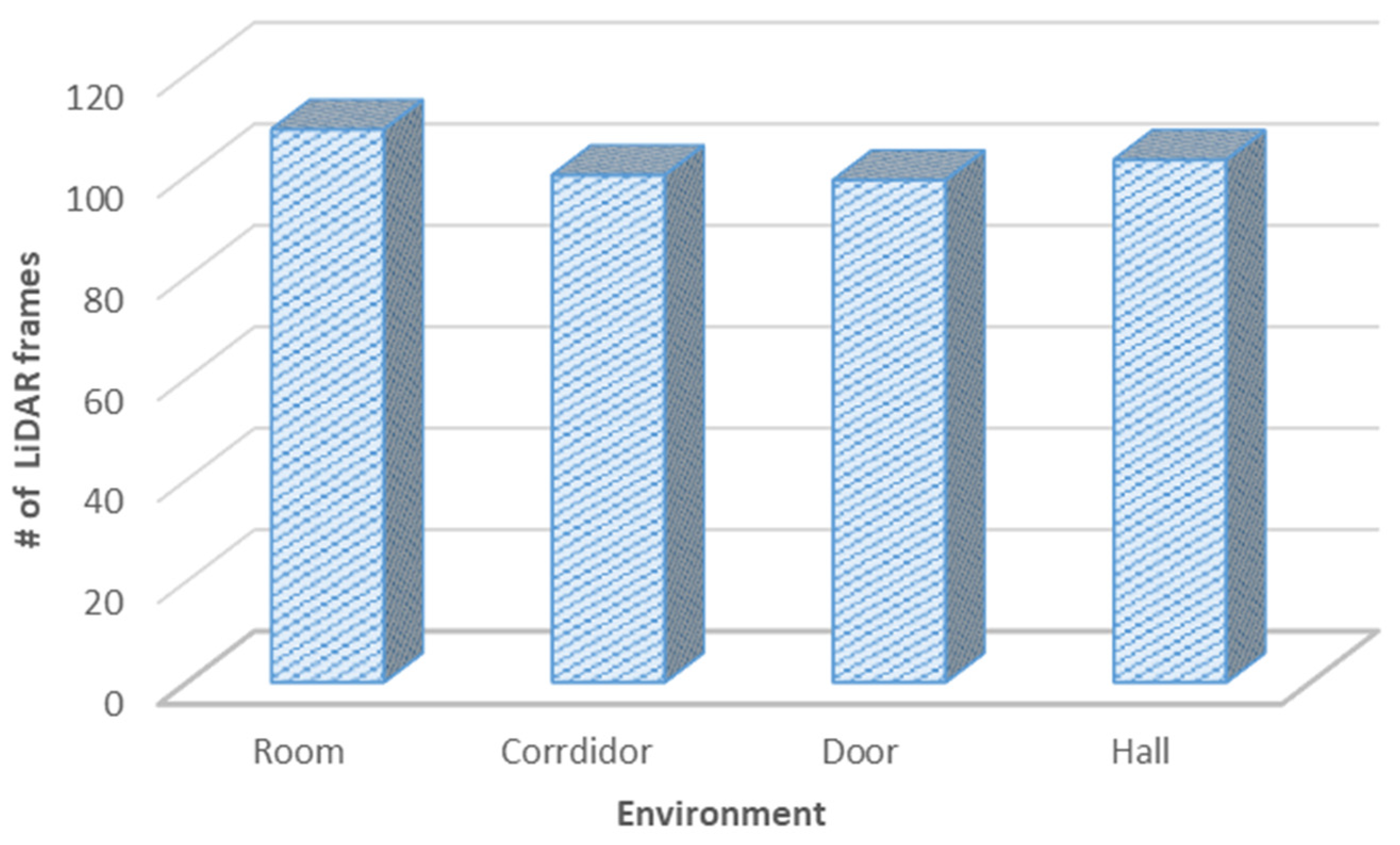
Figure 5 shows the total number of records for each class (environment), where the total amount of collected data from each environment is almost equal to the other classes. As shown below, the established dataset with four classes is almost balanced, with the following records: 109, 100, 99, and 103 for rooms, corridors, doorways, and halls, respectively.
Table 4 presents general statistics about the number of collected readings from different environments.
Figure 6 shows an example of the hall, room, corridor, and door environments.
The labeling process has been completed manually by labeling each environment separately with a unique identifier (0: room, 1: corridor, 2: doorway, and 3: hall). The results were then saved in a database file.
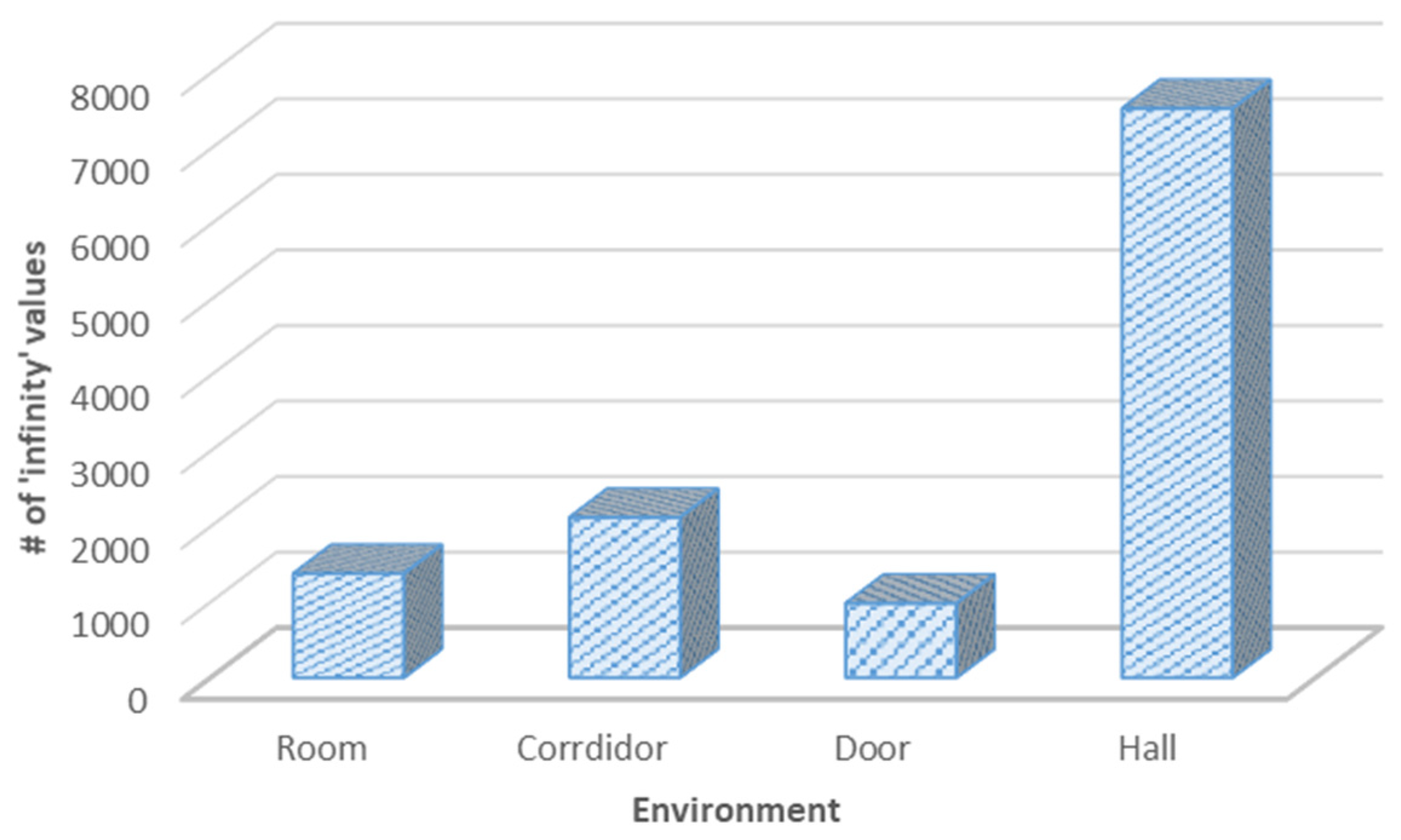
One of the main limitations of the RPLiDAR A1 ranging sensor is that this type of sensor may provide infinity and missing values when scanning, which leads to inaccurate semantic information and thus an inefficient robot navigation system. Therefore, in this section, we presented measurements for the “infinity” values received by each class.
Figure 7 shows the total number of “infinity” values for each environment class, where the ratio of infinity values differs from one environment to another; however, there is no noticeable variation between the corridor, doorway, and room classes, whereas a large difference is shown between the first three classes (room, corridor, and doorway) and the fourth class (hall), because the hall areas were, in general, larger than the range of the RPLiDAR A1.
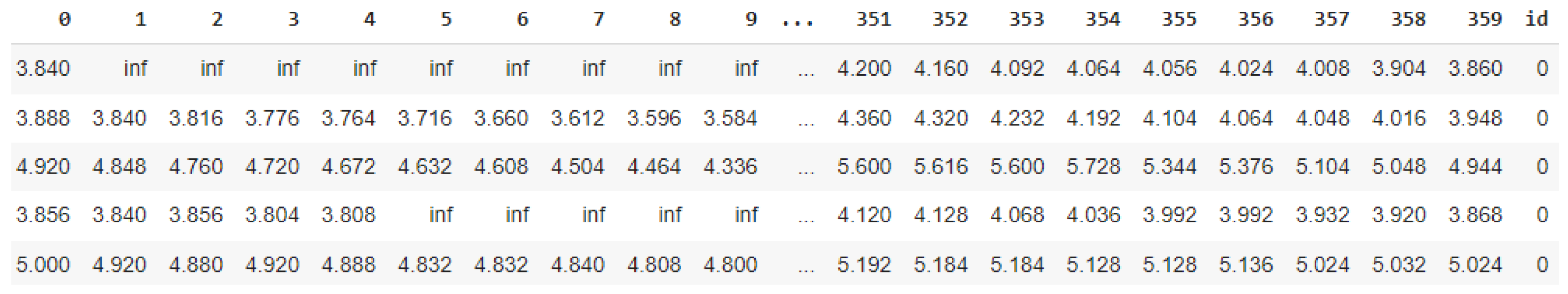
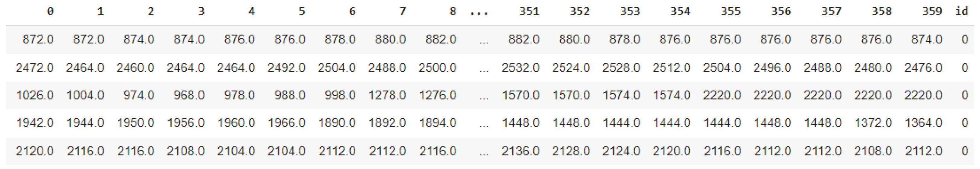
Figure 8 depicts the collected LiDAR data frames from the RPLiDAR A1 for the room environment, which consists of several ‘infinity’ values obtained from close or out of range objects. The processed LiDAR frames are presented in
Figure 9, where the ‘inf’ values were processed with numerical values according to the preprocessing function presented in Algorithm 1.
4.3. Machine Learning Algorithms
This section discusses the employed ML models, including decision tree, CatBoost, random forest (RF), Light Gradient Boosting (LGB), Naïve Bayes (NB), and Support Vector Machine (SVM).
Recently, ML methods have played a significant role in the field of autonomous navigation, where ML techniques have provided a robust and adaptive navigation performance while minimizing development and deployment time. In this work, we tried several ML models to train, test, and classify the environment type using the developed semantic classification approach in order to find the best performance among them. The following ML models have been employed:
Decision Tree: The decision tree model is a tree-like structure that allows you to make a decision on a given process. The flowchart starts with a main idea and then branches out based on the consequences of the final decision. We employed decision tree because it is a powerful method for classification and prediction, and it can handle non-linear datasets in an effective way. In our experiments, the training parameter for the decision tree is the max depth (max_depth = 16).
CatBoost: The CatBoost classifier is based on gradient boosted decision trees. In the training phase, a set of decision trees is built consecutively. Each successive tree is built with reduced loss compared to the previous trees. Usually, CatBoost offers state-of-the-art results compared to existing ML models, and it can handle categorical features in an autonomous way. For the implemented CatBoost classifier, the training parameters are presented in
Table 5.
Random Forest (RF): The random forest is a classification algorithm made up of several decision trees. Each individual tree is built in a random way to promote uncorrelated forests, which then employ the forest’s predictive power to offer an efficient decision. The random forest has been employed in our system, since it is useful when dealing with large datasets, and interpretability is not a major concern. The training parameters for the implemented RF classifier are presented in
Table 6.
Light Gradient Boosting (LGB): This is a decision tree-based method. It is a fast, distributed, high-performance gradient boosting framework. In this work, we employed Light Gradient Boosting because it achieves high accuracy when the classifier is unstable and has a high variance. The training parameters for the implemented LGB classifier are presented in
Table 7.
Naïve Bayes (NB): This is based on the Bayes theorem to classify the objects in the dataset. The Naïve Bayes classifier assumes powerful, or naïve, independence between attributes of data points. We have employed Naïve Bayes because it employs similar methods to predict the probability of different classes based on various attributes.
Support Vector Machine (SVM): The SVM maps data to a high-dimensional feature space, so the data points can be categorized, even if the data are not linearly separable. SVM is effective in high-dimensional spaces, and it uses a subset of training points in the decision function. In addition, SVM is an efficient model in terms of memory requirements. The training parameters for the implemented Support Vector Machine classifier are presented in
Table 8.
5. System Evaluation
This section details the training and testing phases of the classification process. The collected dataset has been divided into two subsets: training and testing, with 70% for training and 30% for testing (287 and 124 records for training and testing, respectively).
The proposed algorithms’ performance is tested and evaluated using the collected LiDAR frames dataset, which consists of 411 data frames distributed among four different class environments. For evaluation purposes, we assessed the performance of the ML model through different metrics, including:
Confusion matrix: This describes the complete performance of the environment classification model.
Accuracy: This refers to the percentage of the total number of environment classes that were correctly predicted. Accuracy defines how accurate the environment classification system is. The accuracy formula is presented below:
where
cp and
t refer to the correct predictions and the total number of samples, respectively.
Precision: This refers to the ratio of correctly predicted positive observations over the total predicted positive observations. For multi-class classification, there are two different approaches to compute the precision:
Recall: This refers to the ratio of correctly predicted positive observations to all the observations in the actual class. In multi-class classification, the recall is estimated in two different ways, as follows:
F1-score: This refers to the weighted average of precision and recall. An F1-score is more useful than accuracy if the dataset is unbalanced. However, in our case, the environment classes are almost balanced. The F1-score can be calculated in two different ways:
Receive Operating Characteristic (ROC): This refers to the performance measurement for classification problems at different threshold settings.
5.1. Confusion Matrix
The confusion matrix for each ML model has been obtained to assess efficiency in the testing phase. For instance,
Table 9 shows the confusion matrix for the NB classifier, where the classifier could classify the rooms, corridors, and halls with high classification accuracy; however, the classification accuracy for the doorway class was only reasonable.
On the other hand,
Table 10 presents the confusion matrix for the RF classifier, with better classification accuracy than the NB classifier for both the corridor and doorway classes. In
Table 11, the confusion matrix for the CatBoost classifier is presented, where an efficient classification accuracy was obtained for identifying the room, corridor, and hall classes, whereas the door class received a low classification accuracy.
Table 12 shows the confusion matrix for the decision tree classifier, where the classifier offers reasonable classification accuracy for the room, corridor, and hall classes, whereas the doorway offered the minimum classification accuracy. The confusion matrix for the LGB classifier is presented in
Table 13, where the obtained classification accuracy was reasonable for all classes except the doorway calls. Finally,
Table 14 presents the confusion matrix for the SVM classifier. As noted, the SVM offers the best classification accuracy for almost classes.
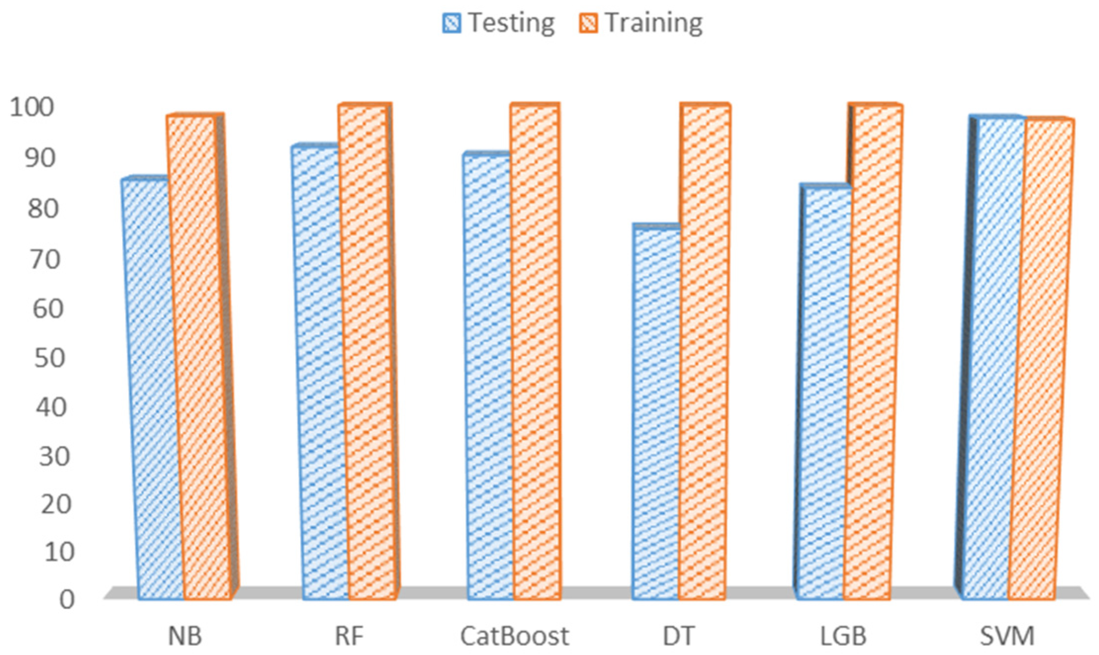
5.2. Classification Accuracy
The classification accuracy is a significant metric in this project, as the collected LiDAR dataset contains an almost equal number of samples for each environment (class). Therefore, the classification accuracy has been assessed for both the training and testing phases, as shown in
Figure 10.
The training accuracy, along with several performance metrics for the employed ML models, is presented in
Table 15. As noted, RF, CatBoost, decision tree, and LGB offer 100% training accuracy, whereas NB offers the minimum training accuracy with 90.97%, and SVM achieves 96.86% training accuracy.
We also evaluated the testing accuracy for all ML models.
Table 16 presents several evaluation metrics for each ML model. In terms of accuracy, SVM achieves the best classification accuracy of 97.21% using the testing subset, whereas decision tree offers the minimum accuracy 75.80%. In general, SVM offers high classification accuracy when there is a clear margin of separation between classes.
5.3. Precision, Recall, and F1-Score
In addition to the classification accuracy, the precision, recall, and
F1-scores all have been assessed for each ML model in the training phase. As noticed in
Table 15, the RF, CatBoost, decision tree, and LGB offer the best precision, recall, and
F1-score results with a score of almost 99.99%, whereas the NB classifier achieves the worst results with an average score (precision, recall, and
F1-score) of 93.29%. The SVM classifier offers efficient scores (precision, recall, and
F1-score), with an average score of 98.89%.
The precision, recall, and F1-score indicators are also computed for the testing phase. In this case, precision represents the quality of the positive predictions made by the ML model. The SVM classifier offers the best precision among all the ML models, with an average precision of 97.24%, whereas the RF classifier comes in second with an average precision of 92.17%. Decision tree achieves the worst precision score among all the ML models, at 75.55%.
Unlike prevision scores, recall provides a measure of how accurately the ML model was able to identify the relevant data. The SVM classifier offers the best recall score among the six ML models, at 97.48%. However, recall scores are not as significant as accuracy, since the established dataset is balanced. The
F1-score was also computed; it sums up the predictive performance of an ML model by combining the recall and precision scores. According to the presented results in
Table 16, the SVM model achieves the best
F1-score results, at 97.34%.
5.4. Receiver Operating Characteristic (ROC)
This section discusses the ROC by analyzing the performance of six classification models at different classification thresholds, as presented in
Figure 11. As discussed earlier, SVM offers the best accuracy, precision, recall, and
F1-scores. However, the ROC is a significant metric to assess the performance of predicting each class separately.
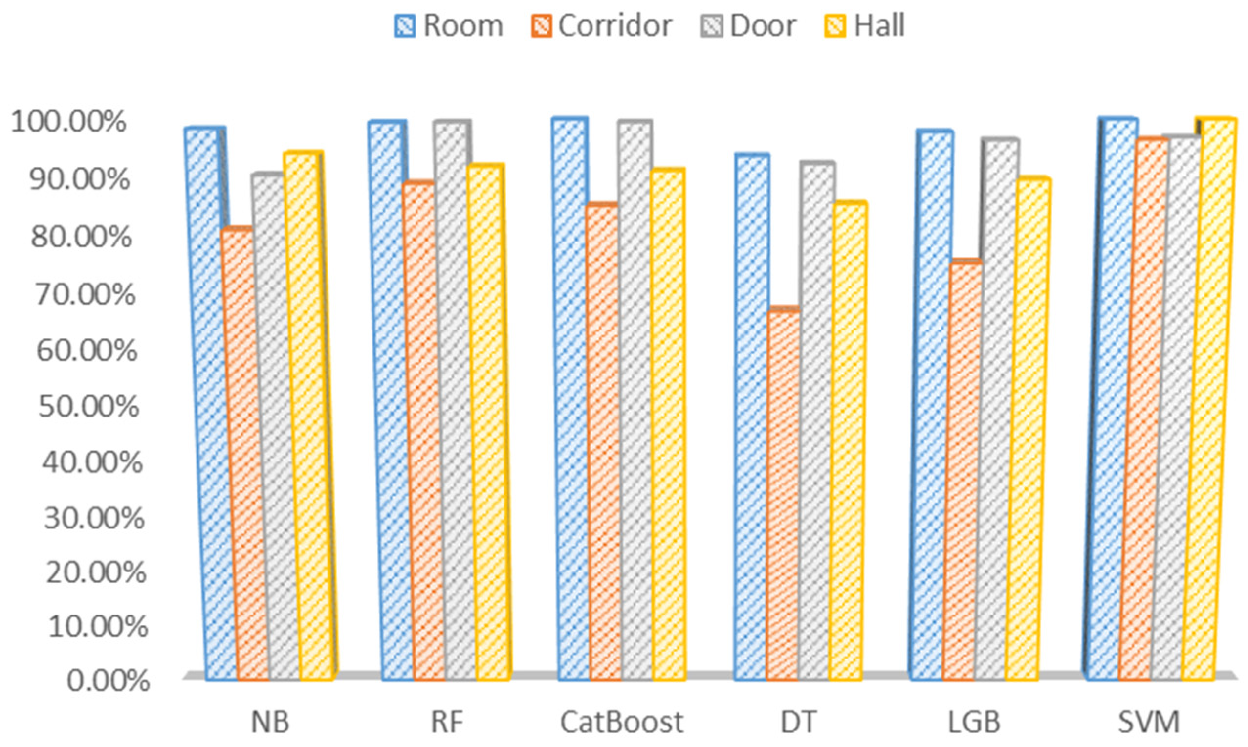
Table 17 presents the evaluation of ROC for all ML models, where the SVM classifier offers the best classification accuracy for the room, doorway, and hall environments, at 100.0%, 96.50%, and 100.0%, respectively. SVM, on the other hand, offers a reasonable identification accuracy for classifying the door class with an accuracy of 96.91%. The RF and CatBoost classifiers offer the best classification accuracy for the corridor class with an accuracy of 99.50% for both models. Moreover, CatBoost achieves similar classification accuracy on the hall class. Therefore, CatBoost comes in second place after SVM.
6. Discussion
The importance of this research is to study the benefits of the information collected using our RPLiDAR A1 sensor to better grasp the semantic information for a navigation robot’s traversed environment.
In this research, we were able to develop a system based on ML algorithms, through which we can distinguish the environment surrounding the robot including four different areas: rooms, corridors, doorways, and halls using a range-finder sensor. We were able to achieve a high accuracy rate of 97.21% utilizing the SVM model after testing with a variety of machine-learning techniques. Our goal, as stated in the introduction, is to provide a low-power, high-performance navigation system that can run on a Raspberry Pi 4 computer, and this is what we achieved.
In comparison with the developed semantic-based vision systems [
19,
20,
21,
22,
23,
24,
25,
26], the authors employed deep learning using vision camera sensors to build a semantic navigation map for robot systems, with a reasonable classification accuracy, where the average classification environments/objects were equal to (4–8) classes, with a reasonable classification accuracy (average classification accuracy of 83%). However, these architectures require powerful GPUs, large memories, and huge datasets, which make these solutions difficult to deploy on low-power devices.
In fact, we were unable to compare the results we obtained in this study with the results of other researchers’ work in this field due to a number of factors, the most important of which is the lack of a general dataset with which we can compare the results, as well as a different research structure. This research tried to rely on low-power, high-performance navigation systems, which do not currently exist in the field.
Furthermore, the results obtained in this paper, which showed that the SVM algorithm is superior to the other employed algorithms, are due to several factors, the most important of which is the nature of the data used, which is somewhat separated from each other, making it easier for the algorithm to classify with high accuracy.
7. Conclusions
In this research, we effectively improved the ability of a robot to achieve a broader understanding of the environment surrounding it by distinguishing four areas in which the robot may be located, which are rooms, corridors, doorways, and halls. The developed system was built on a low-power and high-performance navigation approach to label the 2D LiDAR room maps for better and more effective semantic robot navigation. Although many ML algorithms were used in distinguishing the collected data from the RPLiDAR A1 sensor, we found that the support vector machine algorithm achieved the highest accuracy in both the training and testing phases.
Further semantic information—through adopting additional range-finder sensors, building a large enough indoor dataset with more environment classes, and investigating more ML algorithms—will be important directions in future work.


 and
and 


