
Active Mask-Box Scoring R-CNN for Sonar Image Instance Segmentation


Abstract
:1. Introduction
2. Related Work
2.1. Mask Scoring R-CNN
2.2. Active Learning
3. Materials and Methods
3.1. M-B Scoring R-CNN
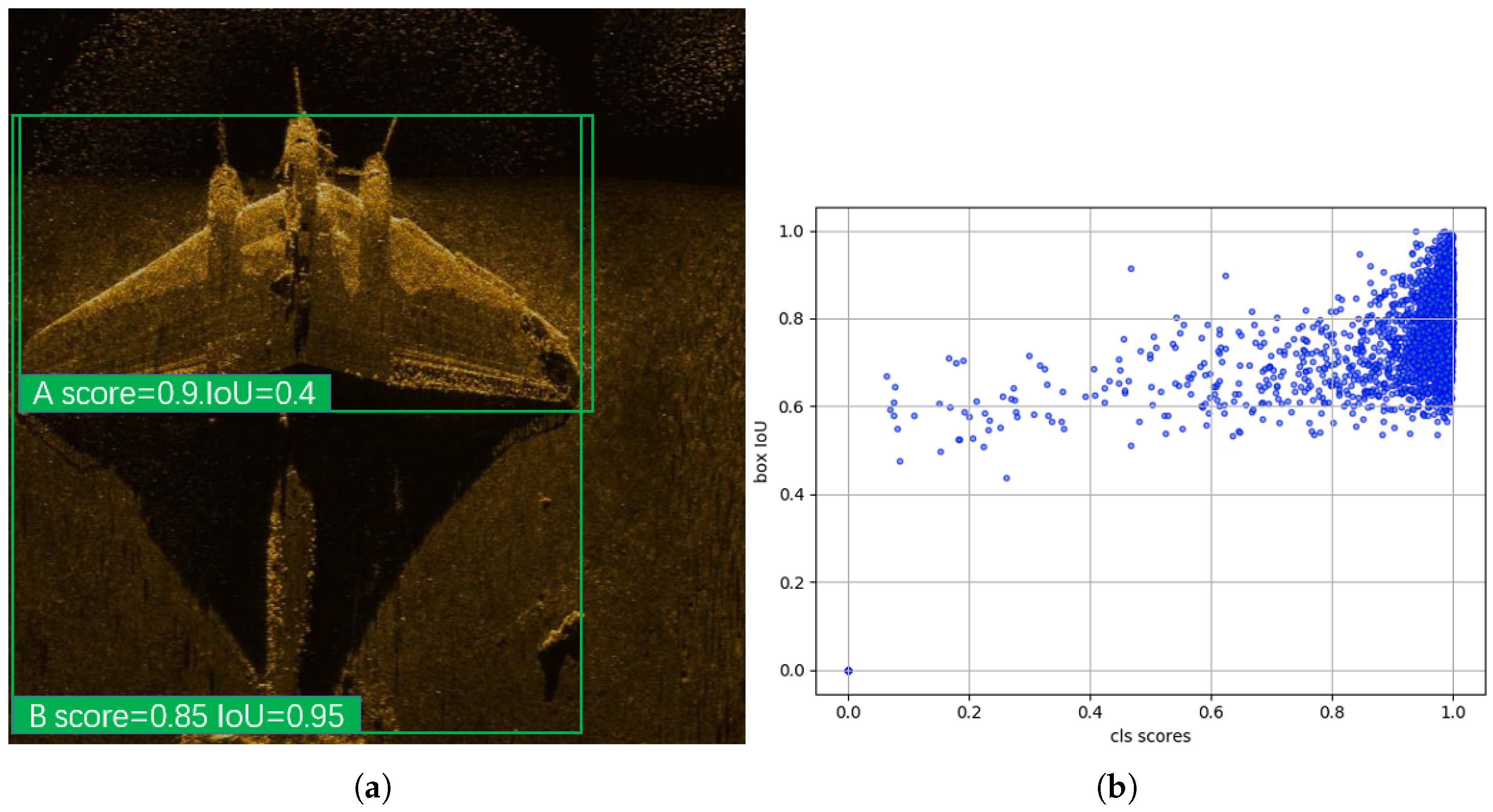
3.1.1. Motivation
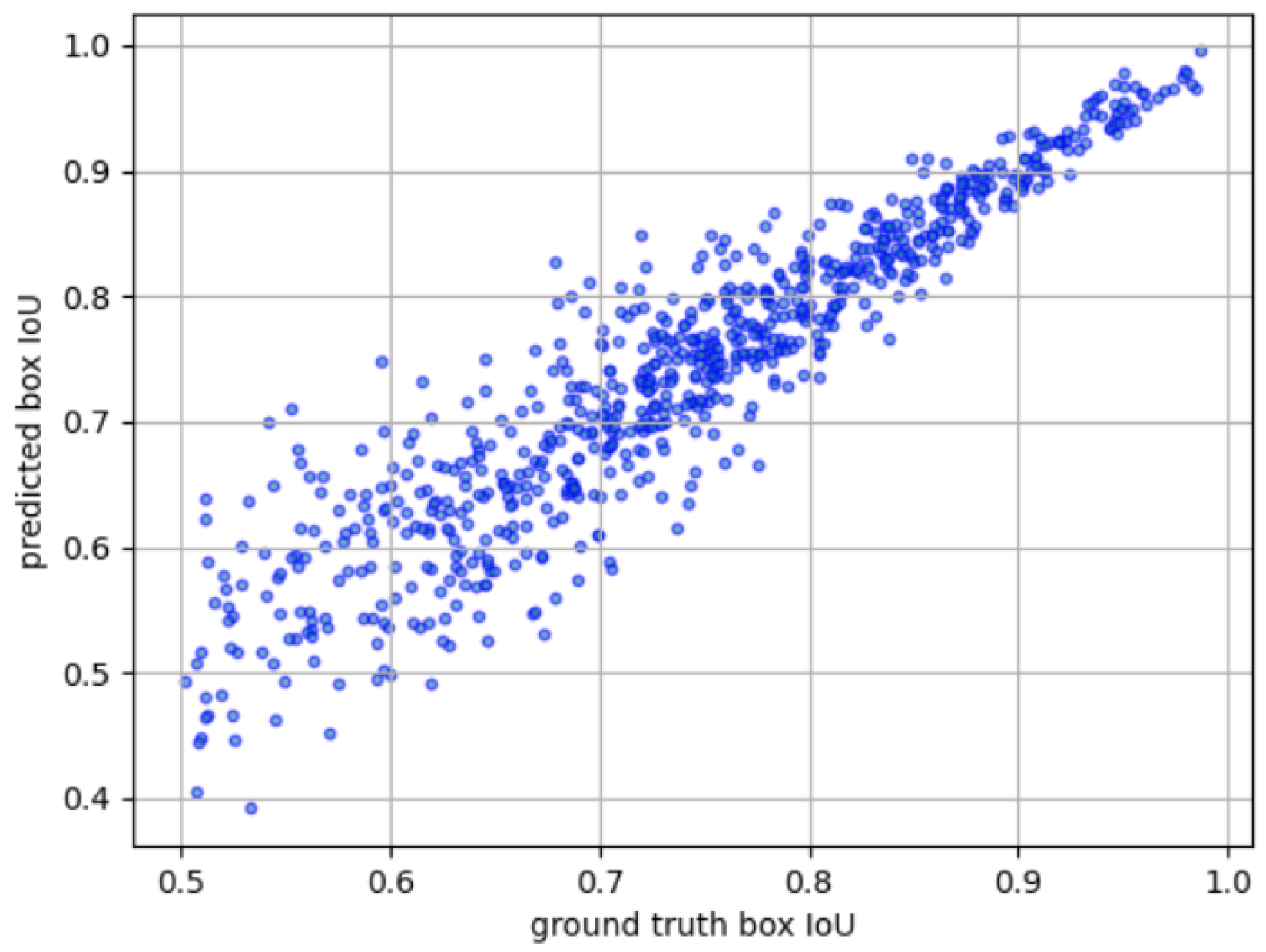
3.1.2. boxIoU Head
3.1.3. Training Loss
3.1.4. Inference
3.2. Active Learning with M-B Scoring R-CNN
3.2.1. Triplets-Based Active Learning Method
3.2.2. Balanced Sampling
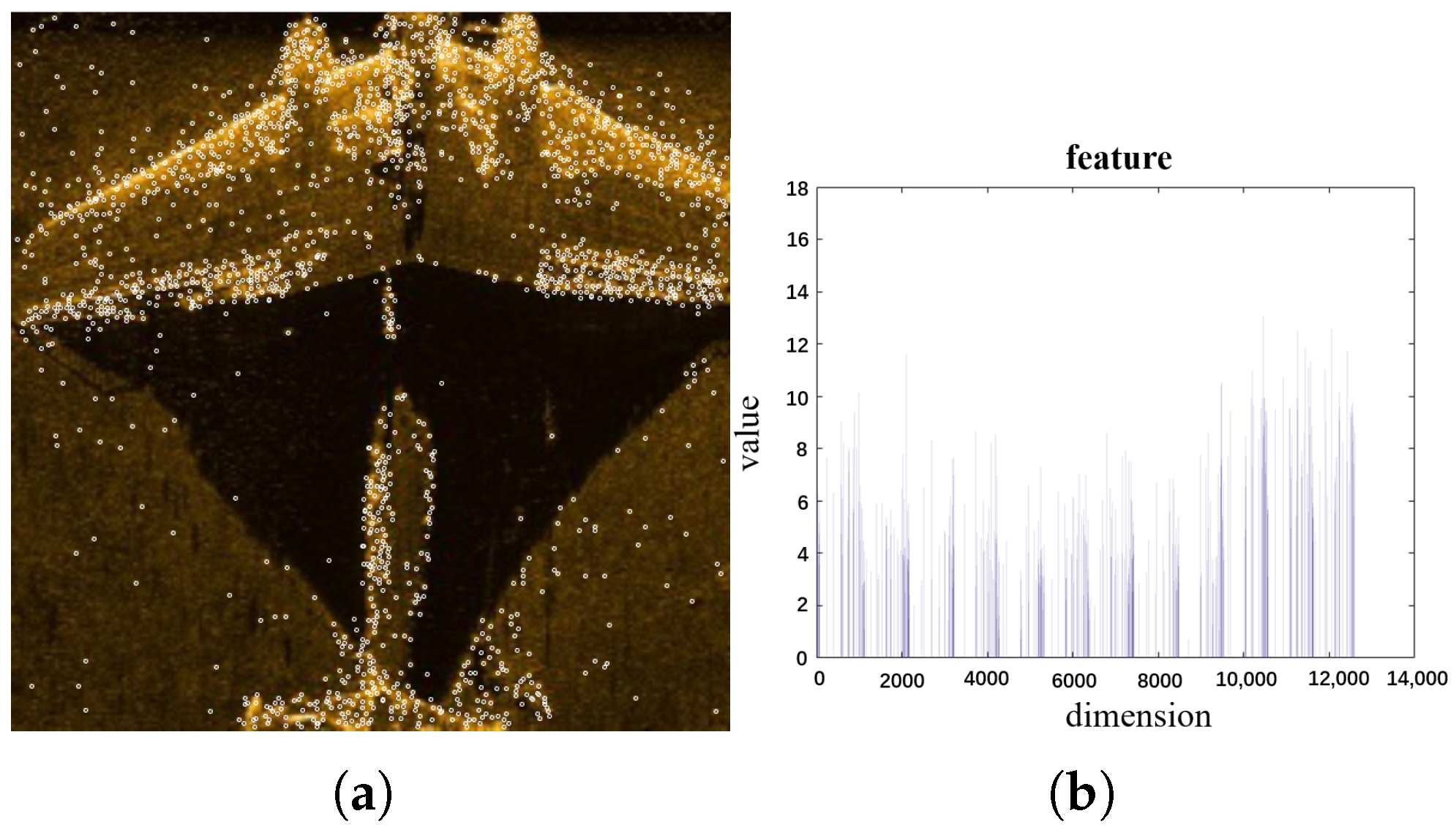
3.2.3. SIFT and Sparse Max Pooling Encoding
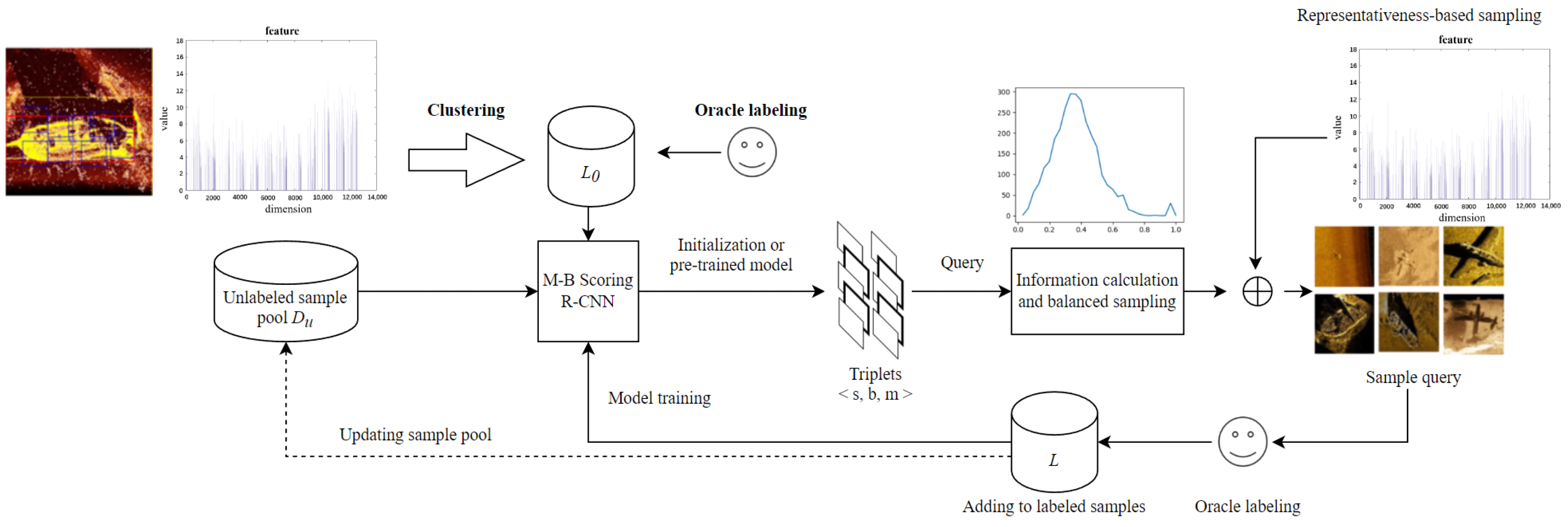
3.2.4. Deep Active Learning Framework
4. Experiments and Results
4.1. Sonar Image Dataset
4.2. Training Details
4.3. M-B Scoring R-CNN Results
4.4. TBAL and Balanced Sampling Results
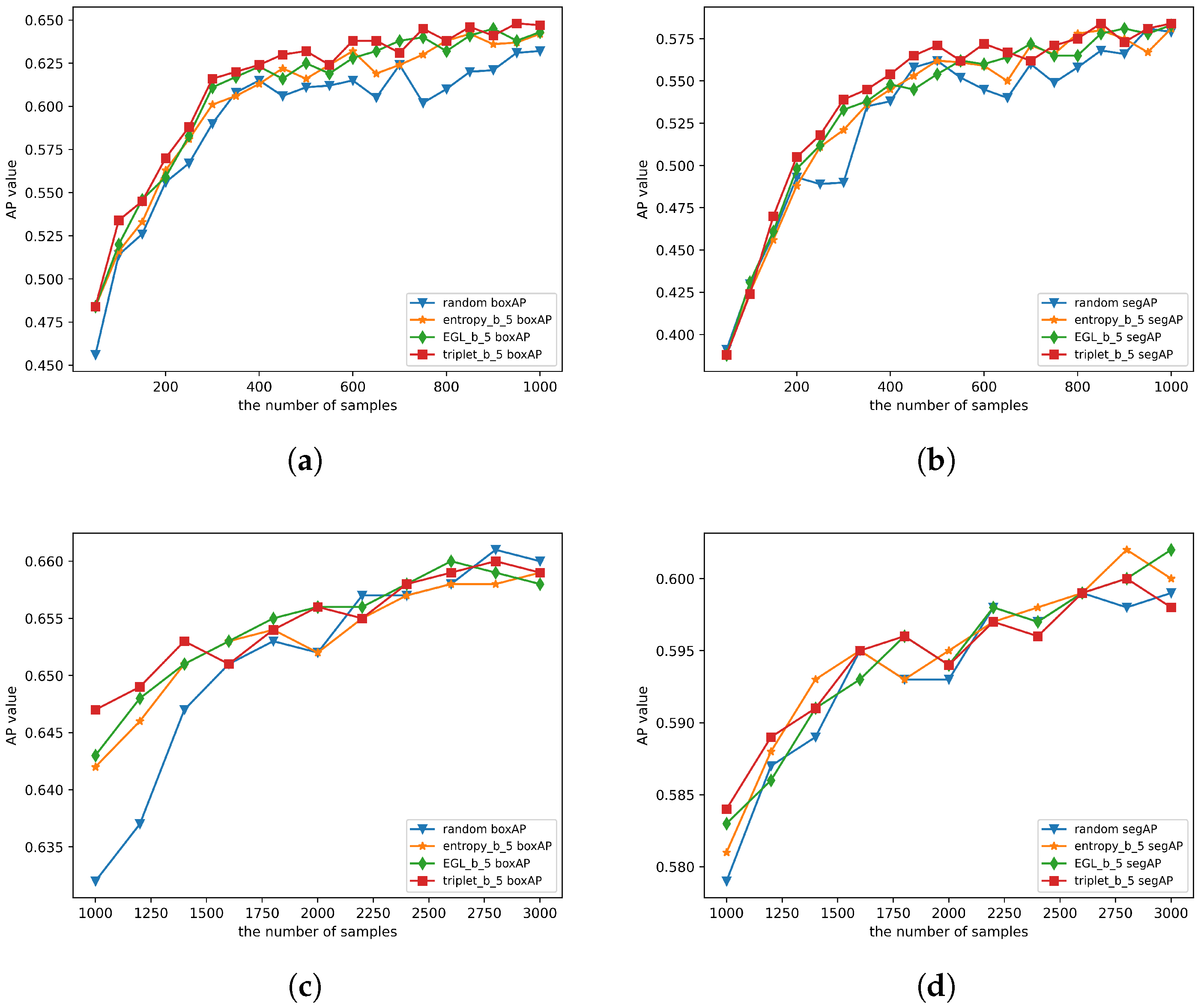
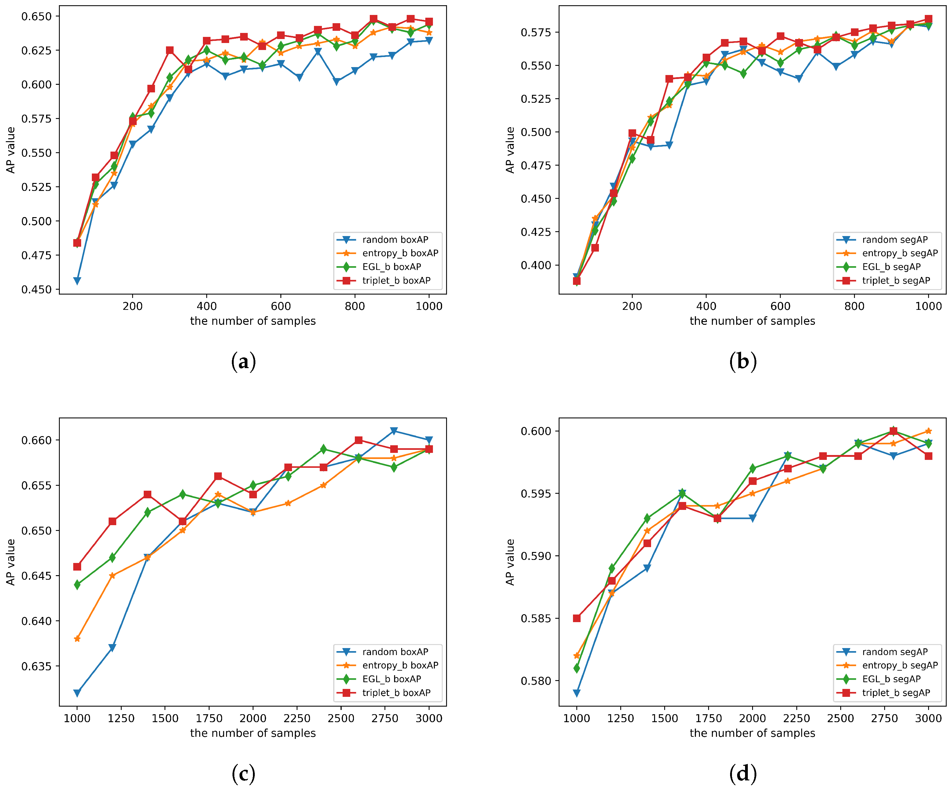
4.4.1. Verifying the Effectiveness of the TBAL Method
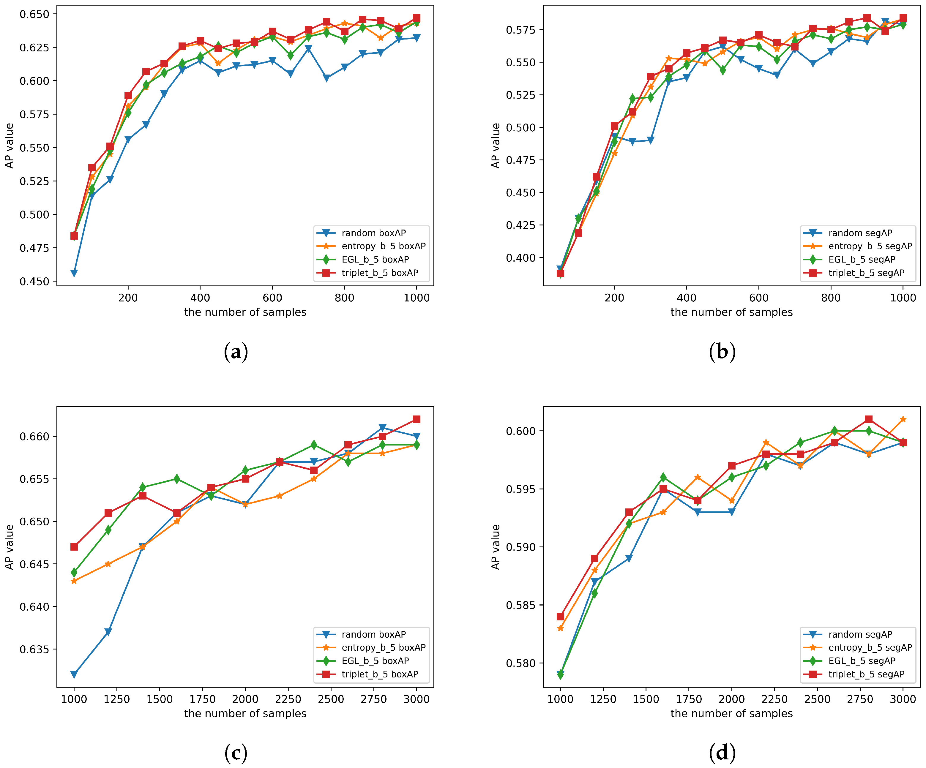
4.4.2. Verifying the Effectiveness of the Balanced Sampling Algorithm
4.4.3. Performance with Different Balance Factors
5. Conclusions
Author Contributions
Funding
Data Availability Statement
Conflicts of Interest
References
- Otsu, N. A threshold selection method from gray-level histograms. IEEE Trans. Syst. Man Cybern. 1979, 9, 62–66. [Google Scholar] [CrossRef] [Green Version]
- Torre, V.; Poggio, T.A. On edge detection. IEEE Trans. Pattern Anal. Mach. Intell. 1986, 8, 147–163. [Google Scholar] [CrossRef] [PubMed]
- Krizhevsky, A.; Sutskever, I.; Hinton, G.E. Imagenet classification with deep convolutional neural networks. Adv. Neural Inf. Process. Syst. 2012, 25, 1097–1105. [Google Scholar] [CrossRef]
- He, K.; Zhang, X.; Ren, S.; Sun, J. Deep residual learning for image recognition. In Proceedings of the IEEE Conference on Computer Vision and Pattern Recognition, Las Vegas, NV, USA, 27–30 June 2016; pp. 770–778. [Google Scholar]
- Girshick, R.; Donahue, J.; Darrell, T.; Malik, J. Rich feature hierarchies for accurate object detection and semantic segmentation. In Proceedings of the IEEE Conference on Computer Vision and Pattern Recognition, Columbus, OH, USA, 23–28 June 2014; pp. 580–587. [Google Scholar]
- Ren, S.; He, K.; Girshick, R.; Sun, J. Faster r-cnn: Towards real-time object detection with region proposal networks. Adv. Neural Inf. Process. Syst. 2015, 28, 91–99. [Google Scholar] [CrossRef] [PubMed] [Green Version]
- Liu, W.; Anguelov, D.; Erhan, D.; Szegedy, C.; Reed, S.; Fu, C.Y.; Berg, A.C. Ssd: Single shot multibox detector. In Proceedings of the European Conference on Computer Vision, Munich, Germany, 8–14 September 2016; Springer: Berlin/Heidelberg, Germany, 2016; pp. 21–37. [Google Scholar]
- Redmon, J.; Divvala, S.; Girshick, R.; Farhadi, A. You only look once: Unified, real-time object detection. In Proceedings of the IEEE Conference on Computer Vision and Pattern Recognition, Las Vegas, NV, USA, 27–30 June 2016; pp. 779–788. [Google Scholar]
- Chen, L.C.; Papandreou, G.; Kokkinos, I.; Murphy, K.; Yuille, A.L. Semantic image segmentation with deep convolutional nets and fully connected crfs. arXiv 2014, arXiv:1412.7062. [Google Scholar]
- Long, J.; Shelhamer, E.; Darrell, T. Fully convolutional networks for semantic segmentation. In Proceedings of the IEEE Conference on Computer Vision and Pattern Recognition, Boston, MA, USA, 7–12 June 2015; pp. 3431–3440. [Google Scholar]
- Chen, L.C.; Papandreou, G.; Kokkinos, I.; Murphy, K.; Yuille, A.L. Deeplab: Semantic image segmentation with deep convolutional nets, atrous convolution, and fully connected crfs. IEEE Trans. Pattern Anal. Mach. Intell. 2017, 40, 834–848. [Google Scholar] [CrossRef] [Green Version]
- Mozaffari, M.H.; Lee, W.S. Semantic Segmentation with Peripheral Vision. In Proceedings of the International Symposium on Visual Computing, San Diego, CA, USA, 5–7 October 2020; Springer: Cham, Switzerland, 2020; pp. 421–429. [Google Scholar]
- Mozaffari, M.H.; Lee, W.S. Dilated convolutional neural network for Tongue Segmentation in Real-time Ultrasound Video Data. In Proceedings of the 2021 IEEE International Conference on Bioinformatics and Biomedicine (BIBM), Houston, TX, USA, 9–12 December 2021; IEEE: Piscataway, NJ, USA, 2021; pp. 1765–1772. [Google Scholar]
- He, K.; Gkioxari, G.; Dollár, P.; Girshick, R. Mask r-cnn. In Proceedings of the IEEE International Conference on Computer Vision, Venice, Italy, 22–29 October 2017; pp. 2961–2969. [Google Scholar]
- Bolya, D.; Zhou, C.; Xiao, F.; Lee, Y.J. Yolact: Real-time instance segmentation. In Proceedings of the IEEE/CVF International Conference on Computer Vision, Seoul, Korea, 27–28 October 2019; pp. 9157–9166. [Google Scholar]
- Bai, M.; Urtasun, R. Deep watershed transform for instance segmentation. In Proceedings of the IEEE Conference on Computer Vision and Pattern Recognition, Honolulu, HI, USA, 21–26 July 2017; pp. 5221–5229. [Google Scholar]
- Kirillov, A.; Levinkov, E.; Andres, B.; Savchynskyy, B.; Rother, C. Instancecut: From edges to instances with multicut. In Proceedings of the IEEE Conference on Computer Vision and Pattern Recognition, Honolulu, HI, USA, 21–26 July 2017; pp. 5008–5017. [Google Scholar]
- Arnab, A.; Torr, P.H. Pixelwise instance segmentation with a dynamically instantiated network. In Proceedings of the IEEE Conference on Computer Vision and Pattern Recognition, Honolulu, HI, USA, 21–26 July 2017; pp. 441–450. [Google Scholar]
- Settles, B. Active Learning Literature Survey. In Computer Sciences Technical Report 1648; University of Wisconsin: Madison, NJ, USA, 2009. [Google Scholar]
- Gal, Y.; Islam, R.; Ghahramani, Z. Deep bayesian active learning with image data. In Proceedings of the International Conference on Machine Learning, Sydney, Australia, 6–11 August 2017; pp. 1183–1192. [Google Scholar]
- Sener, O.; Savarese, S. Active learning for convolutional neural networks: A core-set approach. arXiv 2017, arXiv:1708.00489. [Google Scholar]
- Yang, L.; Zhang, Y.; Chen, J.; Zhang, S.; Chen, D.Z. Suggestive annotation: A deep active learning framework for biomedical image segmentation. In Proceedings of the International Conference on Medical Image Computing and Computer-Assisted Intervention, Quebec City, QC, Canada, 11–13 September 2017; Springer: Berlin/Heidelberg, Germany, 2017; pp. 399–407. [Google Scholar]
- Jain, S.D.; Grauman, K. Active image segmentation propagation. In Proceedings of the IEEE Conference on Computer Vision and Pattern Recognition, Las Vegas, NV, USA, 27–30 June 2016; pp. 2864–2873. [Google Scholar]
- Huang, Z.; Huang, L.; Gong, Y.; Huang, C.; Wang, X. Mask scoring r-cnn. In Proceedings of the IEEE/CVF Conference on Computer Vision and Pattern Recognition, Long Beach, CA, USA, 15–20 June 2019; pp. 6409–6418. [Google Scholar]
- Zhao, Y.; Shi, Z.; Zhang, J.; Chen, D.; Gu, L. A novel active learning framework for classification: Using weighted rank aggregation to achieve multiple query criteria. Pattern Recognit. 2019, 93, 581–602. [Google Scholar] [CrossRef] [Green Version]
- Lewis, D.D.; Gale, W.A. A sequential algorithm for training text classifiers. In Proceedings of the SIGIR’94, Dublin, Ireland, 3–6 July 1994; Springer: Berlin/Heidelberg, Germany, 1994; pp. 3–12. [Google Scholar]
- Shannon, C.E. A mathematical theory of communication. Bell Syst. Tech. J. 1948, 27, 379–423. [Google Scholar] [CrossRef] [Green Version]
- Settles, B.; Craven, M.; Ray, S. Multiple-instance active learning. Adv. Neural Inf. Process. Syst. 2007, 20, 1289–1296. [Google Scholar]
- Nguyen, H.T.; Smeulders, A. Active learning using pre-clustering. In Proceedings of the Twenty-First International Conference on Machine Learning, Banff, AB, Canada, 4–8 July 2004; p. 79. [Google Scholar]
- Liu, Y.; Wang, Y.; Sowmya, A. Batch mode active learning for object detection based on maximum mean discrepancy. In Proceedings of the 2015 International Conference on Digital Image Computing: Techniques and Applications (DICTA), Adelaide, Australia, 23–25 November 2015; IEEE: Piscataway, NJ, USA, 2015; pp. 1–7. [Google Scholar]
- Bodla, N.; Singh, B.; Chellappa, R.; Davis, L.S. Soft-NMS–improving object detection with one line of code. In Proceedings of the IEEE International Conference on Computer Vision, Venice, Italy, 22–29 October 2017; pp. 5561–5569. [Google Scholar]
- Lowe, D.G. Object recognition from local scale-invariant features. In Proceedings of the Seventh IEEE International Conference on Computer Vision, Corfu, Greece, 20–27 September 1999; IEEE: Piscataway, NJ, USA, 1999; Volume 2, pp. 1150–1157. [Google Scholar]
- Lin, T.Y.; Maire, M.; Belongie, S.; Hays, J.; Perona, P.; Ramanan, D.; Dollár, P.; Zitnick, C.L. Microsoft coco: Common objects in context. In Proceedings of the European Conference on Computer Vision, Zurich, Switzerland, 6–12 September 2014; Springer: Berlin/Heidelberg, Germany, 2014; pp. 740–755. [Google Scholar]


| Dataset Type | Corpse | Shipwreck | Planewreck |
|---|---|---|---|
| Training Set | 1014 | 1078 | 1066 |
| Test Set | 376 | 386 | 400 |
| Method | Backbone | boxAP | boxAP50 | boxAP75 | segAP | segAP50 | segAP75 |
|---|---|---|---|---|---|---|---|
| M-BS R-CNN | ResNet-50 | 0.660 | 0.986 | 0.817 | 0.599 | 0.980 | 0.705 |
| MS R-CNN | ResNet-50 | 0.650 | 0.986 | 0.806 | 0.598 | 0.982 | 0.703 |
| Mask R-CNN | ResNet-50 | 0.647 | 0.983 | 0.796 | 0.586 | 0.979 | 0.676 |
| M-BS R-CNN | ResNet-101 | 0.672 | 0.987 | 0.844 | 0.602 | 0.982 | 0.713 |
| MS R-CNN | ResNet-101 | 0.661 | 0.986 | 0.823 | 0.603 | 0.982 | 0.713 |
| Mask R-CNN | ResNet-101 | 0.656 | 0.985 | 0.811 | 0.593 | 0.979 | 0.699 |
Publisher’s Note: MDPI stays neutral with regard to jurisdictional claims in published maps and institutional affiliations. |
© 2022 by the authors. Licensee MDPI, Basel, Switzerland. This article is an open access article distributed under the terms and conditions of the Creative Commons Attribution (CC BY) license (https://creativecommons.org/licenses/by/4.0/).
Share and Cite
Xu, F.; Huang, J.; Wu, J.; Jiang, L. Active Mask-Box Scoring R-CNN for Sonar Image Instance Segmentation. Electronics 2022, 11, 2048. https://doi.org/10.3390/electronics11132048
Xu F, Huang J, Wu J, Jiang L. Active Mask-Box Scoring R-CNN for Sonar Image Instance Segmentation. Electronics. 2022; 11(13):2048. https://doi.org/10.3390/electronics11132048
Chicago/Turabian StyleXu, Fangjin, Jianxing Huang, Jie Wu, and Longyu Jiang. 2022. "Active Mask-Box Scoring R-CNN for Sonar Image Instance Segmentation" Electronics 11, no. 13: 2048. https://doi.org/10.3390/electronics11132048
APA StyleXu, F., Huang, J., Wu, J., & Jiang, L. (2022). Active Mask-Box Scoring R-CNN for Sonar Image Instance Segmentation. Electronics, 11(13), 2048. https://doi.org/10.3390/electronics11132048