1. Introduction
Vision-threatening ocular diseases (ODs), such as age-related macular degeneration (AMD), diabetic retinopathy (DR), cataracts, uncorrected refractive errors, and trachoma, have become remarkably common over the past two decades. A recent world report on vision from the World Health Organization (WHO) demonstrated that visually impaired persons worldwide exceed 2.2 billion. At least
of these cases could have been prevented or are yet to be addressed [
1]. Trachoma, cataracts, and uncorrected refractive errors (e.g., myopia, astigmatism, hypermetropia, and presbyopia) are three leading causes of blindness and vision impairment. According to the WHO, more than 153 million people are visually impaired due to uncorrected refractive errors, almost 18 million people are bilaterally blind from cataracts, and approximately
million are diagnosed with trachoma [
2]. Moreover, studies showed that AMD is the most common cause of blindness, particularly in developed countries, as it accounts for
(i.e., 3 million people) of all blindness worldwide. The number of cases is expected to increase to 10 million by 2040 [
1,
3]. Recent studies [
4,
5] also showed that out of the 37 million cases of blindness worldwide,
of cases are due to DR (i.e., 1.8 million persons). According to the WHO [
6], more than 171 million people globally had diabetes in 2000. This number is projected to rise to 366 million by the year 2030. Nearly half of patients who have diabetes are unaware of their condition. About
of persons with diabetes become blind, and about
develop severe visual loss after 15 years. Moreover, more than
of patients will have some form of DR after 20 years of having diabetes. Thus, early diagnosis and timely treatment of ODs are vital to prevent irreversible vision loss. Ocular fundus imaging [
7] is commonly utilized as an effective and economical tool for screening retina disorders and monitoring disease progression in ophthalmology. Compared to in-person ophthalmologist examination, retinal photography has high sensitivity, specificity, and inter-/intra-examination agreement. Thereby, retinal photographs can be used in place of ophthalmoscopy in many clinical situations. Advances in optical fundus imaging have made it easier to obtain high-quality retinal images, even without pupillary dilation. Fundus cameras offer several advantages. They are convenient for patients because of the single flash exposition of the floodlight. Moreover, they do not affect the image quality in different situations, such as a degradation reduction in cataract cases. In general, digital retinal photography can facilitate telemedical consultation, which provides increased access to accurate and timely sub-specialty care, particularly for under-served areas.
However, there are several challenges associated with diagnosing ocular diseases. First, common ODs, such as DR, cataracts, and AMD, progress with few initial visible symptoms, making it difficult to achieve precise diagnoses in the early stages [
8]. Second, physicians may need a long time to diagnose the patient’s condition. Third, the diagnosis needs experts who are not available all the time. Fourth, despite the merits offered by ocular fundus imaging, it is sometimes difficult to obtain sufficient accurate fundus images, especially for some rare fundus diseases [
9]. This is primarily because the produced fundus images have a minimal contrast and might contain features similar to eye anatomies, making it challenging to differentiate between them [
10]. As a result, all signs of eye diseases might not be precisely discovered by an ophthalmologist. Thus, an accurate diagnosis of the exact disease grade would be challenging. To address the above-mentioned challenges, several computer-aided diagnosis (CAD) systems have been proposed to automate the process of OD detection [
11]. Machine learning techniques have been widely employed for ocular disease diagnosis in such CAD systems [
12]. Ocular diagnosis systems based on conventional classifiers, such as support vector machines (SVM) [
13] and K-nearest neighbor (KNN) [
14], demonstrated good performance for small datasets but work unwell in large-scale datasets. Thus, such methods might not suit OD detection, which is more challenging and specific. Moreover, conventional machine learning techniques require manual feature extraction, feature selection, and classification.
Deep learning (DL) has recently become the mainstream technology in computer vision. It has received extensive research interest in developing new medical image processing algorithms to support disease detection and diagnosis [
15,
16,
17,
18,
19,
20,
21]. Compared to conventional machine learning technologies, DL methods avoid lesion segmentation and handcrafted feature identification and computation. These tasks, especially in retinal fundus images, burden the developer because of the previously mentioned problems. Thus, utilizing DL can develop CAD systems schemes more efficiently. Convolutional neural networks (CNN) have achieved revolutionizing success in fundamental computer vision and image processing problems, including classification and segmentation [
22]. Highly discriminative features can be learned from raw pixel intensities using CNNs [
23]. The first layers of a CNN can extract edges at particular locations and orientations in the image. The middle layers can detect structures composed of particular arrangements of edges. More complex structures that correspond to parts of familiar objects can be detected using the last layers [
24].
Several different ODs can co-occur in the human eye. Therefore, a model needs to be optimized to diagnose the various ODs types based on multi-label classification (ML-C). ML-C means that each training example is associated with more than one label [
25]. Prediction of a single label is the goal of typical classification tasks. However, it might be required to predict the likelihood across several class labels at the same time where the classes are generally assumed to be mutually exclusive. In ML-C, it is necessary to simultaneously output zero or more labels for each input sample [
26]. Many studies were conducted to detect the various ODs, but a few utilized ML-C of the ODs as one patient can have more than one type of eye disease. Therefore, optimizing the models that support the concept of ML-C is very important. On the other hand, many studies merely apply the existing universal models in classifying ODs rather than building new or optimizing current architectures. That lessens the classification accuracy because the model can perform accurately in one field while it cannot be applied to the other.
This paper presents a novel CAD system for detecting various ODs using ML-C. We utilize a multi-label (ML) benchmark dataset, the retinal fundus multi-disease image dataset (RFMiD) [
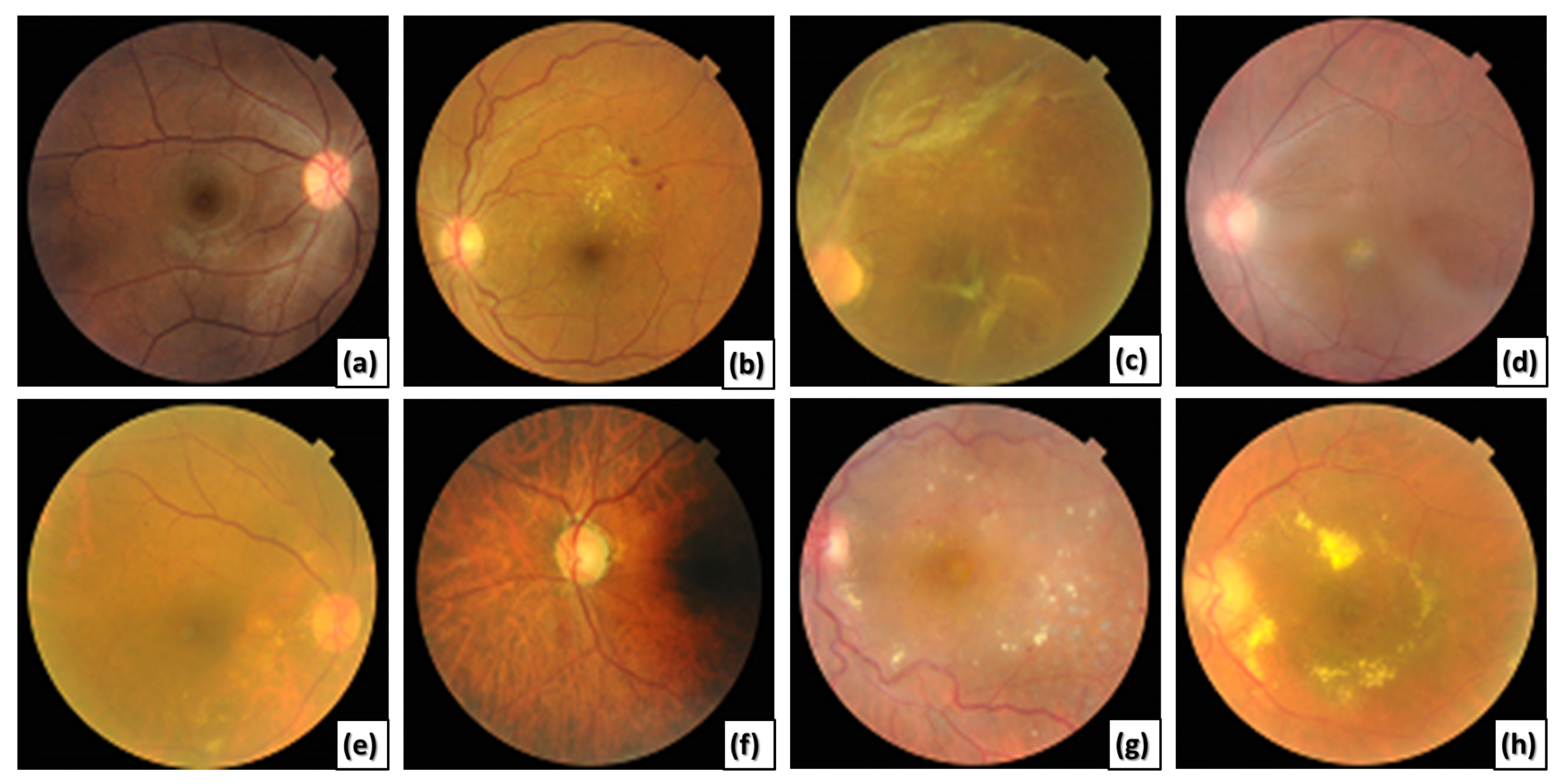
27], that contains 45 classes of fundus retinal images. Most of the images in the utilized dataset may include more than one disease simultaneously, as shown in
Figure 1.
Table 1 clarifies the different ODs shown in
Figure 1, along with their labels and definitions. The proposed CAD system starts with preprocessing steps that include the normalization and augmentation by some transformation processes. After that, we train the divided data using our proposed CNN model. Then, we test the unknown images from different diseases. The results of the proposed CAD system are probabilities of the ODs. We utilize different evaluation metrics and compare the proposed system with various state-of-the-art schemes to demonstrate its efficiency and reliability. The main contributions of this work are summarized in the following points:
We propose an ML-CAD framework based on DL for simultaneous diagnosis of interleaved ODs from color fundus images.
The effectiveness of the proposed framework is verified utilizing a recent publicly available ML dataset (RFMiD) that contains a wide variety of challenging ocular diseases.
We compare the performance of the proposed framework, utilizing five different measures, with similar frameworks and built-in models. The experimental results illustrate the practicality and superiority of the proposed framework.
Compared to existing multiple ocular diseases frameworks that can detect at most ten ODs, the proposed framework can detect more than twenty-nine ODs.
The rest of this paper is organized into five sections.
Section 2 presents the related works. It discusses the current limitations and highlights the main directions and solutions included in the proposed system to overcome the current shortcomings.
Section 3 explains the detailed phases and techniques utilized in the proposed CAD framework.
Section 4 describes the different experiments conducted and presents the findings.
Section 5 introduces the discussion and provides a comparative analytical study of the proposed CAD system and other state-of-the-art techniques. Finally,
Section 6 presents the conclusion of the work and findings and highlights future research directions.
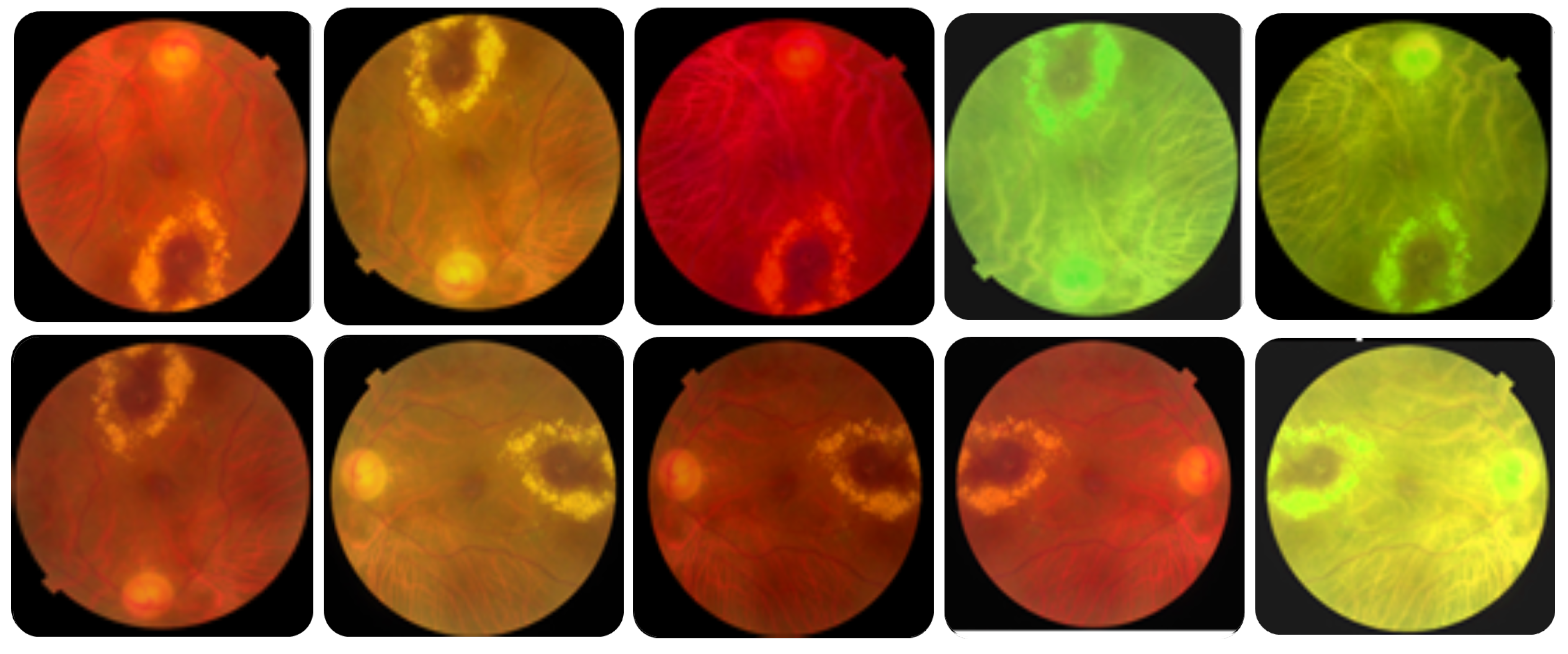
Figure 1.
Different retinal color fundus images with different ODs. (a) Normal, (b) DR, (c) RT, (d) MH and MS, (e) MH and DN, (f) MH, MYA, and ODC, (g) DR, LS, and TV, and (h) EDN, ODP, and TSLN.
Figure 1.
Different retinal color fundus images with different ODs. (a) Normal, (b) DR, (c) RT, (d) MH and MS, (e) MH and DN, (f) MH, MYA, and ODC, (g) DR, LS, and TV, and (h) EDN, ODP, and TSLN.
Table 1.
Different ODs with their labels, definitions, and indicators.
Table 1.
Different ODs with their labels, definitions, and indicators.
| ODs | Label | Definition | Indicators |
|---|
| Diabetic Retinopathy [28] | DR | A microvascular complication of diabetes mellitus caused by high blood sugar levels damaging the back of the eye (retina). | Microaneurysms, retinal dot and blot hemorrhage, hard exudates, or cotton wool spots. |
| Age-related Macular Degeneration [29] | AMD | Known as macular degeneration and is caused by deterioration of the macula. | Multiple drusen in the macular region, geographic atrophy involving the fovea. |
| Media Haze [30] | MH | The opacity of media. | Cataracts, vitreous opacities, corneal edema, or small pupils. |
| Retinitis [31] | RS | It is inflammation of the retina. | Numerous microbes cause it. Vitreous inflammation, macular star, intraretinal hemorrhage, phlebitis, arteritis, and hyperemic disc. |
| Macular Scar [32] | MS | A scar at the central part of the retina. | The macular pucker separates from the retina. |
| Retinal Traction [33] | RT | The separation of the neurosensory retina from the underlying retinal pigment epithelium (RPE) due to the traction resulting from membranes in the vitreous or over the retinal surface. | Retinal ischemia and atrophy of the photoreceptor layer: neovascularization of iris (NVI), neovascularization of angle (NVA), and neovascular glaucoma (NVG). |
| Exudation [27] | EDN | Represented as a circle of exudates surrounding the macular area. | The hard exudates are white or yellowish lipid deposits with sharp edges. |
| Drusens [34] | DN | Yellow deposits under the retina. They are made up of lipids and proteins. Drusens likely do not cause ARMD, but they may be a sign of ARMD. | Tiny pebbles of debris that build up over time. |
| Myopia [35] | MYA | Objects in the distance appear blurred while close objects are often seen clearly. | Degenerative changes in the choroid, sclera. The eye is too long or the cornea is more curved. |
| Optic Disc Cupping [36] | ODC | The thinning of the neuroretinal rim such that the optic disc appears excavated. It is usually identified with glaucoma. | Congenital optic disc anomalies, ischaemic, hereditary, and traumatic optic neuropathies, or in situations in which the anterior visual pathway is compromised, such as intracranial aneurysms or tumors. |
| Laser Scars [27] | LS | Laser therapy treatment to stop the progression of vascular leaks. | Circular or irregularly shaped scars on the retinal surface. |
| Tortuous Vessels [27] | TV | Related to hypertension and diabetes. | Tortuosity of the retinal blood vessels. |
| Optic Disc Pallor [37] | ODP | The anatomic sequelae of atrophy of the anterior visual pathway with the loss of retinal ganglion cells. | Pale yellow discoloration of the optic disc and absence of many small vessels. |
| Tessellation [38] | TSLN | A common characteristic of myopic eyes and a clinical marker for the development of retinochoroidal changes. | It appears due to the thinning of RPE and choriocapillaris. The choroidal vessels are visible due to the reduced density of the pigments. |
2. Related Work
This section reviews the existing diagnosis systems for ODs. We discuss the current limitations and highlight the main directions and remedies suggested in the proposed system to overcome the current shortcomings. For example, He et al. [
8] presented a CAD system using a dense correlated network (DCNet) to classify color fundus images. They used a public dataset (ODIR 2019) based on seven types of ODs using ML-C. The authors utilized two fully connected layers with rectified linear unit (ReLU) activation in one of them. One dense layer is 512, and the other is 8 as the number of the output categories of the ODs. They employed an ML soft margin loss function. The main advantage of their method is that it can be used in multi-modal image analysis. However, they could not compare their model with other existing works because their method is patient-based, and the other studies are image-based. They shared the same backbone CNN to extract features from the right and left eyes to reduce the computation complexity. Hence, they could not handle the unbalanced distribution of patient cases.
Wang et al. [
9] utilized transfer learning to extract features of the color fundus images and then utilized ML-C based on problem transformation. The authors utilized a multi-label dataset with eight labels. They utilized histogram equalization on gray and colored images. Then, they applied two classification models to the two images sets. Finally, they obtained the average of the sigmoid output probabilities from the two models. The main limitation of their work is the low network performance because of the variety of uncommon ODs categorized in the label “other diseases” in the utilized dataset. In addition, their system suffers from the data imbalance problem due to the limited data in some disease categories. Hence, some of the specific features learned are unknown.
Cheng et al. [
39] used a graphical convolution network (GCN) to detect eight DR lesions (laser scars, drusen, cup disc ratio, hemorrhages, retinal arteriosclerosis, microaneurysms, hard and soft exudates) from color fundus images. They utilized ResNet-101, then two convolutional (CONV) layers with a
kernel, stride 2, and adaptive max pooling for feature extraction. Their model’s accuracy (ACC) and receiver operating characteristic (ROC) values showed better detection results for laser scars, drusen, and hemorrhage lesions. In contrast, their system had poor detection ability for microaneurysms, soft exudates, and hard exudates. This is mainly because microaneurysms appeared as small red spots in the retinal capillaries. Thus, the model could not distinguish microaneurysms from the background of the fundus images. On the other hand, soft and hard exudate lesions often accompanied multiple other fundus lesions simultaneously, which made it difficult for the model to extract the features of all fundus lesions.
Dipu et al. [
40] utilized transfer learning to detect eight ODs from the ODIR2019 dataset. They compared the performance of some state-of-the-art DL networks, such as Resnet-34, EfficientNet, MobileNetV2, and VGG-16. The authors trained the cutting-edge on the utilized dataset and reported the results. They evaluated the models’ performance by estimating the ACC. They ordered the models due to the resulting ACC into VGG-16, Resnet-34, MobileNetV2, and EfficientNet. However, the authors did not build a new model to detect the ODs. Moreover, calculating only ACC was not enough to estimate the model performance.
Choi et al. [
41] proposed a CAD system using random forest transfer learning based on VGG-19. They utilized a small dataset in order to detect ten OD categories. They observed that the ACC increases by decreasing the classes that need to be detected to three. On the contrary, when they increased the categories to ten, the ACC decreased with a difference of about
. The authors tried to use an ensemble classifier with transfer learning and found a slight increase in ACC of
. Although the authors made augmentation, they could not achieve good performance because of the data imbalance.
Diaz Pinto et al. [
23] utilized DL to detect glaucoma from color fundus images. First, they cropped the images around the optic disc. Then, other transformation processes were applied, such as random rotations, zooming by a range between 0 and 0.2, and horizontal and vertical flipping. They utilized VGG16, VGG19, InceptionV3, ResNet50, and Xception. Each architecture was followed by global average pooling. They used the softmax classifier. The authors used stochastic gradient descent (SGD) for updating weights. They set epochs to 100 and 250. The batch size was set to 8, the learning rate (LR) was set to
, and the momentum rate was 0.9. The fine-tuning performance was decreased when testing the CNNs on databases that were different from those used for training.
Tan et al. [
42] classified AMD by using a CNN. Their proposed model consists of seven CONVs with a
kernel, four max-pooling (MP) (
), and three fully connected (FC) layers. The proposed model was fully automatic so that no hand-crafted feature extraction or selection was required. Moreover, no classifier was required as they involved meticulous engineering in designing a feature extraction module that could extract highly distinctive features for classification. The proposed model can be installed in a cloud system. On the other hand, the authors highlighted the issues of their model, as the overall diagnostic performance of their CNN model was poor and would improve with more extensive data. Furthermore, the proposed model suffered from convergence and overfitting problems. In addition, the training of the CNN model was slow and intensive. A summary of the most recent studies (published from 2018 to 2021) is shown in
Table 2.
From the previous review of the current studies conducted recently, we can conclude their main limitations in diagnosing multiple ODs based on the ML-C concept as follows:
Increasing the number of classes decreases the model performance, mainly if the number of training samples is not sufficiently large;
Some systems are conservative and cannot be applied in the real world because of the imbalanced and/or insufficient datasets;
Some models suffer from overfitting;
The overall performance of the ML-C based models is minor compared to ML- or binary classification-based models because of overlapping labels.
To overcome the previous limitations, we propose a novel ML CAD system to accurately diagnose the different ODs from various ML color fundus images. We apply some augmentation processes to enlarge the training dataset and avoid overfitting and data imbalance issues. On the other hand, data augmentation improves the model performance. We utilize basic augmentation for preserving the labels after transformation. Moreover, we suggest a novel CNN model to extract feature maps (FM) of the augmented images. We customized the different hyper-parameters of the CONV layers, dense layers, dropout (DO), stride, kernel, filters, MP, optimizer, regularization, LR, loss function, number of epochs, batch size, and classifier to provide precise results. The proposed model can report the probability of each disease of the 45 ODs in each image. Finally, we evaluated the system performance using six different metrics and compared it with many current systems and models.
3. The Proposed ML CAD System
This section gives a detailed explanation of the proposed multiple OD ML-based CAD system. The proposed system consists of three phases. It starts by supplying the preprocessing phase with the ML dataset [
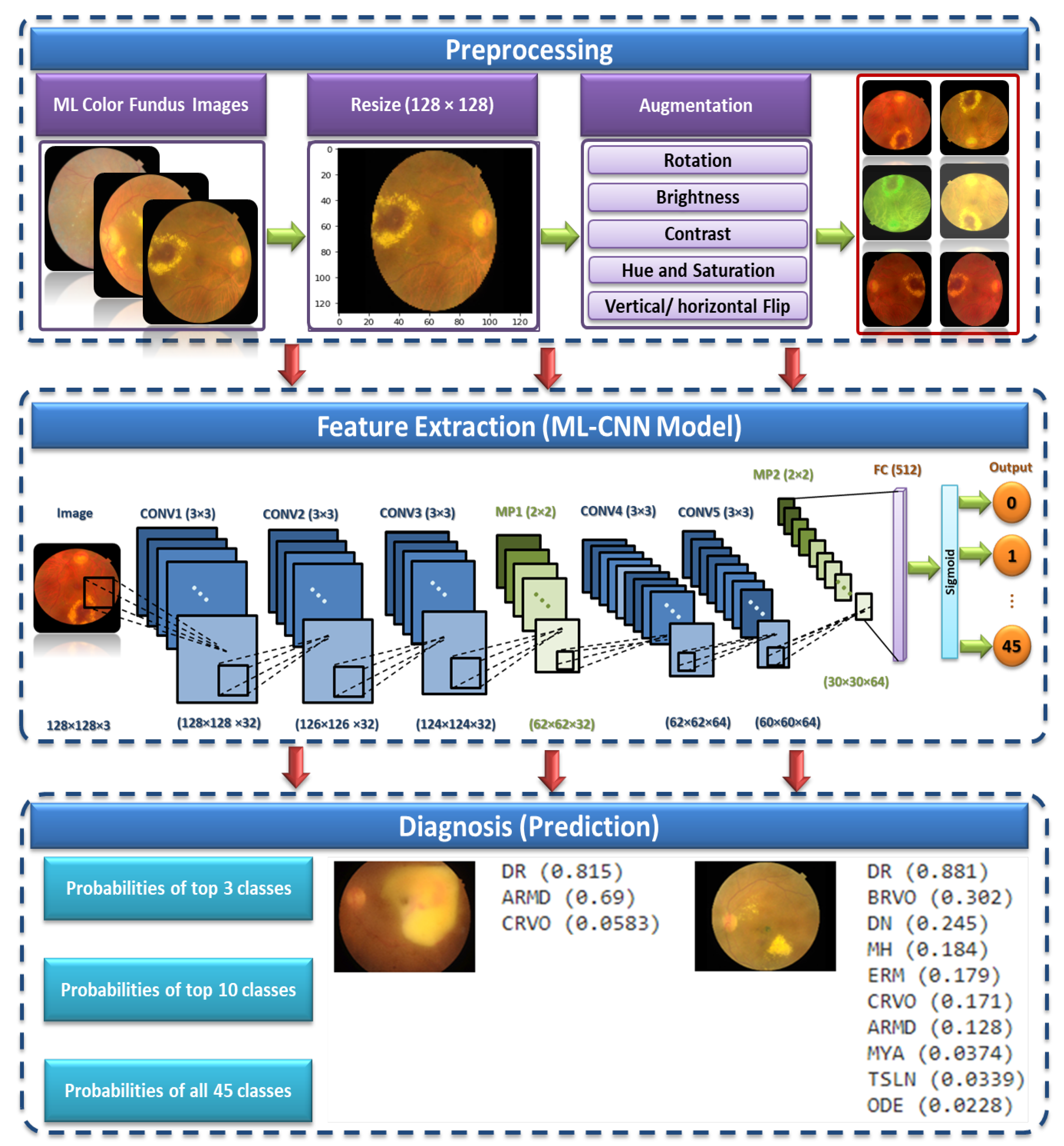
27]. This phase aims to scale the images to a standard size and apply some transformation processes, such as vertical and horizontal flipping, rotation, and brightness, contrast, hue, and saturation adjustments. The normalized preprocessed images are then fed to the proposed CNN model in the feature extraction and ML-C phase. Finally, the prediction is obtained by testing the proposed CNN model.
Figure 2 shows the proposed ML CAD system. We present below the three phases of the proposed system in detail.
3.1. Preprocessing
The preprocessing stage consists of two main phases, which are image resizing and data augmentation. These phases are discussed in the following subsections.
Image Resizing. All images are resized to a standard size of pixels. Although using the actual size could be helpful in learning, resizing the input images is essential to save memory and space and reduce the training time.
Data augmentation. Each image in the utilized dataset could contain multiple diseases out of forty-five different ODs. However, this dataset is imbalanced because the number of normal samples could greatly outnumber the samples of some abnormal classes (diseases). For instance, while the number of normal images (i.e., negative samples) in which no ODs appear in the training dataset is 401, the number of images in which some diseases appear, such as cotton-wool spots (CWS) and choroidal folds (CF), are less than 10. Thus, data augmentation methods should be utilized to increase the number of images in which rare diseases appear and reduce the positive-negative class imbalance.
Different transformation methods [
43] can be applied to the image dataset to enlarge the dataset, solve class imbalances, and avoid overfitting. In this work, we utilized simple, safe, and manageable augmentation methods to preserve labels and encourage the model to learn more general features. The safety of a data augmentation method refers to its likelihood of preserving the label post-transformation. Precisely, we used different augmentation methods, including horizontal and vertical flipping, rotation, brightness change, saturation change, and hue change, to images of rare diseases to ensure that each label in the dataset occurs at least 100 times.
Table 3 lists the utilized augmentation methods and the corresponding parameters’ values, and
Figure 3 shows an example of an augmented image to 10 images. The number of training samples increased from 1920 to 4784 after data augmentation.
3.2. Feature Extraction and ML-C
The CNN general architecture is made up of CONV, pooling (PO), and FC layers [
44,
45]. Each component may at least consist of one layer. Different mapping functions and regulatory units, such as batch normalization (BN) and DO, are also included in the architecture to optimize the performance and avoid overfitting. The CONV operation picks up distinct features from the input color fundus image. It is performed with kernel filters to generate feature maps (FMs). Some down-samplings are included in the architecture, such as stride and PO. A stride is the number of units the filter slides upon for CONV and MP. On the other hand, each successive FM would get smaller after the CONV process without zero paddings. At last, the CONV layer output is passed to a non-linear activation function (AF), such as sigmoid and ReLU.
Pooling [
46] regulates the CNN complexity and ensures the fixed size of the output. It decreases the learnable parameters and reduces FM size. Moreover, it increases the generalization and reduces overfitting. Pooling in CNNs can be MP or global pooling (GP), among other alternatives. The MP operation takes the highest value from each kernel. Finally, in FC (dense layer) [
47], the output of CONV and PO layers is flattened and transformed into a 1D array. The weight connects each input with each output. The output nodes have the same number of classes.
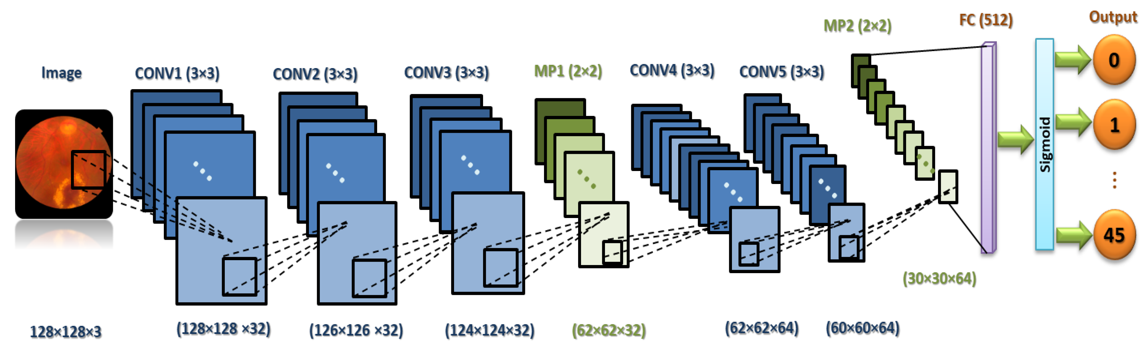
It is necessary to focus on the arrangement of all components in CNN architecture. This arrangement plays a vital role in building new architectures and achieving the needed performance. Therefore, the proposed ML-CNN model consists of three CONV layers with 32 filters and a kernel size of , and the AF is ReLU. Then, the MP layer with a kernal is performed, followed by DO with 0.25 for regularization. Again, two CONV layers with 64 filters are performed, followed by one MP () and DO with 0.25. After that, one flatten layer is performed, followed by one FC layer with 512 neurons. We add another DO with 0.5. Finally, one FC layer with 45 nodes is performed. The total trainable parameters are 29,589,613.
Figure 4 demonstrates in detail the layers of the proposed ML-CNN model, and
Table 4 shows the proposed ML-CNN architecture. The configurations of the hyper-parameters utilized in the proposed ML-CNN model are presented in
Table 5. The optimizer is the SGD with LR equal to 0.01, decay equal to
, and momentum rate equal to 0.9. The batch size is 32, the loss function is categorical cross-entropy, the AF of the final FC layer is sigmoid, and the number of epochs is 50.
We utilize the sigmoid function at the end of the ML-CNN model classifier to transform the raw output values into probabilities, which is the final understandable format. Moreover, the sigmoid function is suitable in the ML-C problem [
48] because since there is more than one “right answer”, the outputs are not mutually exclusive. The probabilities produced by the sigmoid function are independent and are not constrained to sum to one. In addition, the sigmoid function allows us to have a high probability for all OD classes, some of them or none. For example, when classifying ODs in the color fundus image, the image might contain DR and/or RS, or none of those defects.
3.3. The Prediction
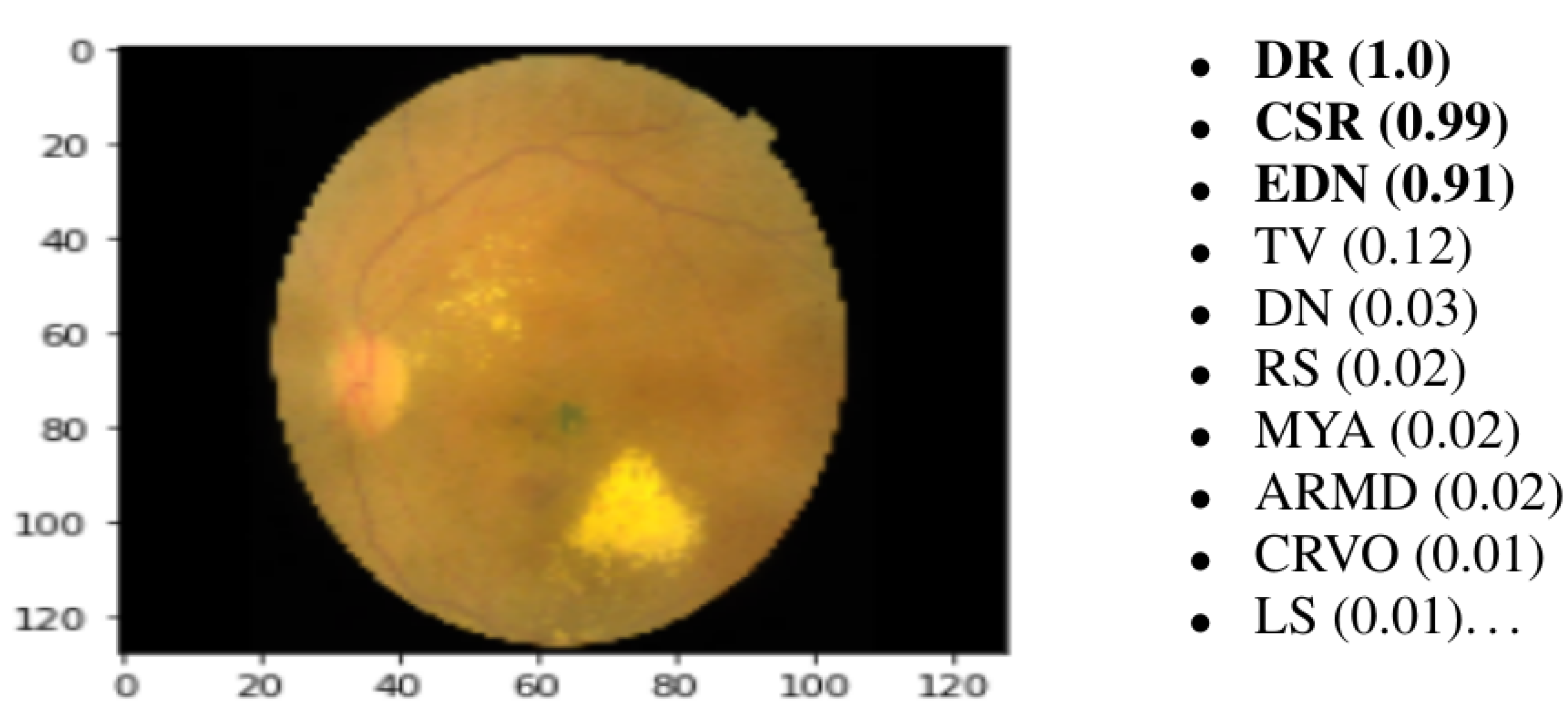
The last layer of the proposed model is a fully connected layer that consists of forty-five output neurons. The output of this layer provides the probabilities of the 45 ODs in the utilized RFMiD dataset. Based on the output probabilities, the model can predict whether each OD appears in the image presented to the model. For each label (disease), if the corresponding probability is larger than a preset cut-off value (0.50), our model confirms the presence of this disease in the presented image.
Figure 5 shows an example of an image presented to the proposed model along with the top 10 ODs with the highest probabilities. It can be observed that only the top three ODs are confirmed by the model based on the preset cut-off value.
The proposed model is validated using the 10-fold cross-validation technique to reduce overfitting. The training set is split into k (=10) smaller subsets. The proposed ML-CNN model is trained using of the folds as the training set of data, and the resulting model is validated on the remaining part of the data. The output of the model and validation using five different metrics for evaluating the performance of the proposed model are discussed in detail in the next section.
4. Experimental Results
This section gives a detailed description of the dataset and explains the utilized performance metrics. Finally, we present the results obtained from applying the proposed ML-CNN model.
RFMiD is an ML dataset where each image contains multiple ODs. It consists of 3200 images, including normal and abnormal cases (669 images are normal, and the rest are abnormal). The abnormal images include 45 diseases or classes in which DR appears in 632 images, MH appears in 523 images, and ODC appears in 445 images. The remaining diseases appear in smaller numbers of images. The full list of diseases and the number of images in which each disease appears is shown in
Table 6. In addition, the complete name of each disease can be found in [
27]. All images were captured with three fundus cameras, namely, TOPCON 3D OCT-2000, TOPCON TRC-NW300 with a distance of 40.7 mm and a
field of view (FOV), and Kowa VX-10 with a distance of 39 mm and a
FOV. The images are in various resolutions, such as
,
and
.
The utilized dataset contains a CSV file that includes the image ID, disease risk (presence of disease/abnormality), and 45 classes of ODs, which are found in the color fundus images. An image is assigned the value ‘0’, in the CSV sheet, if it does not have a specific disease (out of the 45 diseases) and labeled by ‘1’ otherwise. For instance, if the image includes DR, RS, and LS, but does not include the remaining ODs, only columns representing DR, RS, and LS, for this image, will be assigned the value ‘1’ in the CSV sheet.
4.1. The Performance Measures
We utilized five different metrics to evaluate the performance of the proposed ML-CAD system, namely,
SEN/recall, the Dice similarity coefficient (
DSC), accuracy (
ACC), area under the ROC curve (
AUC), and the positive predictive value (
PPV), which are defined in Equations (
1)–(
5) [
49].
where
denote true positive, false positive, true negative, and false negative, respectively.
f denotes the predictor (model),
is the set of negative examples,
is the set of positive examples, and
denotes an indicator function that returns
if its argument is true and returns
otherwise. Each argument is determined for each class against the rest of the classes. This means that
,
,
, and
are evaluated for each category of classes separately.
4.2. The Results
The proposed framework was implemented using python 3.7 on the free cloud service “Google Colab”. We utilized the popular TensorFlow 2.4 machine learning library. We also utilized the open-source Python library OpenCV and “roboflow.ai” for the preprocessing steps and the DL Python open-source library “TFLearn” for classification. We ran all experiments using a local machine with a core i5/2.4 GHz, 8 GB RAM, and an NVIDIA VGA card with 1 GB VRAM.
4.2.1. Dataset Splitting (90% Training:10% Testing)
After we built the proposed ML-CNN model, we had to improve its performance by customizing the various hyperparameters such as the optimizer and its LR,
, and
regularization, number of epochs, and batch size (BS). We evaluated the model’s performance using the five performance measures described in the previous subsection for each tested combination to find the best combination of hyper-parameters. We split the dataset using the built-in library “sklearn” into
for the training set and
for the testing set. We assigned a random state (seeds) to be 114 and the shuffle to true.
Table 7 shows the hyper-parameter optimization experiments of the proposed ML-CNN model.
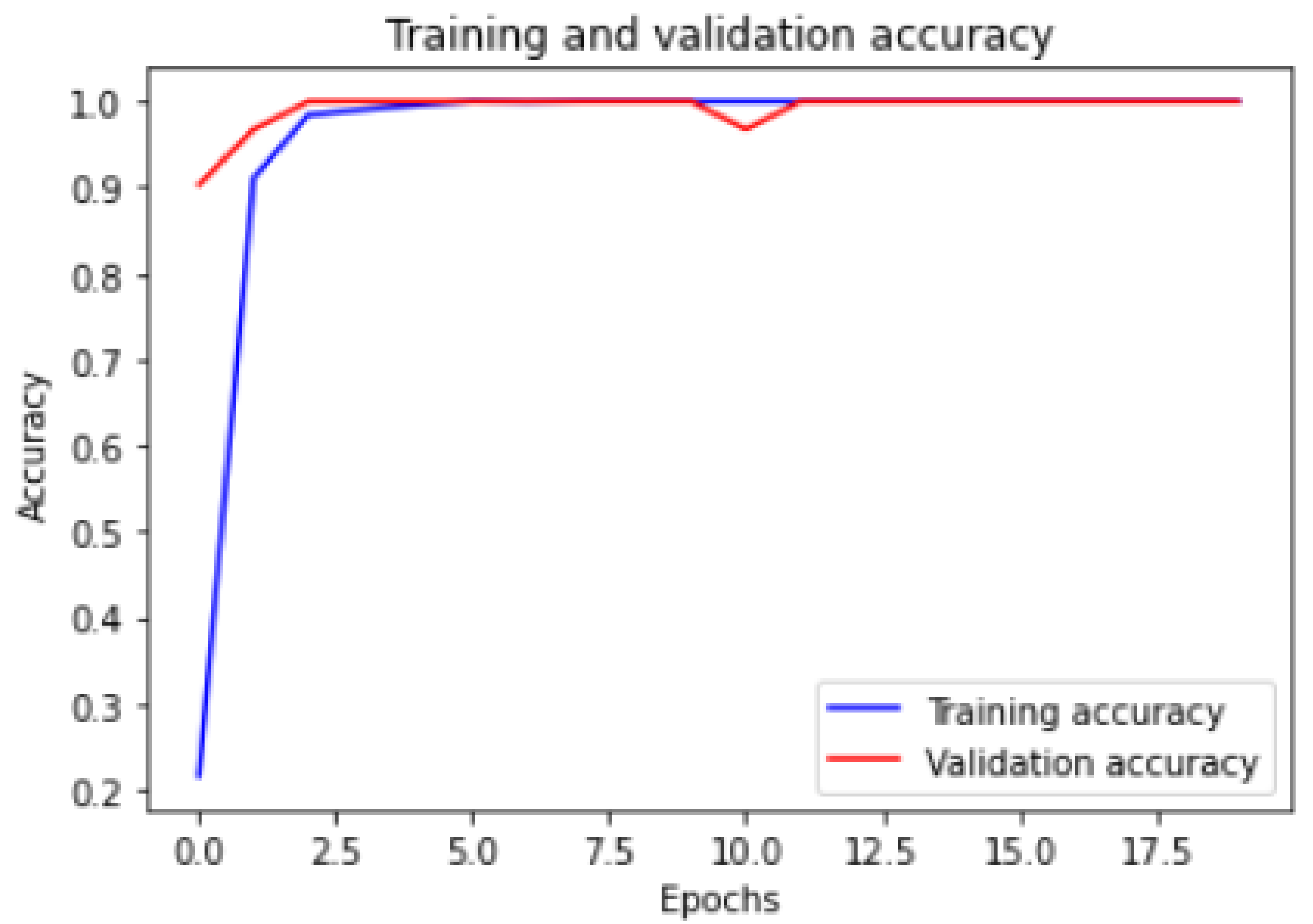
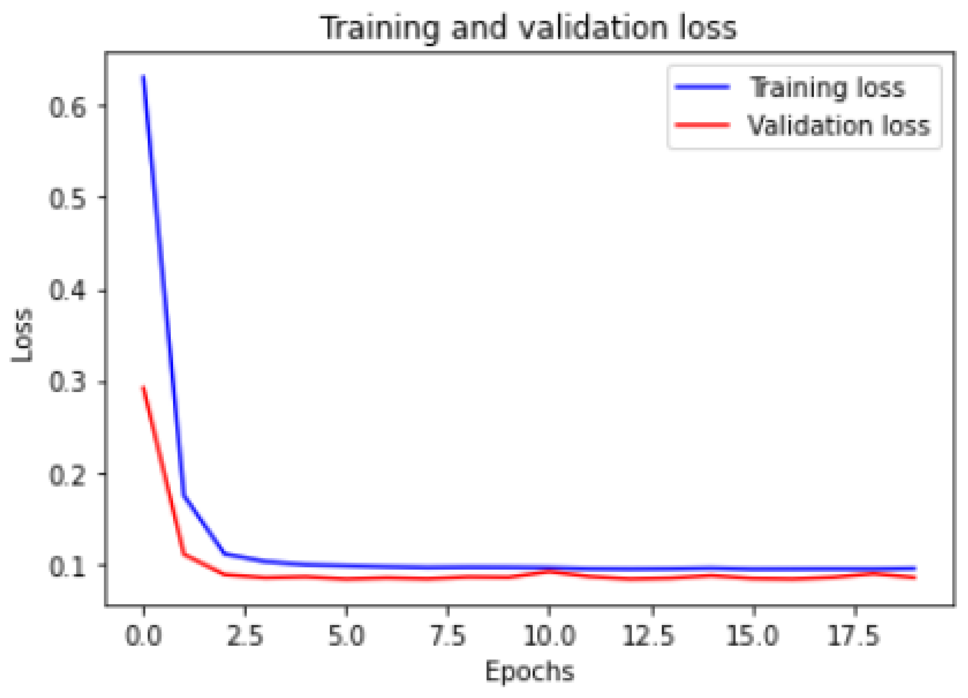
The hyper-parameters have been customized in the network based on the experiments. We have considered the relationship between the loss function and learning rate, optimizer type, calculating stride, dropout values, and the number of epochs. The learning rate controls how quickly the model is adapted to the problem. Smaller learning rates require more epochs given the smaller changes made to the weights each update, whereas larger learning rates result in rapid changes and require fewer training epochs. From
Table 7, we can observe that the hyper-parameters are 20 epochs, 4 BS, the Adam optimizer with (
), and 0.001 for
regularization. This achieved
for ACC,
for DSC,
for AUC,
for precision and recall curve.
Figure 6 and
Figure 7 show the training and validation ACC and loss.
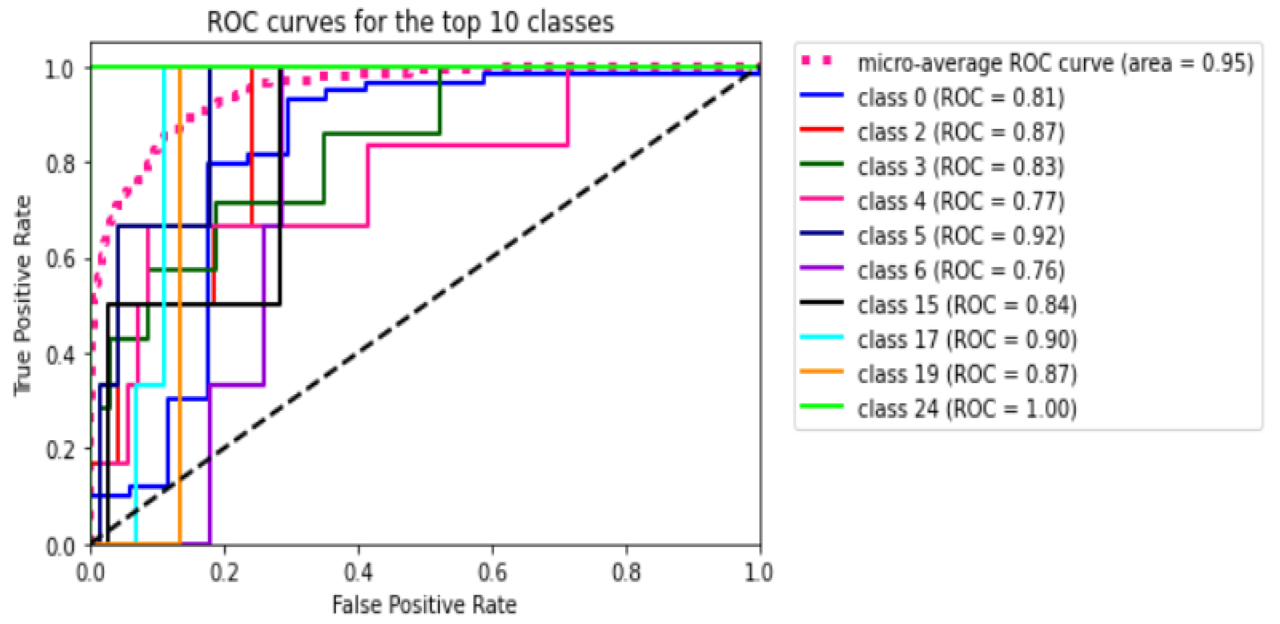
Figure 8 shows the ROC curve for all the 45 classes of the utilized dataset. The figure shows that the micro average ROC curve area for all 45 classes or ODs is
.
Figure 9 shows the precision and recall (PR) curve for all 45 classes of the utilized dataset. The figure shows that the micro average PR curve area for all 45 classes or ODs is
.
The proposed model outputs the images with a title that informs the physician of the predicted ODs by the system and the actual labels or ground truth (GT) of that image.
Figure 10 shows an example of output predictions and the actual GTs. The image in (a) has TSLN disease, but it is predicted that it has DR, TSLN, and MH ODs. On the other hand, the image in (b) has the DR and LS diseases simultaneously, but it is predicted to have TSLN, DR, and MH ODs.
Now, we demonstrate the comparison between the proposed ML-CNN model and the other state-of-the-art models, such as MobileNetV2, DenseNet201, SeResNext50, Xception, InceptionV3, and InceptionresNetv2, through the five performance metrics defined above.
Table 8 shows the resulting averages of ACC, SEN, PREC, DSC, Loss, and AUC for MobileNetV2, DenseNet201, SeResNext50, Xception, InceptionV3, InceptionresNetv2, and the proposed ML-CNN by using dataset split and 10-fold cross-validation techniques. We can observe that the proposed system with a 10-fold cross-validation technique is the best in SEN, PREC, and AUC.
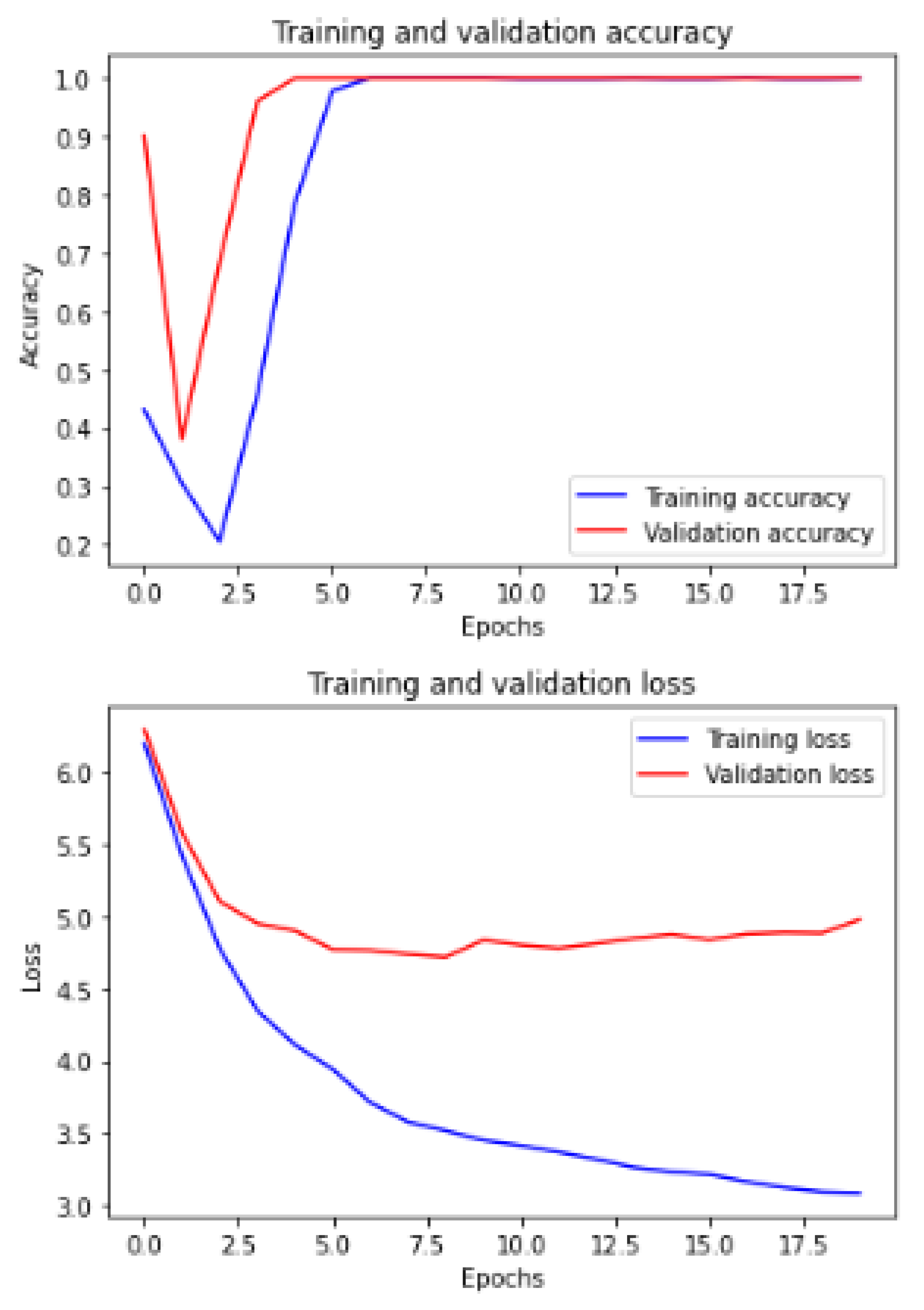
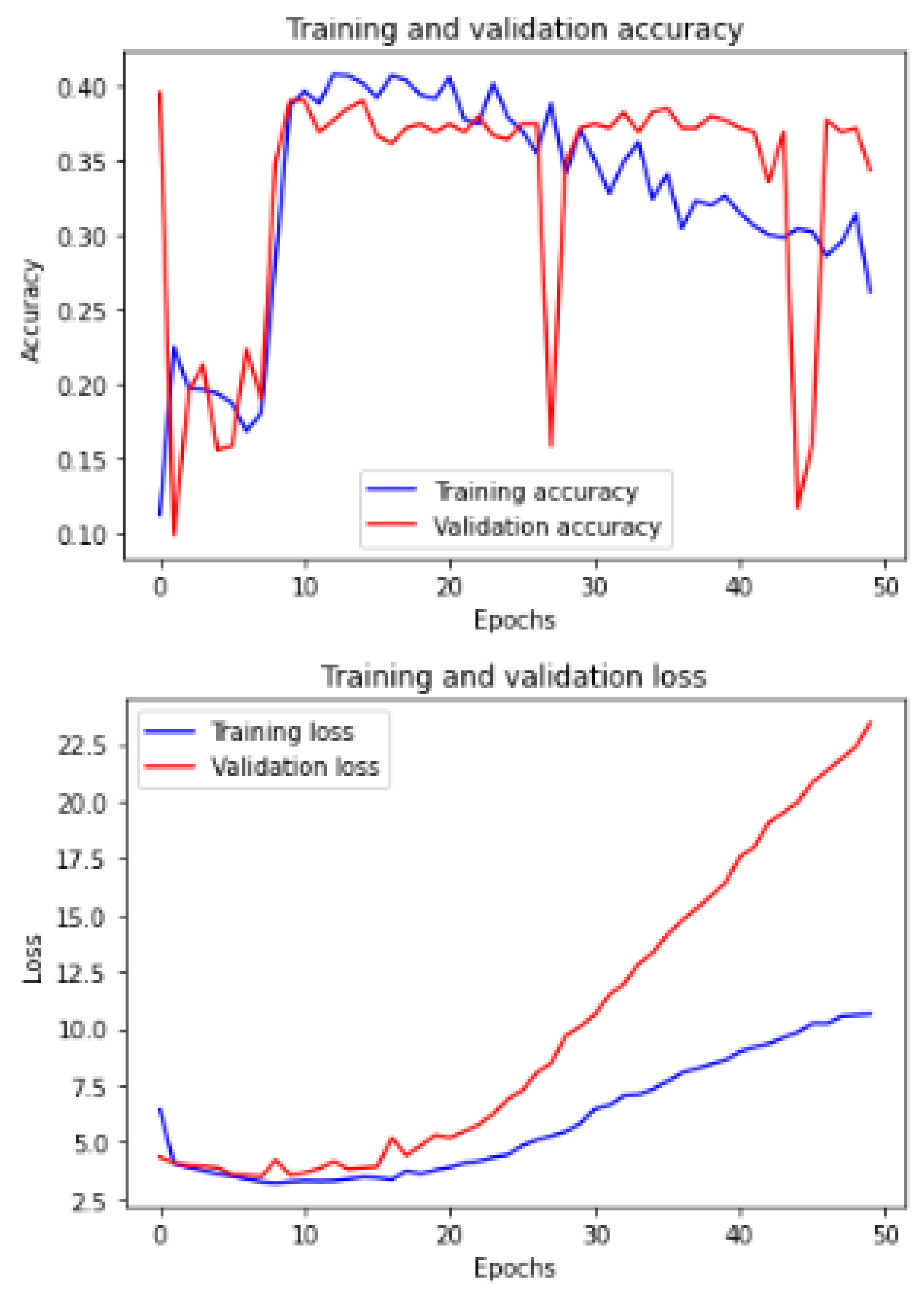
Figure 11 shows the training and validation of ACC and loss of utilizing the InceptionV3 model on the same utilized dataset in our ML-CNN model.
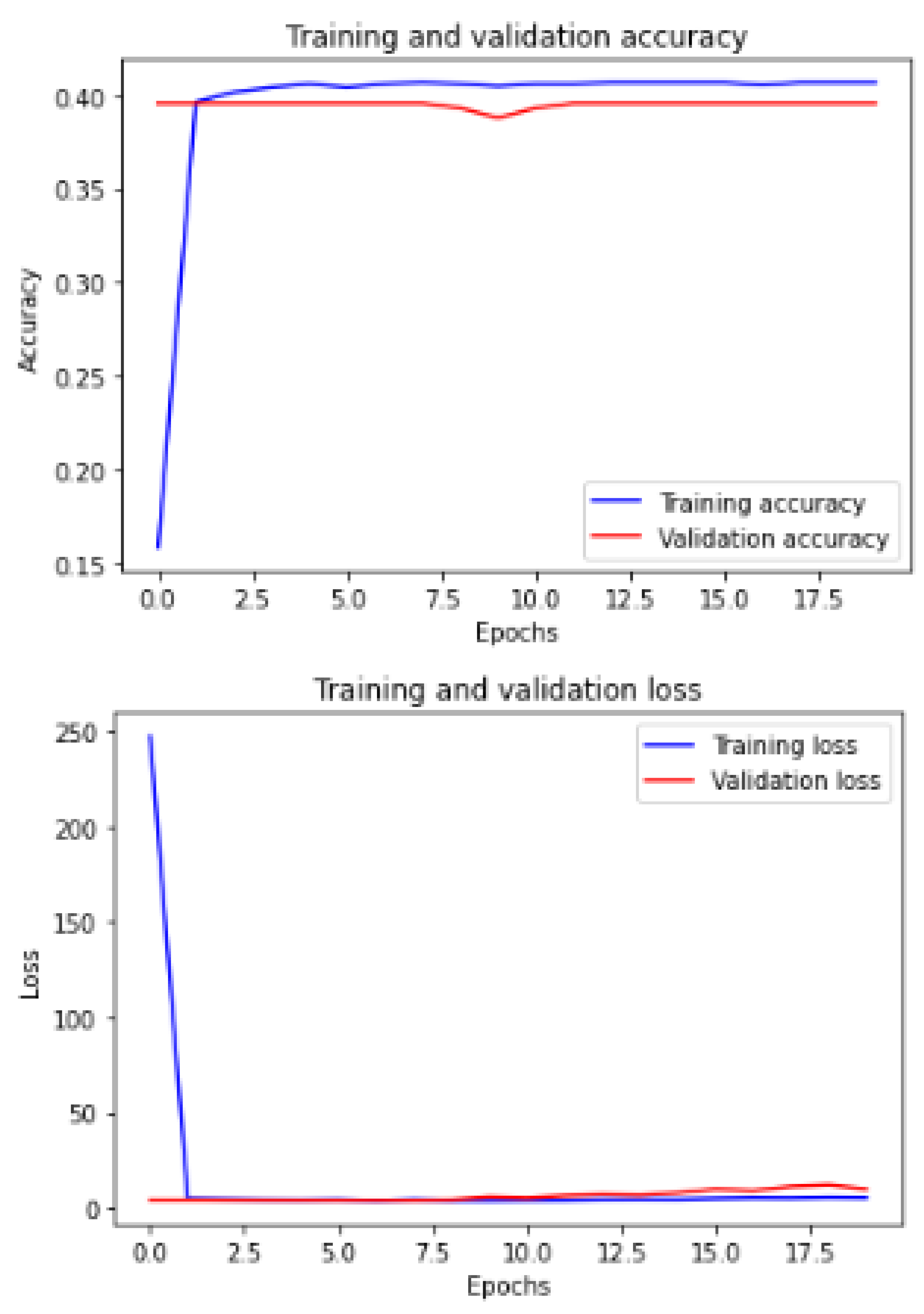
Figure 12 shows the training and validation of ACC and loss of utilizing the mobileNetV2 model on the same utilized dataset in our ML-CNN model.
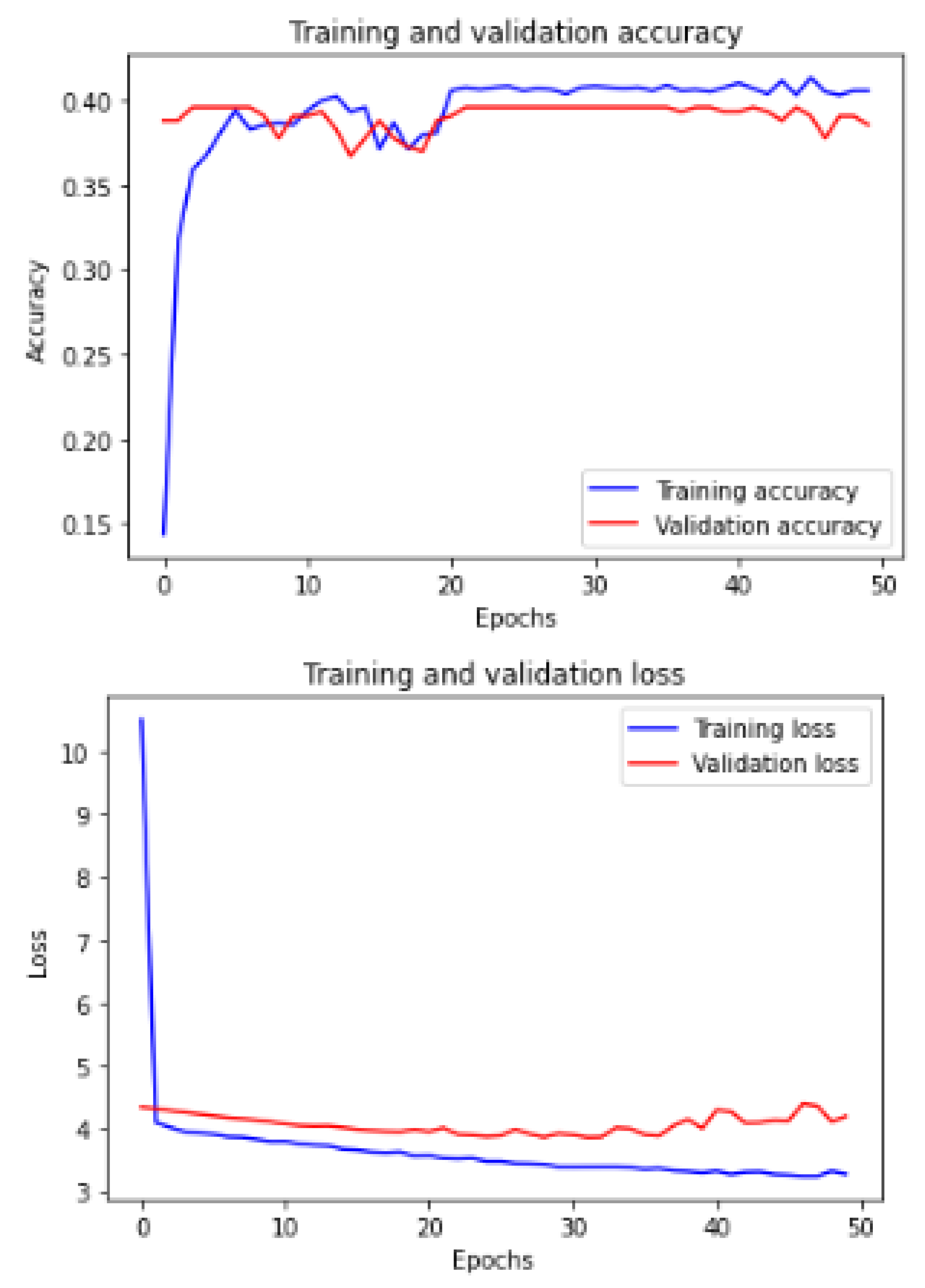
Figure 13 shows the training and validation of ACC and loss of utilizing the DenseNet201 model on the same utilized dataset in our ML-CNN model.
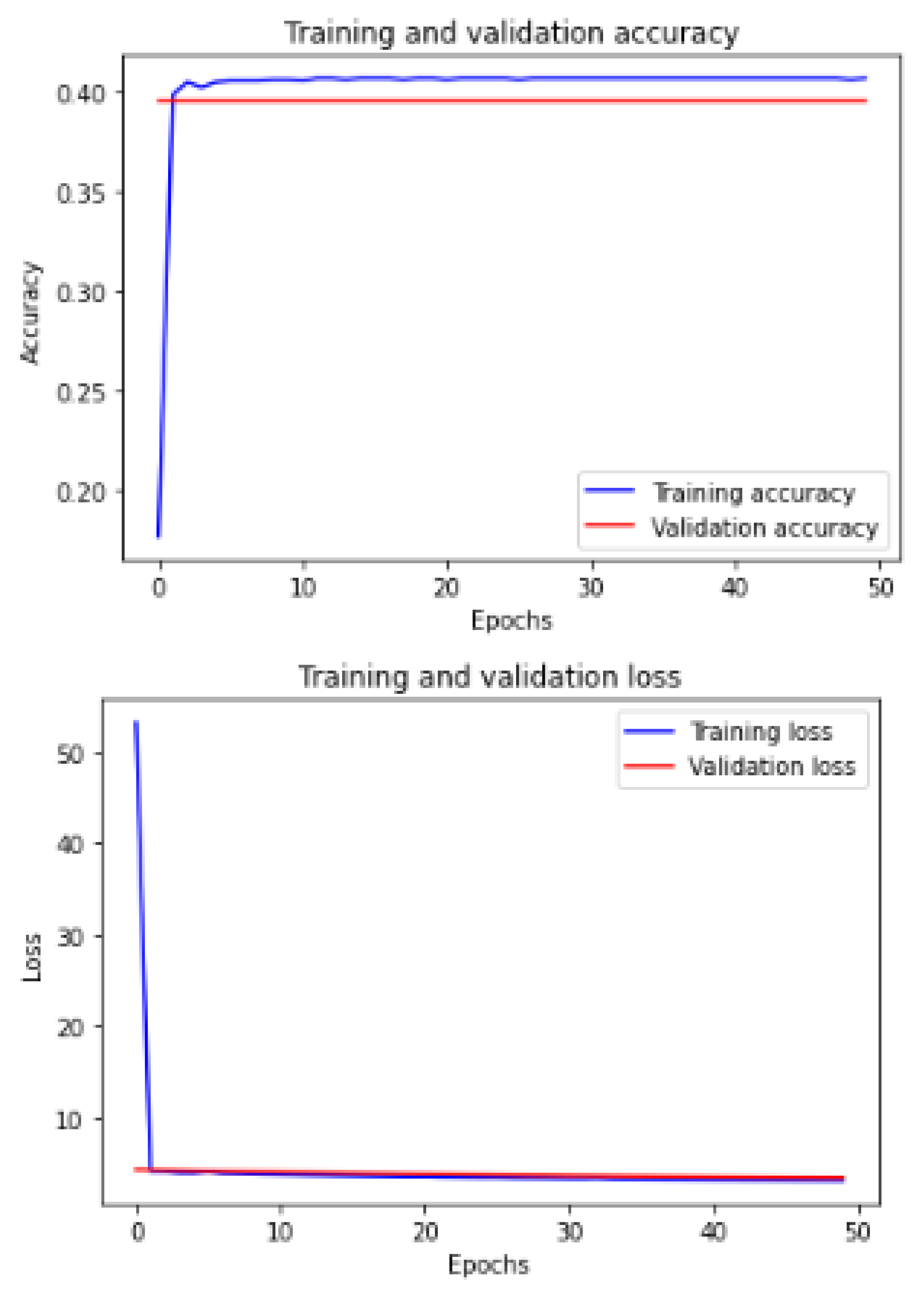
Figure 14 shows the training and validation of ACC and loss of utilizing the seResNext model on the same utilized dataset in our ML-CNN model.
Figure 15 shows the training and validation of ACC and loss of utilizing the Xception model on the same utilized dataset in our ML-CNN model.
Figure 16 shows the training and validation of ACC and loss of utilizing the InceptionResNetV2 model on the same utilized dataset in the ML-CNN model.
4.2.2. K-Fold Cross-Validation
We also evaluated the proposed CAD system using 2-fold cross-validation (CV), 5-fold CV, and 10-fold CV.
Table 9 shows the resulting averages of ACC, SEN, PREC, DSC, Loss, and AUC after applying 2-, 5-, and 10-fold CV. We can observe that the 10-fold CV achieves better results than the others, especially in SEN, PREC, and AUC. The values are
,
, and
, respectively.
Table 10 presents in detail the AUC values for each class or ODs in the 2-, 5-, and 10-fold CV. We notice that all the k-folds CVs could not predict eight classes: TV, CWS, ODPM, HR, TD, VH, VS, and PLQ. On the contrary, DR, AMD, MH, DN, MYA, BRVO, TSLN, CSR, ODC, CRVO, LS, AH, ODP, ODE, and AION can be detected in all folds. The others may be detected in one or two folds.
5. Discussion
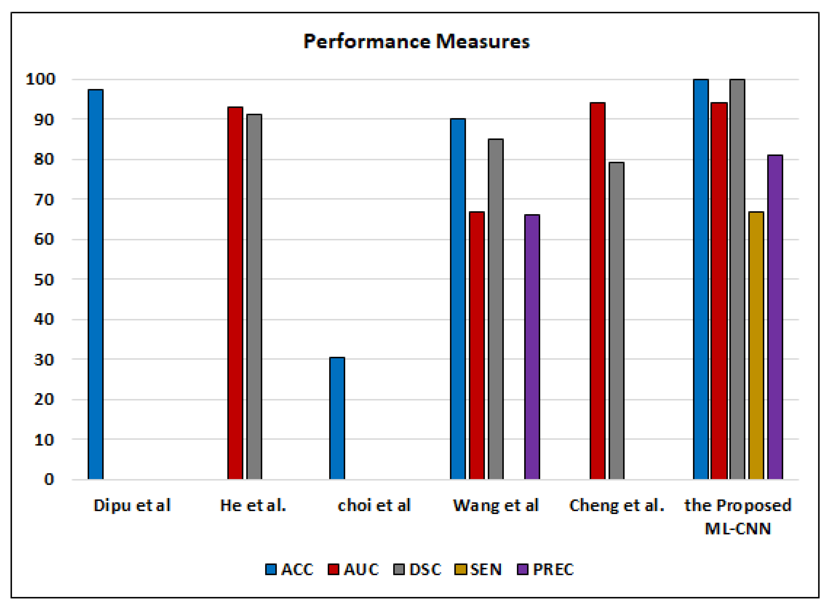
This section provides detailed analytical comparisons between the proposed ML-CNN system and the other studies reported in the literature for detecting various ODs. In the system proposed by Choi et al. [
41], it was observed that increasing the classes to be predicted in MLC decreases the ACC. They achieved
for ACC of classification of ten classes. However, when they predicted only three classes, the ACC increased to
. Wang et al. [
9] achieved
for ACC to make MLC of only eight classes from the ODIR2019 dataset by using the EfficientNet model, while Dipu et al. [
40] achieved
for ACC in 2021. We achieved
,
,
,
, and
for ACC, DSC, AUC, PREC, and SEN, respectively. Apart from PREC and SEN, our system outperforms the system proposed by Wang et al. [
9]. In the proposed ML-CNN, the AUC is higher than what is achieved by He et al. [
8] by
. On the other hand, the proposed ML-CNN system achieved
,
,
,
, and
for ACC, SEN, PREC, DSC, and AUC, respectively, by using 10-fold CV.
Although ML-C suffers from the overlapped classes and is not mutually exclusive, it enables flexible (soft) classification. Each image may include more than one or two ODs simultaneously. If ML-C cannot predict all ODs, the patient is at risk. On the contrary, binary (hard) classification predicts only the presence/absence of the disease. ML-C gives the probability of occurring the ODs in each case. Our results are good enough compared to the other works that employ the ML-C concept to detect various ODs from color fundus images, such as Dipu et al. [
40], He et al. [
8], Wang et al. [
9], Cheng et al. [
39], and Choi et al. [
41], as shown in
Figure 17.
The k-fold CV reduces the overfitting but does not completely eliminate overfitting. Therefore, we will split data manually in the future. The limitations of our system are that it falls into overfitting in some epochs, and SEN/recall could be relatively low. In the case of increasing the epochs, the recall increases, and the ACC decreases.


