GSCINet: Gradual Shrinkage and Cyclic Interaction Network for Salient Object Detection

Abstract

Feature Pyramid Network (FPN) has been widely applied in the task of salient object detection (SOD), which has achieved great performance. However, most existing FPN-based SOD methods still have some limitations, such as insufficient guidance due to gradual dilution of semantic information, excessive computation leading to slow inference speed, and low efficiency of training models. In this paper, we design a novel Gradual Shrinkage and Cyclic Interaction Network (GSCINet) for efficient and accurate SOD, consisting of a Multi-Scale Contextual Attention Module (MSCAM) and an Adjacent Feature Shrinkage and Interaction Module (AFSIM). Specifically, the MSCAM aims at efficiently capturing multi-scale and multi-receptive-field contextual attention information through a series of well-designed convolutions and attention weight matrices of different scales to enhance the performance of initial input features. Subsequently, in AFSIM, we propose a gradual shrinkage structure and introduce a circular interaction mechanism to optimize the compressed features with less calculation cost, thereby enabling fast and accurate inference of salient objects. Extensive experimental results demonstrate the high efficiency and superiority of GSCINet against 17 state-of-the-art (SOTA) saliency detection methods under multiple evaluation metrics.

1. Introduction

Inspired by the human visual perception mechanisms, salient object detection (SOD) is dedicated to detecting and segmenting the most attractive objects or regions from an image or video. With its ability to process data quickly and efficiently, SOD has been widely used as a pre-processing stage in many computer vision tasks, such as image retrieval [1], visual tracking [2], style transfer [3], and image or video compression [4], among several others.

Early SOD methods [5,6,7,8,9] predict saliency maps by using hand-crafted features (e.g., color, texture, contrast). However, these SOD methods have limited capacity for detecting salient objects with complicated contours in cluttered backgrounds due to the under-utilization of high-level semantic information. Recently, the application of convolutional neural networks (CNNs) [10,11] and full convolutional networks (FCNs) [12,13,14,15,16,17,18] has successfully broken these limitations and has been widely used in SOD tasks with its efficient multi-level features extraction ability.

Designing effective model architectures that can capture more powerful feature representations have been a research hotspot in SOD tasks. Additionally, how to utilize complementary information (i.e., high-level semantic information and low-level spatial detail information) from different level features is also a key issue for accurate SOD. One typical architecture used to generate feature representations is the feature pyramid network (FPN) structure [19], which mainly contains an encoder of a bottom-up pathway, a decoder of a top-down pathway, and some side connections. Various SOD methods [12,14,16,20,21,22,23] have been proposed based on the FPN structure and have accomplished great performance. However, when the semantic information of the high-level features guides the low-level features, this semantic information is diluted as the number of network layers increases, and thus it cannot effectively locate salient objects (as illustrated in the last three columns of Figure 1). In addition, the integration of large resolution features will cause high computational load, resulting in slow inference speed and difficulty in model training.

In this paper, we rethink the feature pyramid network (FPN) structure [19] and propose a Gradual Shrinkage and Cyclic Interaction Network (named as GSCINet) for accurate and efficient SOD. The proposed GSCINet method consists of two components, i.e., a Multi-Scale Contextual Attention Module (MSCAM) and an Adjacent Feature Shrinkage and Interaction Module (AFSIM). Unlike classical FPN structure [19], the GSCINet method aims to reduce the computational load and increase the flow of diverse information by progressively aggregating and shrinking adjacent features and a cyclic interaction strategy. More specifically, we first used the MSCAM to simultaneously capture local and global contextual attention information by utilizing light-weight convolutions and channel-attention matrices of different scales, which can help learn more discriminative features effectively. Subsequently, the AFSIM was adopted to gradually aggregate adjacent features and iteratively interact with complementary information at different level features in a cyclic structure to generate high-quality feature representations. Finally, we trained the whole GSCINet network in an end-to-end manner and accomplished superior prediction results compared with 17 state-of-the-art (SOTA) SOD methods on five public benchmark datasets.

In summary, our main contributions are summarized as follows:

(1) We propose a Multi-Scale Contextual Attention Module (MSCAM), which can efficiently extract abundant contextual attention features with different receptive fields to strengthen the performance of each initial input feature.

(2) We constructed an Adjacent Feature Shrinkage and Interaction Module (AFSIM) to reconstruct multi-level features, which is capable of reducing computational cost and interacting with complementary information to generate high-quality feature representations.

(3) Extensive experimental results convincingly demonstrate the significant superiority of the GSCINet method over 17 state-of-the-art SOD methods under different evaluation metrics.

2. Related Work

2.1. Traditional-Based SOD Methods

Over the past two decades, many SOD methods have been proposed to detect and segment salient objects in real-world scenes [6,7,12,13,24,25,26]. Early SOD methods are also called traditional SOD methods, which are mainly based on hand-crafted features (e.g., color [27], contrast [7], and intensity [24]) and some heuristic priors (e.g., spatial distribution prior [5], center prior [6], and background prior [9]) to predict saliency maps, and more details can be found in [28].

Due to the inability to fully exploit high-level semantic features for understanding image contents, these methods [5,6,7,9,24,27] have significant challenges in generating low-quality saliency maps in the face of complex and cluttered scenes. Recently, with the rise of deep learning, fully convolutional networks (FCNs)-based SOD methods [13,15,20,25,29,30], thanks to their ability to efficiently capture and exploit multi-level features, have successfully broken these limitations and greatly improved the accuracy of saliency maps.

2.2. FCNs-Based SOD Methods

Inspired by the great success of FCNs in the semantic segmentation [31], FCNs-based SOD methods can directly predict saliency maps instead of classification scores of image blocks, which can not only greatly improve the computational efficiency, but also extract more significant feature information. Most of the structures of these methods [12,13,14,15,20,21,23,26] are based on a feature pyramid network (FPN) [19], as depicted in Figure 2a. For example, Zhang et al. [12] utilized the reformulated dropout after several convolutional layers to learn uncertain convolutional features for the SOD task. Next, Wang et al. [14] designed a localization-to-refinement network, where the former can better localize salient objects and the latter helps refine saliency maps. Zhang et al. [13] devised a bi-directional structure based on FPN to pass messages between multi-level features, where a gate function was exploited to control the message passing rate. To compensate for the gradual dilution of top-down semantic information in FPN architecture, Liu et al. [20] developed a pyramid pooling module (PPM). Feng et al. [21] introduced a residual learning strategy in the FPN structure to gradually align the prediction for accurate SOD. Li et al. [26] proposed a stacked U-shape network with channel-wise attention to enhance the discriminant ability of feature representations for saliency detection. Mei et al. [23] embedded a dense context exploration (DCE) module into the FPN structure to enhance the ability of the network to learn salient features.

Although these methods have achieved great performance, they may infer salient objects slowly and generate inaccurate saliency maps due to the limitations of the FPN structure. To alleviate this problem, we designed a novel GSCINet network structure (schematically shown in Figure 2b) that adequately captures the explicit and implicit information and iteratively aggregates complementary information to generate high-quality feature representations by adopting a shrink interaction strategy, thus achieving efficient and accurate saliency detection.

3. The Proposed GSCINet Methods

In this section, we first present the overall architecture of the proposed GSCINet method in Section 3.1. We then introduce two principal components (i.e., MSCAM and AFSIM) in Section 3.2 and Section 3.3 to elaborate the GSCINet method. Finally, in Section 3.4, we describe the loss function of our training network.

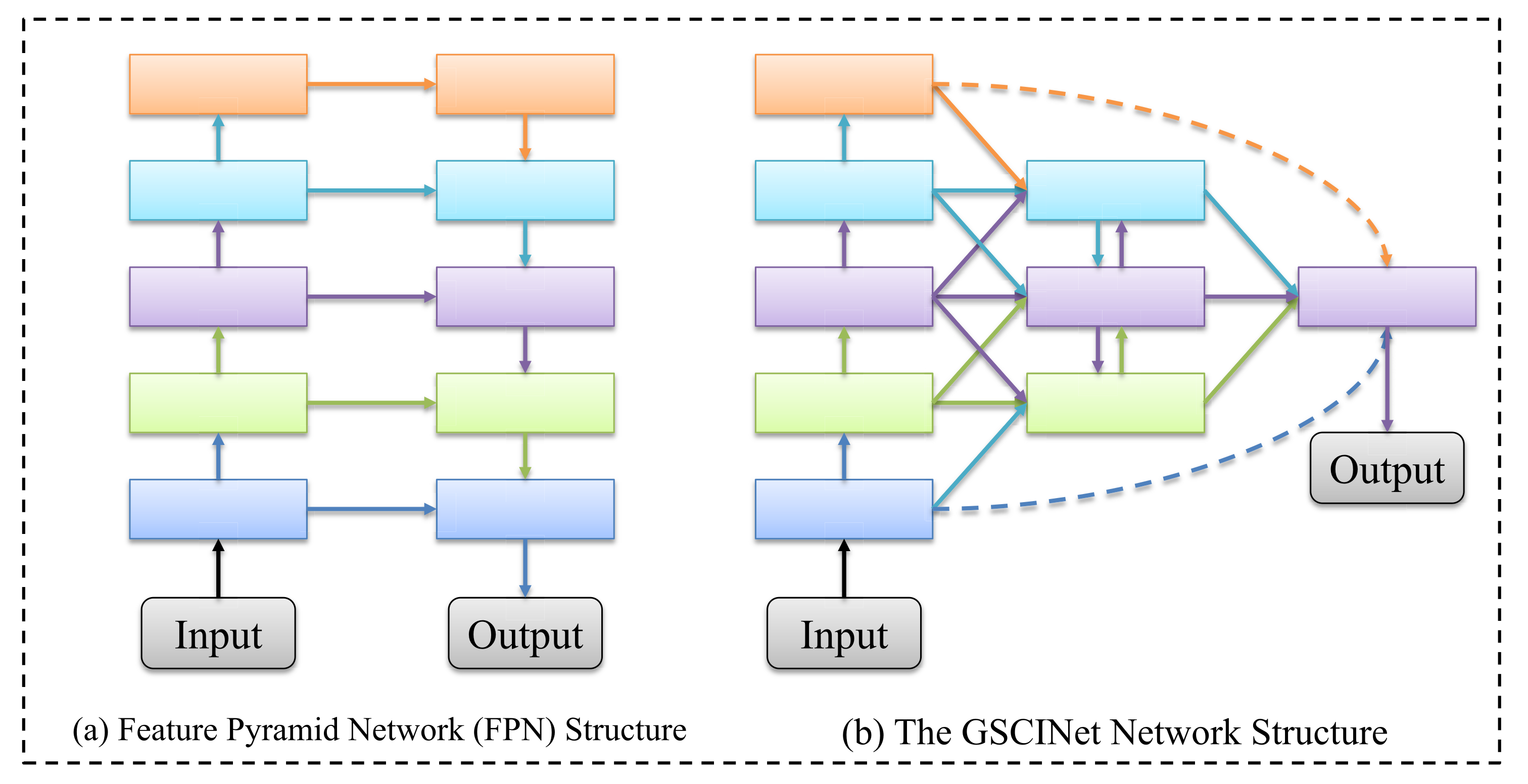
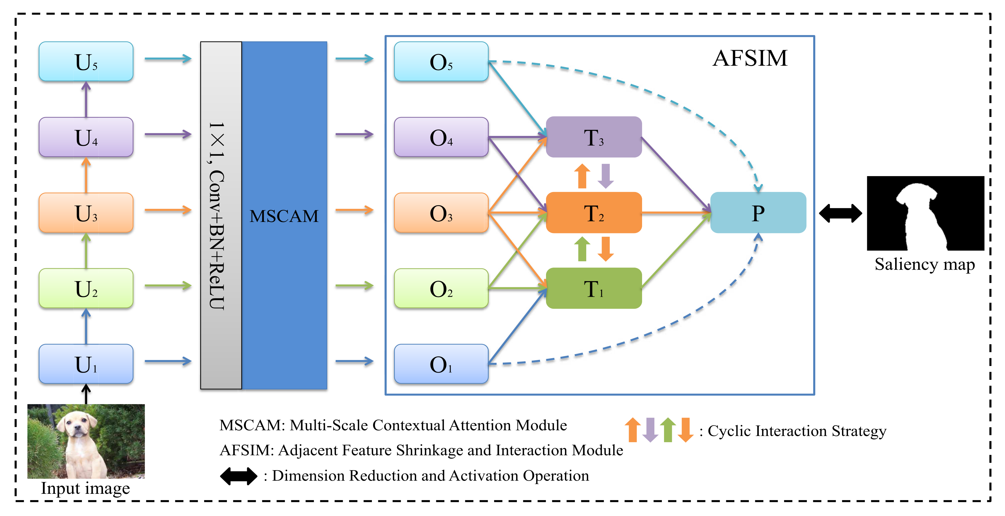
3.1. Overall Architecture

Figure 3 depicts the complete architecture of the proposed GSCINet method. It mainly contains two novel modules, i.e., a Multi-Scale Contextual Attention Module (MSCAM) and an Adjacent Feature Shrinkage and Interaction Module (AFSIM). The MSCAM first efficiently captures local and global contextual attention information to enhance the performance of initial multi-level features at each layer by utilizing multiple dilated depth-wise separable convolutions with different receptive fields and attention weights matrices of different scales. In this way, the initial features are optimized to have richer saliency information. After MSCAM, the AFSIM aggregates all optimized features through an adjacent combination manner to progressively shrink the quantity and resolution of multi-level features and then adaptively interacts with complementary information at each layer feature by utilizing a recurrent strategy. Finally, the interacted features are aggregated again to generate high-quality feature representations, and then we applied a convolution layer with a 1 × 1 kernel and a sigmoid function on the feature to predict the final saliency map.

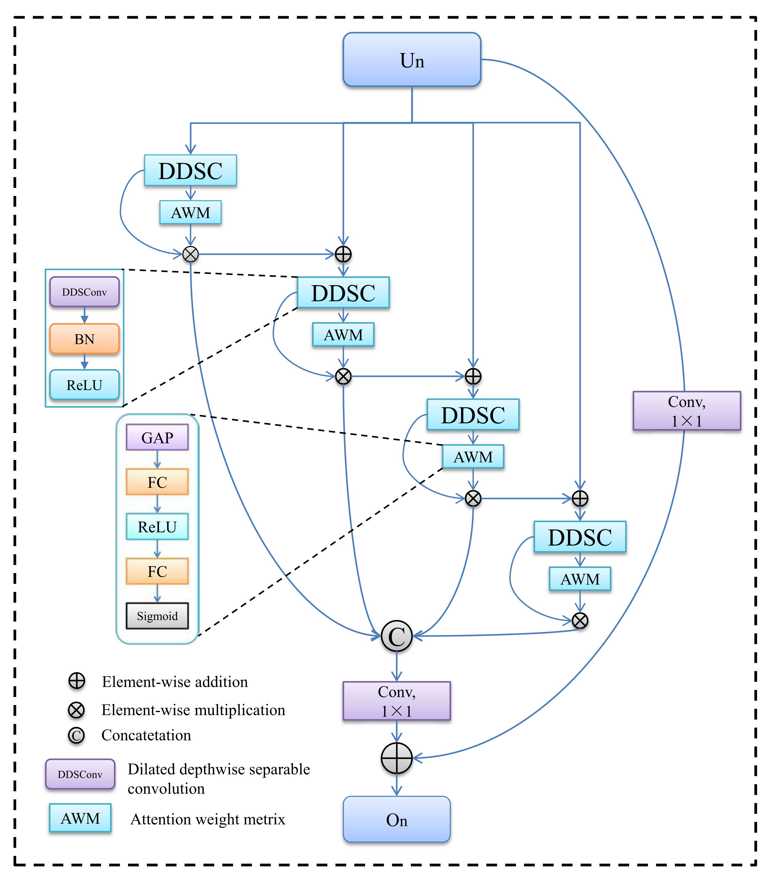
3.2. Multi-Scale Contextual Attention Module (MSCAM)

For the SOD task, it is necessary to extract abundant contextual information for efficiently locating and segmenting salient objects. Some existing SOD methods [13,26,29,30,32,33] use different convolutions to capture contextual information and have achieved significant performance. However, not all contextual information is relevant to the salient objects in the feature channels, and on the contrary, some noise information may interfere with the prediction of salient objects. In addition, the superposition of a large number of convolutions will greatly increase the parameters and computation. At this point, we design the MSCAM that captures different scale contextual attention information with fewer parameters to increase the effectiveness of positive contextual information. In this module, the representational power of all initial multi-level features is enhanced, benefiting from the integrated multi-scale contextual attention features. Figure 4 shows the architecture of the proposed MSCAM.

Specifically, we took the ResNet-50 [34] as the backbone network to extract initial multi-level features $U=\{U_1,U_2,U_3,U_4,U_5\}$ from the first pooling layer and the following four convolutional blocks of the backbone. We used a convolution layer with a 1 × 1 kernel, a Batch Normalization (BN) and a ReLU activation function on each level feature for dimension reduction, resulting in each feature with a channel number of 128. Unlike previous methods [13,14,23,25,26,32], the MSCAM adopts multiple dilated depth-wise separable convolutions with different dilation rates (i.e., 0, 2, 4, 6) to capture multi-receptive-field contextual information with fewer parameters and computation. It should be noted that contextual information at different scales is correlated due to the introduction of side connections. As depicted in Figure 4, in different branches, dilated depth-wise separable convolutions with different dilation rates are applied to each input initial feature. Therefore, we calculated multi-scale contextual information ($M_i$) of $U_n$$(n=1,2,3,4,5)$ as follows:

$$\begin{array}{c}\hfill \left\{\begin{array}{c}{M}_i={\mathfrak{A}}_i(\delta \left(U_n\right)),i=1\hfill \\ M_i={\mathfrak{A}}_i(\delta \left(U_n\right)+M_{i-1}),i=2,3,4\hfill \end{array}\right.\end{array}$$

(1)

where ${\mathfrak{A}}_i$ denotes the dilated depth-wise separable convolution at branch i and $\delta$ represents a dimension reduction that contains a convolution layer with 1 × 1 × 128 kernel, a Batch Normalization (BN), and a ReLU activation function.

Considering the inequality of information at different feature channels, we attempted to leverage the captured multi-scale contextual information $M_i$ to learn diverse attention matrices for the purpose of selecting more useful information. To this end, the MSCAM uses a series of dimensionality reduction and activation operations to generate the channel-attention weight matrix $\mathcal{A}$, i.e.,

$$\begin{array}{c}\hfill \mathcal{A}=\sigma |F_2(\tau \left(F_1(\lambda \left(M_i\right))\right))|,\end{array}$$

(2)

where $\sigma$ denotes the sigmoid function, $F_1$ and $F_2$ are two fully connected (FC) layers, $\tau$ represents the ReLU function, $\lambda$ is global average pooling operation, and $M_i$ presents multi-scale contextual information. As a result, we can realize the selection of important object information from different feature channels based on Equation (2). With the attention weight $\mathcal{A}$, we effectively strengthen the performance of each multi-scale contextual feature. The mathematical formula is defined as:

$$\begin{array}{c}\hfill \widehat{M_i}=M_i\otimes {\mathcal{A}}_i,i=1,2,3,4\end{array}$$

(3)

where ${\mathcal{A}}_i$ is the ith element in the $\mathcal{A}$ and ⊗ denotes element-wise multiplication. Contextual attention information at different scales is then aggregated by a single concatenation, and residual connections are introduced to generate features $O=\{O_1,O_2,O_3,O_4,O_5\}$ with abundant saliency information, i.e.,

$$\begin{array}{c}\hfill O_n=\gamma \left(Cat(\widehat{M_1},\widehat{M_2},\widehat{M_3},\widehat{M_4})\right)+\gamma \left(U_n\right),n=1,2,3,4,5\end{array}$$

(4)

where $\gamma$ represents the dimension reduction and $Cat$ and + denote the concatenation and element-wise addition, respectively.

3.3. Adjacent Feature Shrinkage and Interaction Module (AFSIM)

Intuitively, the different level features are complementary [13,21,22,25,35], i.e., high-level features containing rich semantic information are helpful for locating the salient objects, while low-level features can provide the spatial detail information to complement the boundaries of the salient objects. The classical FPN structure [19] uses side connections to transfer the information between features at the same scale, which interact with information of the different scale features via a top-down pathway. Based on the above observation, the top-level features are progressively up-sampled and then fused with the corresponding features in the top-down pathway to increase the semantic information of the bottom-level features. However, semantic information is continuously diluted in the process of continuous aggregation, resulting in not much semantic information actually reaching the bottom-level features. In addition, due to the ever-expanding resolution of downward aggregation features, this kind of structural reasoning speed is slow and time-consuming to train. For that, we designed the AFSIM to progressively shrink and circularly restructure multi-level features for fast and accurate SOD tasks.

Figure 3 gives the structure of the proposed AFSIM. Specifically, the AFSIM consists of three steps, i.e., shrinkage, interaction, and aggregation. Firstly, we adopted a combination of adjacent features to reduce the number of multi-level features, thereby realizing the gradual reduction of five sub-layer features into three sub-layer features $T=\{T_1,T_2,T_3\}$, which can be represented as:

$$\begin{array}{c}\hfill T_i=O_{i+2}+O_{i+1}+O_i,i=1,2,3\end{array}$$

(5)

where + denotes element-wise addition and O presents multi-level features from the MSCAM. Note that we used the element-wise addition instead of concatenation, which is mainly based on the fact that the latter will greatly increase the number of feature channels, resulting in high computational cost. Secondly, considering the complementarity of different level features, different from [15,22,25,33,35] employing a single top-down interaction manner, we interacted with multi-level features T via a circular interaction strategy, i.e.,

$$\begin{array}{c}\hfill \left\{\begin{array}{c}{T}_2=T_2+T_3\hfill \\ \widetilde{T_1}=T_1+T_2\hfill \\ \widetilde{T_2}=\widetilde{T_1}+T_2\hfill \\ \widetilde{T_3}=\widetilde{T_2}+T_3\hfill \end{array}\right.,\end{array}$$

(6)

where $\widetilde{T_n}$ denotes the interacted multi-level feature at the nth level. Finally, to further increase the semantic information and spatial detail information, we again aggregated the interacted multi-level feature $\widetilde{T_n}$ with the top-level feature $O_5$ and the bottom-level feature $O_1$ to generate a high-quality feature representation P. The entire process was formulated as follows:

$$\begin{array}{c}\hfill P=\widetilde{T_1}+\widetilde{T_2}+\widetilde{T_3}+O_5+O_1.\end{array}$$

(7)

Through the collaboration of MSCAM and AFSIM, the performance of each initial multi-level $U_n$ is remarkably improved. Moreover, the number of the optimized multi-level features are shrunk to reduce the calculation and improve reasoning efficiency. Additionally, the high-level semantic information and the low-level spatial structure details are adaptively interacted to gradually reconstruct and strengthen the features. Overall, this enables the proposed GSCINet method to efficiently and accurately predict salient objects with complicated structures in cluttered real-world scenes.

3.4. Loss Function

Given the aggregated features, we appended a 1 × 1 convolution layer, along with a sigmoid activation function to produce the initial saliency maps. To obtain complete saliency maps with sharp boundaries, we trained the GSCINet network with a hybrid loss defined as:

$$\begin{array}{c}\hfill {\mathfrak{I}}_{Hybird}={\mathfrak{I}}_{BCE}+{\mathfrak{I}}_{IoU},\end{array}$$

(8)

where ${\mathfrak{I}}_{BCE}$ and ${\mathfrak{I}}_{IoU}$ denote binary cross-entropy(BCE) loss function [36] and IoU loss function [37].

The BCE loss function [36] is most widely used in segmentation and binary classification, which is calculated as follows:

$$\begin{array}{c}\hfill {\mathfrak{I}}_{BCE}=-\sum _{(m,n)}[Y(m,n)log\left(X(m,n)\right)+(1-Y(m,n))log(1-X(m,n))],\end{array}$$

(9)

where X and Y present the predicted salient object and ground truth, respectively. Both $X(m,n)$∈ [0, 1] and $Y(m,n)$∈ {0, 1} are the probability of the salient objects at the position $(m,n)$. However, the BCE loss function that only focuses on the loss of each individual pixel always ignores the loss of part of the complete structure in the images, and it is not conducive to supervising the generation of saliency maps with better quality. Hence, we introduced the IoU loss function [37] to concentrate on more complete saliency regions, formulated as:

$$\begin{array}{c}\hfill {\mathfrak{I}}_{IoU}=1-\frac{{\displaystyle \sum _{(m,n)}}[X(m,n) \times Y(m,n)]}{{\displaystyle \sum _{(m,n)}}[Y(m,n) + X(m,n) - Y(m,n) \times X(m,n)]},\end{array}$$

(10)

We adopted the Adam optimizer to train the proposed GSCINet method, and it directly generated the final saliency maps without any post-processing.

4. Experiment

4.1. Datasets

We comprehensively evaluated the proposed GSCINet method on five public benchmark datasets, including ECSSD [38], PASCAL-S [39], HKU-IS [40], DUT-OMRON [41], and DUTS-TE [42]. The ECSSD [38] and PASCAL-S [39] datasets consist of relatively small of 1000 and 850 images, respectively. Some images in these two datasets contain cluttered backgrounds, which are very challenging. The HKU-IS [40] dataset consists of 4447 images with multiple salient objects. The DUT-OMRON [41] dataset comprises 5168 images with complicated structures and different types. The DUTS-TE [42] dataset, derived from the DUTS dataset, has 5019 images usually used for testing.

4.2. Experimental Details

We implemented the GSCINet method with the PyTorch framework on a PC equipped framework NVIDIA 2080Ti GPU. The pre-trained ResNet-50 [34] network is adopted to capture different level features. In the training process, each input image is resized at a resolution of 320 × 320, and data augmentation is carried out by using random horizontal flipping and rotation. We used the Adam optimizer with the momentum of 0.9 and the weight decay of 5 × 10⁻⁴ for loss optimization. Additionally, the initial learning rate was 5 × 10⁻⁵, and the batch size was set to 12. It took about 10 h for our method to converge for 150 epochs. During testing, the images were resized to 320 × 320 for network inference. There was no post-processing (e.g., fully connected conditional random field (CRF)) to improve the performance of the final predicted saliency maps. The proposed GSCINet method can detect salient objects at a real-time speed of 40 FPS.

4.3. Evaluation Metrics

We used multiple standard evaluation metrics to test the performance of the GSCINet method, including the Precision-Recall ($PR$) curve, F-measure ($F_m$) curve, Mean Absolute Error ($MAE$), Average F-measure ($A{F}_m$), Weight F-measure ($W{F}_m$), and E-measure ($E_m$).

$PR$ curve: The $PR$ curve contains precision and recall scores that are computed by comparing the saliency maps with the ground truths to plot the $PR$ curve with different thresholds in the range of [0, 255].

F-measure ($F_m$) : $F_m$ is computed by the weighted harmonic mean of precision and recall to balance the importance of precision and recall, which is defined as follows:

$$\begin{array}{c}\hfill F_m=\frac{(1 + {\beta }^2) \times Precision \times Recall}{{\beta }^2 \times Precision \times Recall},\end{array}$$

(11)

where ${\beta }^2$ is set to 0.3 to emphasize the precision over recall [43], and we adopted both Average F-measure ($A{F}_m$) and Weight F-measure ($W{F}_m$) for comparison of our GSCINet and other SOD methods.

Mean Absolute Error ($MAE$): $MAE$ measures the pixel-level difference between the saliency maps X and the ground truths Y, which is calculated by:

$$\begin{array}{c}\hfill MAE=\frac{1}{W \times H}\sum _{m=1}^W\sum _{n=1}^H|X(m,n)-Y(m,n)|,\end{array}$$

(12)

where H and W are height and width of the input images, respectively. $X(m,n)$ is the saliency value of the pixel at $(m,n)$.

E-measure ($E_m$) [44]: $E_m$ estimates the similarity between the saliency maps X and the ground truths Y by computing local and global similarities and combining local pixel values with image-level averages. It is defined as:

$$\begin{array}{c}\hfill E_m=\frac{1}{W \times H}\sum _{m=1}^W\sum _{n=1}^H\mathcal{C}\left(t\right),\end{array}$$

(13)

where t is the alignment matrix and $\mathcal{C}\left(t\right)$ denotes the enhanced alignment matrix.

4.4. Comparison With State-of-the-Arts

To demonstrate the proposed GSCINet method, we quantitatively and qualitatively compared it with 17 state-of-the-art SOD methods, including UCF [12], Amulet [25], DGRL [14], RASNet [45], BDMPM [13], PoolNet [20], BASNet [16], TSPOANet [46], AFNet [15], CPD [32], R2Net [21], CAGNet [29], GateNet [22], ITSD [47], DSRNet [30], CANet [33], and SUCA [26]. For a fair comparison, all the comparative saliency maps were directly provided by authors or running the available source codes. In addition, the different evaluation values of all saliency maps were generated by using the same evaluation code.

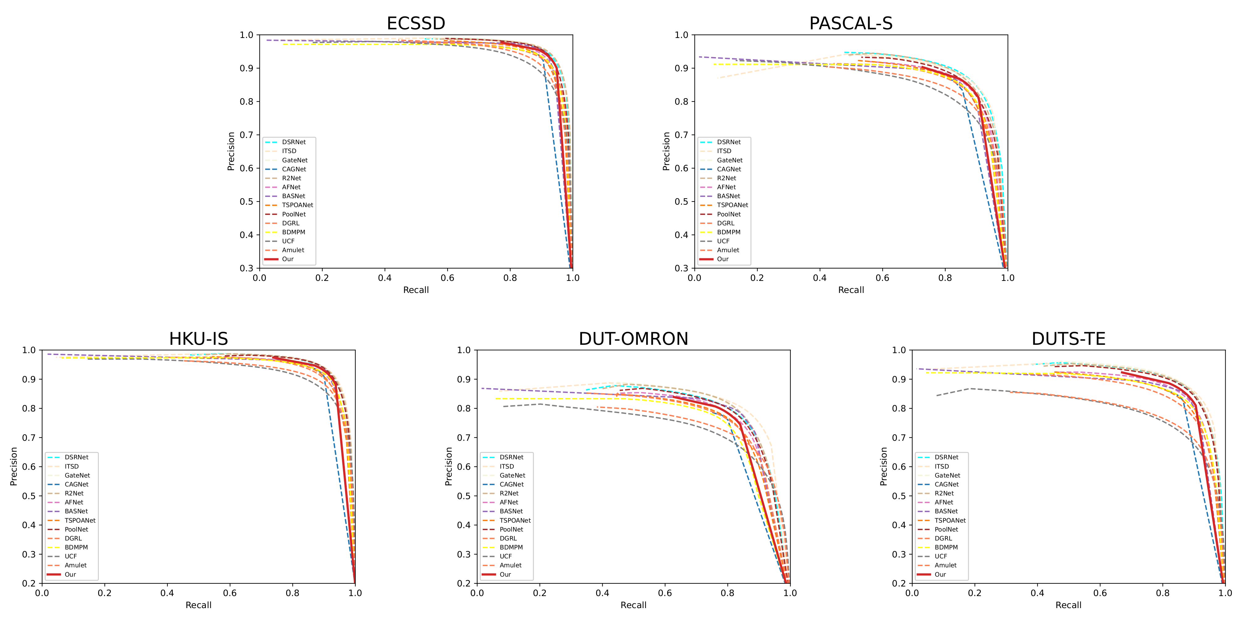
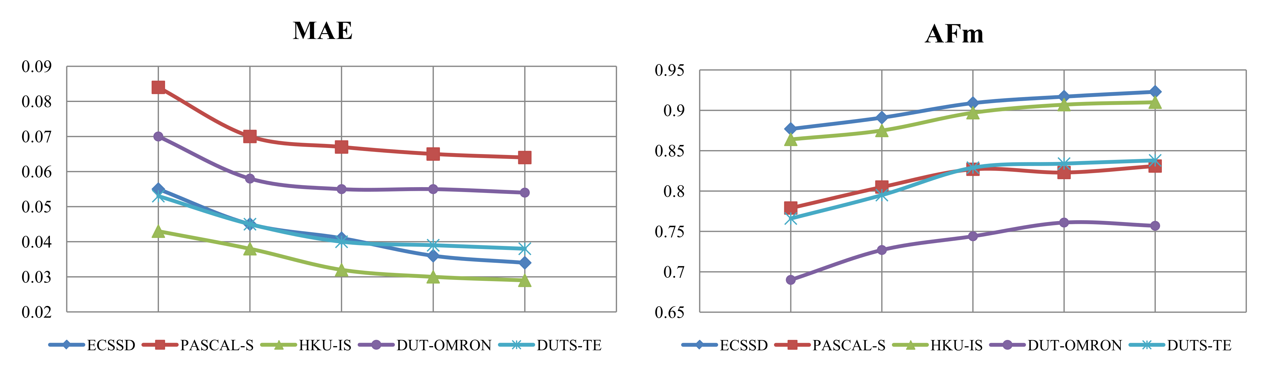
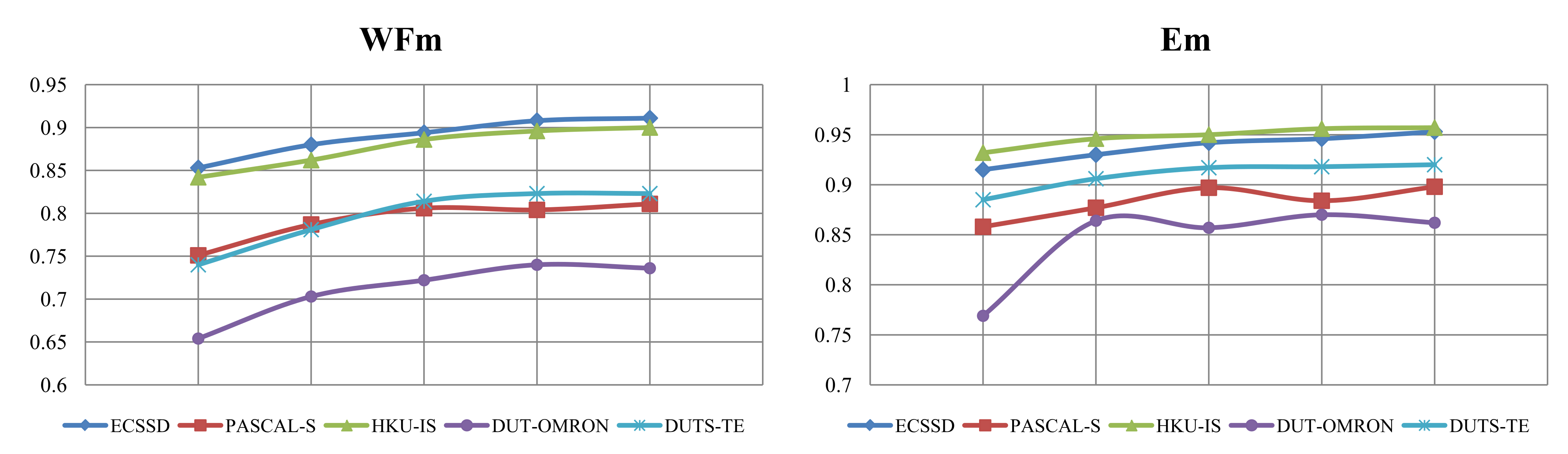
4.4.1. Quantitative Evaluation

Table 1. Quantitative results on five public SOD datasets: the top three results are marked with red, green, and blue. The symbols “↑/↓” indicate that the larger the result, the better, and the smaller the result, the better.

Method	Year, Pub	ECSSD (1000)				PASCAL-S (850)				HKU-IS (4447)				DUT-OMRON (5168)				DUTS-TE (5019)
		$\mathbf{MAE}$↓	${\mathbf{AF}}_{\mathbf{m}}$↑	${\mathbf{WF}}_{\mathbf{m}}$↑	${\mathbf{E}}_{\mathbf{m}}$↑	$\mathbf{MAE}$↓	${\mathbf{AF}}_{\mathbf{m}}$↑	${\mathbf{WF}}_{\mathbf{m}}$↑	${\mathbf{E}}_{\mathbf{m}}$↑	$\mathbf{MAE}$↓	${\mathbf{AF}}_{\mathbf{m}}$↑	${\mathbf{WF}}_{\mathbf{m}}$↑	${\mathbf{E}}_{\mathbf{m}}$↑	$\mathbf{MAE}$↓	${\mathbf{AF}}_{\mathbf{m}}$↑	${\mathbf{WF}}_{\mathbf{m}}$↑	${\mathbf{E}}_{\mathbf{m}}$↑	$\mathbf{MAE}$↓	${\mathbf{AF}}_{\mathbf{m}}$↑	${\mathbf{WF}}_{\mathbf{m}}$↑	${\mathbf{E}}_{\mathbf{m}}$↑
UCF	2017, ICCV	0.069	0.844	0.806	0.896	0.116	0.726	0.689	0.807	0.062	0.823	0.779	0.904	0.120	0.621	0.574	0.768	0.112	0.631	0.596	0.770
Amulet	2017, CVPR	0.059	0.868	0.840	0.912	0.100	0.757	0.728	0.827	0.051	0.841	0.817	0.914	0.098	0.647	0.626	0.784	0.085	0.678	0.658	0.803
DGRL	2018, CVPR	0.046	0.893	0.871	0.935	0.077	0.794	0.772	0.869	0.041	0.875	0.851	0.943	0.066	0.711	0.688	0.847	0.054	0.755	0.748	0.873
BDMPM	2018, CVPR	0.045	0.869	0.871	0.916	0.074	0.758	0.774	0.845	0.039	0.871	0.859	0.938	0.064	0.692	0.681	0.839	0.049	0.746	0.761	0.863
RASNet	2018, ECCV	0.056	0.889	0.857	0.922	0.101	0.777	0.731	0.838	-	-	-	-	0.062	0.713	0.695	0.849	0.059	0.751	0.740	0.864
PoolNet	2019, CVPR	0.039	0.915	0.896	0.945	0.075	0.815	0.793	0.876	0.032	0.900	0.883	0.955	0.056	0.739	0.721	0.864	0.040	0.809	0.807	0.904
BASNet	2019, CVPR	0.037	0.880	0.904	0.921	0.076	0.771	0.793	0.853	0.032	0.896	0.889	0.946	0.057	0.756	0.751	0.869	0.048	0.791	0.803	0.884
AFNet	2019, CVPR	0.042	0.908	0.886	0.941	0.070	0.815	0.792	0.885	0.036	0.888	0.869	0.948	0.057	0.739	0.717	0.860	0.046	0.793	0.785	0.895
CPD	2019, CVPR	0.037	0.917	0.898	0.950	0.071	0.820	0.794	0.887	0.033	0.895	0.879	0.952	0.056	0.747	0.719	0.873	0.043	0.805	0.795	0.904
TSPOANet	2019, ICCV	0.046	0.900	0.876	0.935	0.077	0.804	0.775	0.871	0.038	0.882	0.862	0.902	0.061	0.716	0.697	0.850	0.049	0.776	0.767	0.885
R2Net	2020, TIP	0.038	0.914	0.899	0.946	0.069	0.817	0.793	0.880	0.033	0.896	0.880	0.954	0.054	0.744	0.728	0.866	0.041	0.801	0.804	0.901
CAGNet	2020, PR	0.042	0.914	0.892	0.939	0.076	0.819	0.789	0.882	0.034	0.905	0.885	0.947	0.057	0.744	0.718	0.859	0.045	0.822	0.797	0.904
ITSD	2020, CVPR	0.040	0.875	0.897	0.918	0.068	0.773	0.811	0.854	0.035	0.890	0.881	0.945	0.063	0.745	0.734	0.858	0.042	0.798	0.814	0.893
GateNet	2020, ECCV	0.040	0.916	0.894	0.943	0.067	0.819	0.797	0.884	0.033	0.899	0.880	0.953	0.055	0.746	0.729	0.868	0.040	0.807	0.809	0.903
DSRNet	2021, TCSVT	0.039	0.910	0.891	0.942	0.067	0.819	0.801	0.883	0.035	0.893	0.873	0.951	0.061	0.727	0.711	0.855	0.043	0.791	0.794	0.892
CANet	2021, TMM	0.044	0.900	0.878	0.936	0.073	0.813	0.792	0.879	0.037	0.882	0.866	0.946	0.058	0.730	0.720	0.859	0.044	0.785	0.788	0.890
SUCA	2021, TMM	0.036	0.915	0.906	0.948	0.067	0.818	0.803	0.886	0.031	0.897	0.890	0.955	-	-	-	-	0.044	0.803	0.802	0.903
Ours	-	0.034	0.923	0.911	0.953	0.064	0.831	0.811	0.898	0.029	0.910	0.900	0.957	0.054	0.757	0.736	0.862	0.038	0.838	0.823	0.920

shows the quantitative comparison results of our GSCINet method against 17 state-of-the-art SOD methods on five public benchmark datasets under four evaluation metrics (i.e., $MAE$, $A{F}_m$, $W{F}_m$, and $E_m$). It can be seen that the proposed GSCINet method outperforms other SOD methods on different SOD datasets. Specifically, our method surpasses the second-best $MAE$ by 5.88%, 4.69%, 10.35%, and 5.26% on ECSSD, PASCAL-S, HKU-IS, and DUTS-TE datasets, respectively. This implies that GSCINet is capable of predicting more pixels of the correct salient objects. Moreover, in terms of $A{F}_m$, 0.923 vs. 0.917 of CPD [32] on ECSSD dataset, 0.831 vs. 0.819 of DSRNet [30], CAGNet [29], and GateNet [22] on PASCAL-S dataset, 0.910 vs. 0.905 of CAGNet [29] on HKU-IS dataset, 0.838 vs. 0.822 of CAGNet [29] on DUTS-TE dataset, the performance is improved by 0.65%, 1.47%, 0.55%, and 1.95%, respectively. Similarly, the proposed GSCINet method has achieved significant improvement under the evaluation metrics of $W{F}_m$ and $E_m$. These quantitative results demonstrate the great performance of GSCINet in predicting and segmenting salient objects.

Furthermore, we also provide $PR$ curves and $F_m$ curves on five public SOD datasets, as shown in Figure 5 and Figure 6. It can be observed that our method can achieve good results on different thresholds and is also competitive with other SOD methods on challenging saliency detection datasets. These results represent that our GSCINet is more robust than other methods.

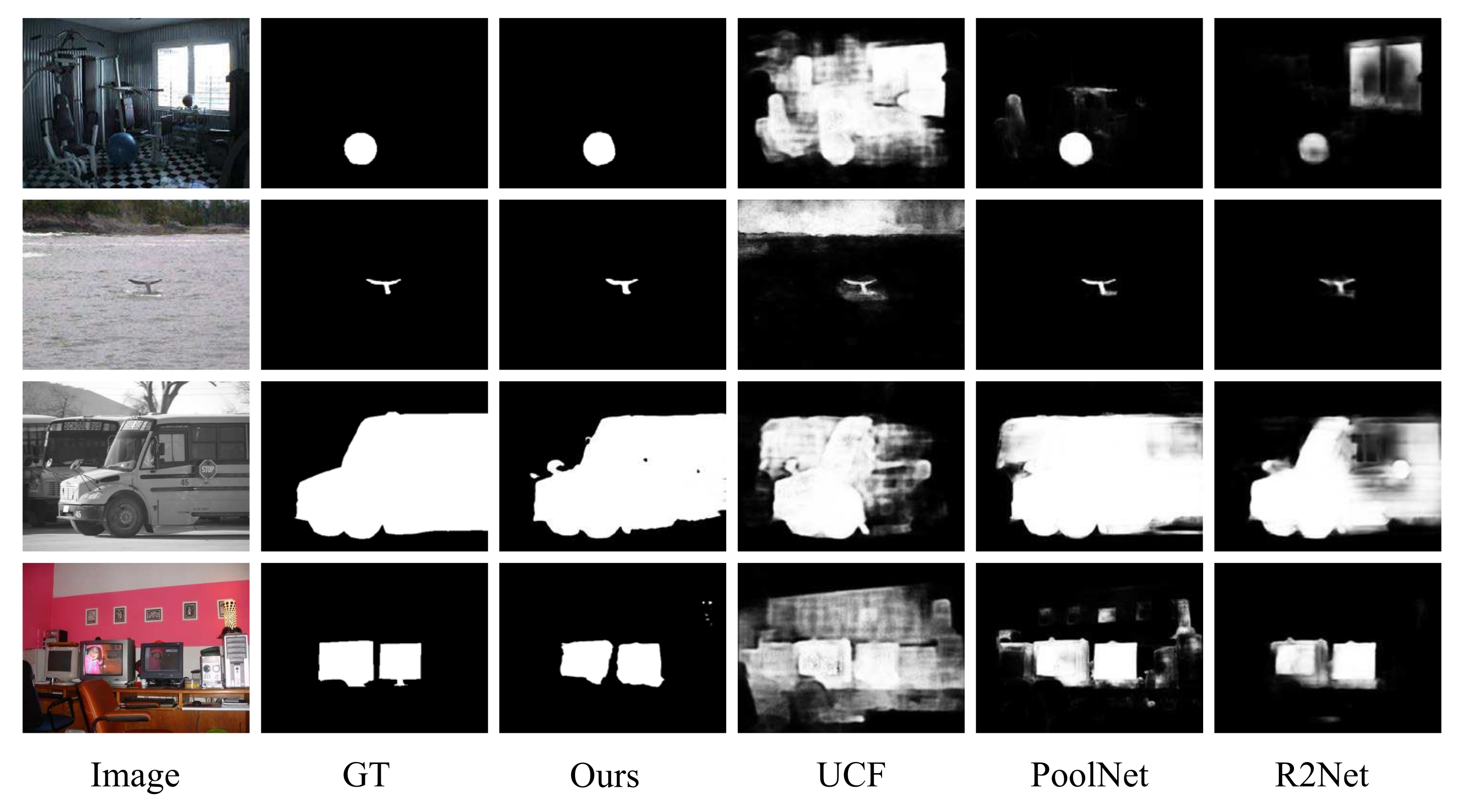
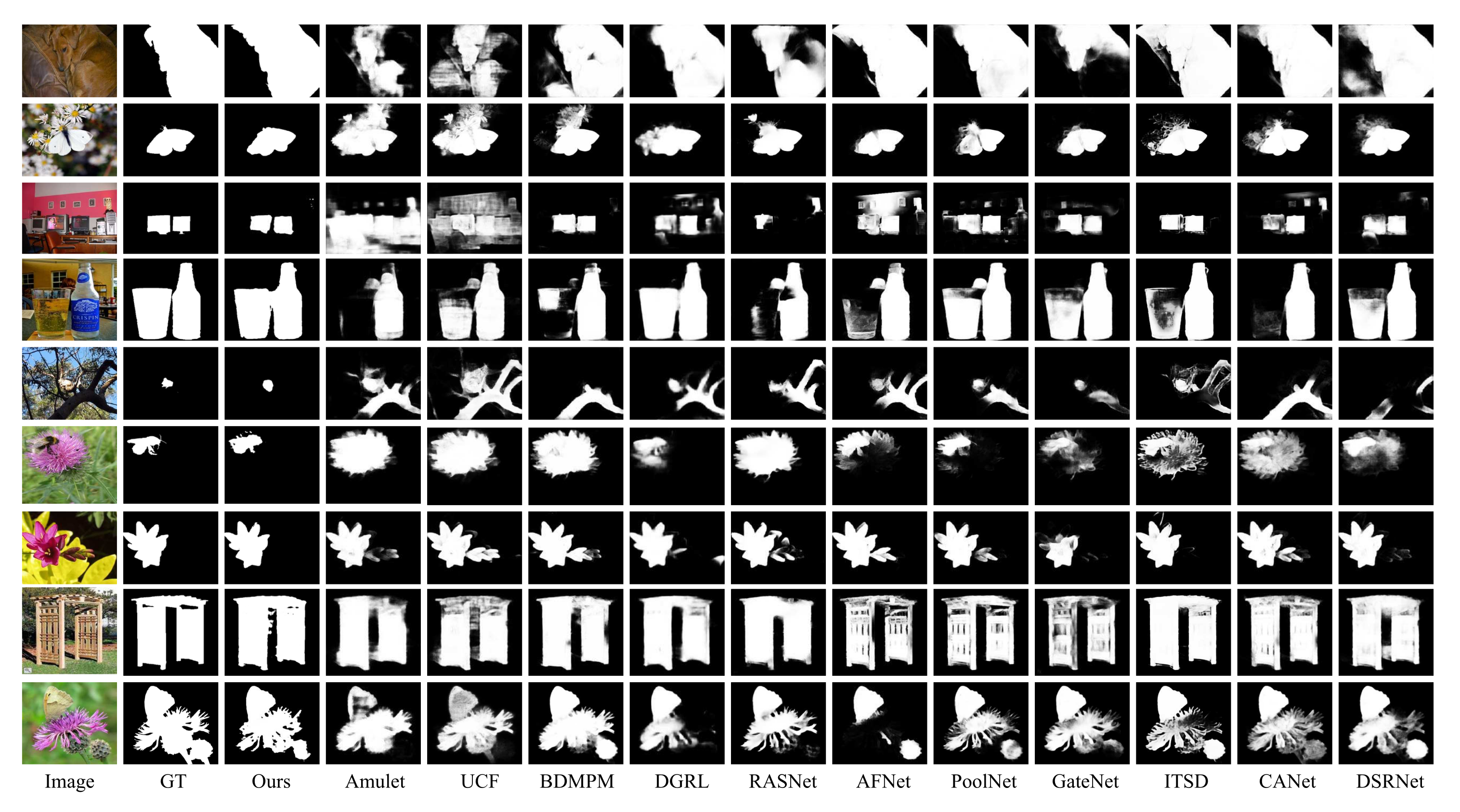
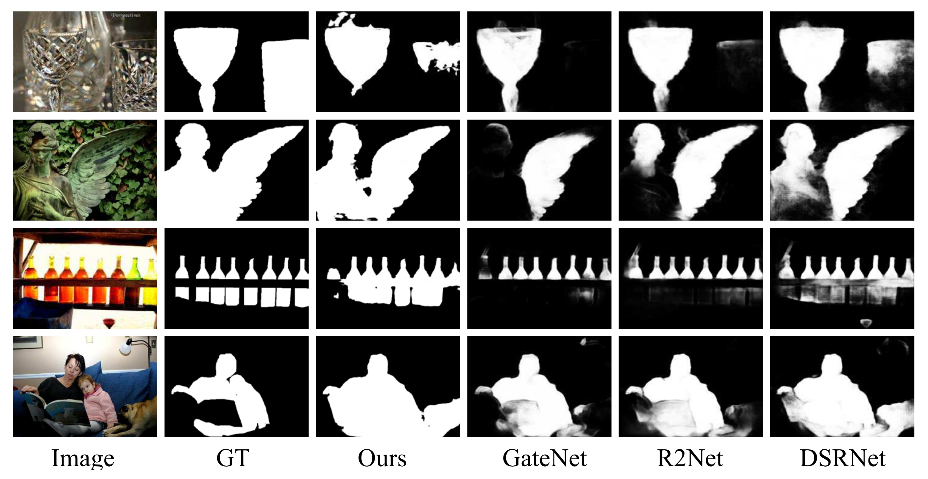
4.4.2. Qualitative Evaluation

Figure 7 shows visual comparisons of the proposed method with 11 state-of-the-art SOD methods. It can be inferred that the saliency maps in different scenarios generated by the proposed GSCINet method are much closer to the ground truth (GT). In contrast, most of the SOTA methods fail to consistently obtain satisfying results, especially in some challenging scenarios, including salient objects with low contrast or similar contours to the background (rows 1 and 2), multiple salient objects of the same semantic (rows 3 and 4), smaller salient objects in complicated environments (rows 5 and 6), and salient objects with big contour structures (rows 7, 8, and 9). More importantly, our method can detect and segment the complete salient objects with sharp boundaries, while most of the other methods produce the under-segmented saliency maps, demonstrating the effectiveness of the proposed GSCINet method.

4.4.3. Efficiency Evaluation

To further demonstrate the effectiveness of the proposed GSCINet method, we also evaluated the efficiency and flexibility of our model and some existing SOD methods, including the number of model parameters (#Param), the inference speed (FPS), and the model memory (M). From

Table 2. The proposed GSCINet method and other SOD methods in the comparison of parameter number (#Param (M)), inference Speed (FPS), and Model Memory (M).

Method	Input Size	#Param (M)	Inference Speed (FPS)	Model Memory (M)
Amulet	320 × 320	33.15	8	132
DGRL	384 × 384	161.74	8	631
BDMPM	256 × 256	-	22	259
AFNet	224 × 224	37.11	26	128
BASNet	256 × 256	87.06	25	332
PoolNet	384 × 384	68.26	17	410
R2Net	224 × 224	-	33	117
GateNet	384 × 384	128.63	30	503
DSRNet	400 × 400	75.29	15	290
CANet	256 × 256	-	32	-
Ours	320 × 320	24.46	40	96

, we identified that the inference time of our DSCINet achieved a speed of 40 FPS without any other post-processing, which is very competitive compared with the other methods. Furthermore, the number of model parameters and the size of model memory of the proposed GSCINet are 24.46 and 96, respectively, which are much smaller compared with the other SOD methods. These results further show the superiority of our GSCINet method in the efficient and accurate detection of salient objects.

4.5. Ablation Studies

The proposed GSCINet method consists of two modules, including a Multi-Scale Contextual Attention Module (MSCAM) and an Adjacent Feature Shrinkage and Interaction Module (AFSIM). To demonstrate the effectiveness of each component, we conducted a series of ablation studies on five public SOD benchmark datasets. Note that all ablation experiments were conducted with the ResNet-50 [34] backbone on five public SOD datasets, and the training strategies for all methods were the same in this section.

4.5.1. The Effectiveness of MSCAM

The MSCAM is designed to efficiently promote the saliency information of each initial multi-level feature by aggregating multi-scale and multi-receptive-field contextual attention features. To show the advantages of the MSCAM, we gave another three methods for comparison. The first method (named “Backbone”) only uses the ResNet-50 network [34] to detect and segment salient objects. The second method (named “Backbone+FPN”) uses the “Feature Pyramid Network (FPN)” [19] structure to generate saliency maps. The third method (named “Backbone+ASPP+FPN”) utilizes the “Atrous Spatial Pyramid Pooling (ASPP)” structure [48] to strengthen the performance of the initial multi-level features for SOD.

Table 3. Ablation analysis of our GSCINet method on ECSSD, PASCAL-S, HKU-IS, DUT-OMRON, and DUTS-TE datasets under four evaluation metrics. The symbols “↑/↓” indicate that the larger the result, the better, and the smaller the result, the better.

Method	ECSSD (1000)				PASCAL-S (850)				HKU-IS (4447)				DUT-OMRON (5168)				DUTS-TE (5019)
	$\mathbf{MAE}$↓	${\mathbf{AF}}_{\mathbf{m}}$↑	${\mathbf{WF}}_{\mathbf{m}}$↑	${\mathbf{E}}_{\mathbf{m}}$↑	$\mathbf{MAE}$↓	${\mathbf{AF}}_{\mathbf{m}}$↑	${\mathbf{WF}}_{\mathbf{m}}$↑	${\mathbf{E}}_{\mathbf{m}}$↑	$\mathbf{MAE}$↓	${\mathbf{AF}}_{\mathbf{m}}$↑	${\mathbf{WF}}_{\mathbf{m}}$↑	${\mathbf{E}}_{\mathbf{m}}$↑	$\mathbf{MAE}$↓	${\mathbf{AF}}_{\mathbf{m}}$↑	${\mathbf{WF}}_{\mathbf{m}}$↑	${\mathbf{E}}_{\mathbf{m}}$↑	$\mathbf{MAE}$↓	${\mathbf{AF}}_{\mathbf{m}}$↑	${\mathbf{WF}}_{\mathbf{m}}$↑	${\mathbf{E}}_{\mathbf{m}}$↑
Backbone	0.055	0.877	0.853	0.915	0.084	0.779	0.751	0.858	0.043	0.864	0.842	0.932	0.070	0.690	0.654	0.769	0.053	0.766	0.740	0.885
Backbone+FPN	0.045	0.891	0.880	0.930	0.070	0.805	0.787	0.877	0.038	0.875	0.862	0.946	0.058	0.727	0.703	0.864	0.045	0.795	0.781	0.906
Backbone+AFSIM	0.041	0.909	0.894	0.942	0.067	0.827	0.806	0.897	0.032	0.897	0.886	0.950	0.055	0.744	0.722	0.857	0.040	0.829	0.815	0.917
Backbone+ASPP+FPN	0.039	0.908	0.896	0.945	0.067	0.814	0.795	0.888	0.034	0.884	0.872	0.948	0.056	0.738	0.718	0.862	0.042	0.809	0.796	0.912
Backbone+MSCAM+FPN	0.039	0.917	0.908	0.946	0.065	0.823	0.804	0.884	0.030	0.907	0.896	0.956	0.055	0.761	0.740	0.870	0.039	0.834	0.823	0.918
Backbone+MSCAM+AFSIM	0.034	0.923	0.911	0.953	0.064	0.831	0.811	0.898	0.029	0.910	0.900	0.957	0.054	0.757	0.736	0.862	0.038	0.838	0.823	0.920

shows the result of quantitative comparisons. Specifically, the “Backbone+MSCAM+FPN”(the 5th row) consistently outperforms the “Backbone” (the 1st row ) and “Backbone+FPN”(the 2nd row ) with a margin of (6.80% and 3.18%), (7.06% and 2.16%), (6.41% and 3.94%), (13.15% and 5.26%), and (11.22% and 5.38%) on ECSSD, PASCAL-S, HKU-IS, DUT-OMRON, and DUTS-TE datasets, $w.r.t$, $W{F}_m$. Furthermore, the predicted performance of MSCAM is significantly improved in other evaluation metrics. In addition, by comparing the “Backbone+ASPP+FPN” (the 4th row ), the only addition of our MSCAM in the ResNet50 backbone network clearly brings performance gain under the four evaluation metrics (as illustrated in Figure 8). Therefore, it can be concluded that the proposed MSCAM is effective in location and segmentation of the salient objects, whose performance clearly outperforms the “Backbone”, “Backbone+FPN”, and “Backbone+ASPP+FPN” methods, receptively.

4.5.2. The Effectiveness of AFSIM

The AFSIM can progressively reduce the amount of calculations to improve inference speed and training efficiency, which can adaptively interact with diverse information on multi-level features to generate powerful and robust feature representations for accurate and efficient SOD. As observed in Table 3, compared with “Backbone” and “Backbone+FPN”, the proposed AFSIM can enhance the ability to detect salient objects in challenging scenes. Specifically, 0.909 vs. 0.877 and 0.891, 0.827 vs. 0.805 and 0.779, 0.897 vs. 0.864 and 0.875, 0.744 vs. 0.690 and 0.727, and 0.829 vs. 0.766 and 0.795 on the public SOD benchmark datasets in terms of $A{F}_m$. Furthermore, the other three evaluation metrics (i.e., $MAE$, $W{F}_m$ and $E_m$) also achieve great promotion (as depicted in Figure 8), proving the effectiveness of the proposed AFSIM. In addition, as depicted in Table 3, it can be seen that the sixth row (w MSCAM and AFSIM) significantly improves the prediction performance compared with third (w AFSIM) and fifth (w MSCAM) rows. Specifically, the $MAE$ scores of our GSCINet method are respectively reduced by (20.59% and 5.88%), (4.69% and 1.56%), (10.35% and 3.45%), (1.85% and 1.85%), and (5.26% and 2.63%). Similarly, the performance of the other three evaluation metrics also increased. These results demonstrate the effectiveness of the proposed MSCAM and AFSIM when inserted into the backbone network simultaneously.

4.6. Analysis and Limitations

Although the proposed GSCINet method has accomplished satisfactory results, it still has some limitations. Some failure examples are shown in Figure 9. When the images have low contrast objects and backgrounds (the top two rows), it is challenging for the proposed DSCINet method. Nevertheless, it is also tricky for state-the-of-art SOD methods (e.g., GateNet [22], R2Net [21], and DSRNet [30]). Furthermore, for the images with objects obscured by background (the third and fourth rows), the proposed GSCINet method also fails to predict satisfactory saliency maps. Hence, more different information is required to help capture distinguishing objects.

In future work, we will take into account multi-modal information (e.g., depth information, text information) to further strengthen the expressive ability of multi-level features, thereby generating high-quality representations for accurate and efficient SOD tasks. In addition, we will explore some questions about the influence of emotion and brain memory on locating salient objects in real-world scenes.

5. Conclusions

In this paper, we proposed a novel Gradual Shrinkage and Cyclic Interaction Network, namely GSCINet, which aims to discriminate more saliency information at the cost of fewer parameters and calculations for efficient and accurate SOD. This method was implemented with two essential modules, i.e., MSCAM and AFSIM. The former substantially increases the valuable information of initial input features by using a series of light-weight and multi-receptive-field dilated convolutions and embedding multiple attention weight matrices. The latter emphasizes compressing and optimizing the multi-level features via adaptively aggregating adjacent features and using a circular interaction strategy. The collaboration of MSCAM and AFSIM is able to progressively filter out background noise and enhance the information of salient objects. Extensive experimental results on five public SOD datasets demonstrate that our GSCINet method significantly outperforms 17 state-of-the-art saliency detection methods under different evaluation metrics.

References

1. He, J.; Feng, J.; Liu, X.; Cheng, T.; Lin, T.H.; Chung, H.; Chang, S.F. Mobile product search with bag of hash bits and boundary reranking. In Proceedings of the IEEE Conference on Computer Vision and Pattern Recognition (CVPR), Providence, RI, USA, 16–21 June 2012; pp. 3005–3012. [Google Scholar]
2. Zhang, P.; Zhuo, T.; Huang, W.; Chen, K.; Kankanhalli, M. Online object tracking based on CNN with spatial-temporal saliency guided sampling. Neurocomputing 2017, 257, 115–127. [Google Scholar] [CrossRef]
3. Cheng, M.M.; Liu, X.C.; Wang, J.; Lu, S.P.; Lai, Y.K.; Rosin, P.L. Structure-preserving neural style transfer. IEEE Trans. Image Process. 2019, 29, 909–920. [Google Scholar] [CrossRef] [PubMed] [Green Version]
4. Guo, C.; Zhang, L. A Novel Multiresolution Spatiotemporal Saliency Detection Model and Its Applications in Image and Video Compression. IEEE Trans. Image Process. 2010, 19, 185–198. [Google Scholar] [PubMed]
5. Margolin, R.; Tal, A.; Zelnik-Manor, L. What Makes a Patch Distinct? In Proceedings of the IEEE Conference on Computer Vision and Pattern Recognition (CVPR), Portland, OR, USA, 23–28 June 2013; pp. 1139–1146. [Google Scholar]
6. Klein, D.A.; Frintrop, S. Center-surround divergence of feature statistics for salient object detection. In Proceedings of the IEEE International Conference on computer vision (ICCV), Barcelona, Spain, 6–13 November 2011; pp. 2214–2219. [Google Scholar]
7. Cheng, M.M.; Mitra, N.J.; Huang, X.; Torr, P.H.; Hu, S.M. Global contrast based salient region detection. IEEE Trans. Pattern Anal. Mach. Intell. 2014, 37, 569–582. [Google Scholar] [CrossRef] [PubMed] [Green Version]
8. Xia, C.; Gao, X.; Fang, X.; Li, K.C.; Su, S.; Zhang, H. RLP-AGMC: Robust label propagation for saliency detection based on an adaptive graph with multiview connections. Signal Process. Image Commun. 2021, 98, 116372. [Google Scholar] [CrossRef]
9. Xia, C.; Zhang, H.; Gao, X.; Li, K. Exploiting background divergence and foreground compactness for salient object detection. Neurocomputing 2020, 383, 194–211. [Google Scholar] [CrossRef]
10. Wang, L.; Lu, H.; Ruan, X.; Yang, M.H. Deep networks for saliency detection via local estimation and global search. In Proceedings of the IEEE Conference on Computer Vision and Pattern Recognition (CVPR), Boston, MA, USA, 7–12 June 2015; pp. 3183–3192. [Google Scholar]
11. Zhao, R.; Ouyang, W.; Li, H.; Wang, X. Saliency detection by multi-context deep learning. In Proceedings of the IEEE Conference on Computer Vision and Pattern Recognition (CVPR), Boston, MA, USA, 7–12 June 2015; pp. 1265–1274. [Google Scholar]
12. Zhang, P.; Wang, D.; Lu, H.; Wang, H.; Yin, B. Learning uncertain convolutional features for accurate saliency detection. In Proceedings of the IEEE International Conference on Computer Vision (ICCV), Venice, Italy, 22–29 October 2017; pp. 212–221. [Google Scholar]
13. Zhang, L.; Dai, J.; Lu, H.; He, Y.; Wang, G. A Bi-Directional Message Passing Model for Salient Object Detection. In Proceedings of the IEEE Conference on Computer Vision and Pattern Recognition (CVPR), Salt Lake City, UT, USA, 18–23 June 2018; pp. 1741–1750. [Google Scholar]
14. Wang, T.; Zhang, L.; Wang, S.; Lu, H.; Yang, G.; Ruan, X.; Borji, A. Detect Globally, Refine Locally: A Novel Approach to Saliency Detection. In Proceedings of the IEEE Conference on Computer Vision and Pattern Recognition (CVPR), Salt Lake City, UT, USA, 18–23 June 2018; pp. 3127–3135. [Google Scholar]
15. Feng, M.; Lu, H.; Ding, E. Attentive Feedback Network for Boundary-Aware Salient Object Detection. In Proceedings of the IEEE Conference on Computer Vision and Pattern Recognition (CVPR), Long Beach, CA, USA, 19–20 June 2019; pp. 1623–1632. [Google Scholar]
16. Qin, X.; Zhang, Z.; Huang, C.; Gao, C.; Dehghan, M.; Jagersand, M. BASNet: Boundary-Aware Salient Object Detection. In Proceedings of the IEEE Conference on Computer Vision and Pattern Recognition (CVPR), Long Beach, CA, USA, 19–20 June 2019; pp. 7471–7481. [Google Scholar]
17. Ren, G.; Dai, T.; Barmpoutis, P.; Stathaki, T. Salient object detection combining a self-attention module and a feature pyramid network. Electronics 2020, 9, 1702. [Google Scholar] [CrossRef]
18. Da, Z.; Gao, Y.; Xue, Z.; Cao, J.; Wang, P. Local and Global Feature Aggregation-Aware Network for Salient Object Detection. Electronics 2022, 11, 231. [Google Scholar] [CrossRef]
19. Lin, T.Y.; Dollár, P.; Girshick, R.; He, K.; Hariharan, B.; Belongie, S. Feature pyramid networks for object detection. In Proceedings of the IEEE Conference on Computer Vision and Pattern Recognition (CVPR), Honolulu, HI, USA, 21–26 July 2017; pp. 2117–2125. [Google Scholar]
20. Liu, J.J.; Hou, Q.; Cheng, M.M.; Feng, J.; Jiang, J. A Simple Pooling-Based Design for Real-Time Salient Object Detection. In Proceedings of the IEEE Conference on Computer Vision and Pattern Recognition (CVPR), Long Beach, CA, USA, 19–20 June 2019; pp. 3912–3921. [Google Scholar]
21. Feng, M.; Lu, H.; Yu, Y. Residual Learning for Salient Object Detection. IEEE Trans. Image Process. 2020, 29, 4696–4708. [Google Scholar] [CrossRef] [PubMed]
22. Zhao, X.; Pang, Y.; Zhang, L.; Lu, H.; Zhang, L. Suppress and Balance: A Simple Gated Network for Salient Object Detection. In Proceedings of the European Conference on Computer Vision (ECCV), Amsterdam, The Netherlands, 8–16 October 2020; pp. 35–51. [Google Scholar]
23. Mei, H.; Liu, Y.; Wei, Z.; Zhou, D.; Xiaopeng, X.; Zhang, Q.; Yang, X. Exploring dense context for salient object detection. IEEE Trans. Circuits Syst. Video Technol. 2022, 32, 1378–1389. [Google Scholar] [CrossRef]
24. Tong, N.; Lu, H.; Zhang, L.; Ruan, X. Saliency detection with multi-scale superpixels. IEEE Signal Process. Lett. 2014, 21, 1035–1039. [Google Scholar]
25. Zhang, P.; Wang, D.; Lu, H.; Wang, H.; Ruan, X. Amulet: Aggregating Multi-level Convolutional Features for Salient Object Detection. In Proceedings of the IEEE International Conference on Computer Vision (ICCV), Venice, Italy, 22–29 October 2017; pp. 202–211. [Google Scholar]
26. Li, J.; Pan, Z.; Liu, Q.; Wang, Z. Stacked U-Shape Network With Channel-Wise Attention for Salient Object Detection. IEEE Trans. Multimed. 2021, 23, 1397–1409. [Google Scholar] [CrossRef]
27. Peng, H.; Li, B.; Ling, H.; Hu, W.; Xiong, W.; Maybank, S.J. Salient object detection via structured matrix decomposition. IEEE Trans. Pattern Anal. Mach. Intell. 2016, 39, 818–832. [Google Scholar] [CrossRef] [PubMed] [Green Version]
28. Borji, A.; Cheng, M.M.; Hou, Q.; Jiang, H.; Li, J. Salient object detection: A survey. Comput. Vis. Media 2019, 5, 117–150. [Google Scholar] [CrossRef] [Green Version]
29. Sina, M.; Mehrdad, N.; Ali, B.; Sina, G.; Mohammad, H. CAGNet: Content-Aware Guidance for Salient Object Detection. Pattern Recognit. 2020, 103, 107303. [Google Scholar]
30. Wang, L.; Chen, R.; Zhu, L.; Xie, H.; Li, X. Deep Sub-Region Network for Salient Object Detection. IEEE Trans. Circuits Syst. Video Technol. 2021, 31, 728–741. [Google Scholar] [CrossRef]
31. Long, J.; Shelhamer, E.; Darrell, T. Fully convolutional networks for semantic segmentation. In Proceedings of the IEEE Conference on Computer Vision and Pattern Recognition (CVPR), Boston, MA, USA, 7–12 June 2015; pp. 3431–3440. [Google Scholar]
32. Wu, Z.; Su, L.; Huang, Q. Cascaded Partial Decoder for Fast and Accurate Salient Object Detection. In Proceedings of the IEEE Conference on Computer Vision and Pattern Recognition (CVPR), Long Beach, CA, USA, 19–20 June 2019; pp. 3902–3911. [Google Scholar]
33. Ren, Q.; Lu, S.; Zhang, J.; Hu, R. Salient Object Detection by Fusing Local and Global Contexts. IEEE Trans. Multimed. 2021, 23, 1442–1453. [Google Scholar] [CrossRef]
34. He, K.; Zhang, X.; Ren, S.; Sun, J. Deep Residual Learning for Image Recognition. In Proceedings of the IEEE Conference on Computer Vision and Pattern Recognition (CVPR), Las Vegas, NV, USA, 27–30 June 2016; pp. 770–778. [Google Scholar]
35. Hou, Q.; Cheng, M.M.; Hu, X.; Borji, A.; Tu, Z.; Torr, P.H.S. Deeply Supervised Salient Object Detection with Short Connections. IEEE Trans. Pattern Anal. Mach. Intell. 2019, 41, 815–828. [Google Scholar] [CrossRef] [PubMed] [Green Version]
36. De Boer, P.T.; Kroese, D.P.; Mannor, S.; Rubinstein, R.Y. A tutorial on the cross-entropy method. Ann. Oper. Res. 2005, 134, 19–67. [Google Scholar] [CrossRef]
37. Máttyus, G.; Luo, W.; Urtasun, R. Deeproadmapper: Extracting road topology from aerial images. In Proceedings of the IEEE International Conference on Computer Vision (ICCV), Venice, Italy, 22–29 October 2017; pp. 3438–3446. [Google Scholar]
38. Yan, Q.; Xu, L.; Shi, J.; Jia, J. Hierarchical Saliency Detection. In Proceedings of the IEEE Conference on Computer Vision and Pattern Recognition (CVPR), Portland, OR, USA, 23–28 June 2013; pp. 1155–1162. [Google Scholar]
39. Li, Y.; Hou, X.; Koch, C.; Rehg, J.M.; Yuille, A.L. The Secrets of Salient Object Segmentation. In Proceedings of the IEEE Conference on Computer Vision and Pattern Recognition (CVPR), Columbus, OH, USA, 23–28 June 2014; pp. 280–287. [Google Scholar]
40. Li, G.; Yu, Y. Visual saliency based on multiscale deep features. In Proceedings of the IEEE Conference on Computer Vision and Pattern Recognition (CVPR), Boston, MA, USA, 7–12 June 2015; pp. 5455–5463. [Google Scholar]
41. Yang, C.; Zhang, L.; Lu, H.; Ruan, X.; Yang, M.H. Saliency Detection via Graph-Based Manifold Ranking. In Proceedings of the IEEE Conference on Computer Vision and Pattern Recognition (CVPR), Portland, OR, USA, 23–28 June 2013; pp. 3166–3173. [Google Scholar]
42. Wang, L.; Lu, H.; Wang, Y.; Feng, M.; Wang, D.; Yin, B.; Ruan, X. Learning to Detect Salient Objects with Image-Level Supervision. In Proceedings of the IEEE Conference on Computer Vision and Pattern Recognition (CVPR), Honolulu, HI, USA, 21–26 July 2017; pp. 3796–3805. [Google Scholar]
43. Achanta, R.; Hemami, S.; Estrada, F.; Susstrunk, S. Frequency-tuned salient region detection. In Proceedings of the IEEE International Conference on Computer Vision (ICCV), Kyoto, Japan, 29 September–2 October 2009; pp. 1597–1604. [Google Scholar]
44. Fan, D.P.; Gong, C.; Cao, Y.; Ren, B.; Cheng, M.M.; Borji, A. Enhanced-alignment Measure for Binary Foreground Map Evaluation. In Proceedings of the International Joint Conference on Artificial Intelligence, Stockholm, Sweden, 13–19 July 2018; pp. 698–704. [Google Scholar]
45. Chen, S.; Tan, X.; Wang, B.; Hu, X. Reverse attention for salient object detection. In Proceedings of the European conference on computer vision (ECCV), Munich, Germany, 8–14 September 2018; pp. 234–250. [Google Scholar]
46. Liu, Y.; Zhang, Q.; Zhang, D.; Han, J. Employing deep part-object relationships for salient object detection. In Proceedings of the IEEE International Conference on computer vision (ICCV), Seoul, Korea, 27 October–2 November 2019; pp. 1232–1241. [Google Scholar]
47. Zhou, H.; Xie, X.; Lai, J.H.; Chen, Z.; Yang, L. Interactive Two-Stream Decoder for Accurate and Fast Saliency Detection. In Proceedings of the IEEE Conference on Computer Vision and Pattern Recognition (CVPR), Seattle, WA, USA, 13–19 June 2020; pp. 9138–9147. [Google Scholar]
48. Chen, L.C.; Papandreou, G.; Schroff, F.; Adam, H. Rethinking atrous convolution for semantic image segmentation. arXiv 2017, arXiv:1706.05587. [Google Scholar]
Figure 1. Illustration for saliency maps of the proposed GSCINet methods compared with other FPN-based SOD methods, including UCF [12], PoolNet [20] and R2Net [21]. Note that GT denotes ground truth.
Electronics 11 01964 g001
Figure 2. Illustration of different network structures. Left to right column: Feature Pyramid Network (FPN) [19] and Our GSCINet Network structures are depicted, respectively.
Electronics 11 01964 g002
Figure 3. The complete architecture of the proposed GSCINet method for fast and accurate salient object detection, consisting of a Multi-Scale Contextual Attention Module (MSCAM) and an Adjacent Feature Shrinkage and Interaction Module (AFSIM).
Electronics 11 01964 g003
Figure 4. Detailed illustration of the proposed Multi-Scale Contextual Attention Module (MSCAM).
Electronics 11 01964 g004
Figure 5. Quantitative results of P R curves for GSCINet and other SOD methods on the five saliency detection datasets.
Electronics 11 01964 g005
Figure 6. Quantitative results of F m curves for GSCINet and other SOD methods on the five saliency detection datasets.
Electronics 11 01964 g006
Figure 7. Qualitative comparison of 11 state-of-the-art deep SOD methods and our GSCINet method. As can be seen, the proposed method (ours) is the closest to ground truth (GT).
Electronics 11 01964 g007
Figure 8. Ablation studies results of the proposed GSCINet method. The five points denote “Backbone”, “Backbone+FPN”, “Backbone+AFSIM”, “Backbone+MSCAM+FPN”, and “Backbone+MSCAM+AFSIM”, respectively.
Electronics 11 01964 g008aElectronics 11 01964 g008b
Figure 9. Failure cases of the proposed GSCINet method and other state-of-the-art SOD methods, including GateNet [22], R2Net [21] and DSRNet [30].
Electronics 11 01964 g009