Digital Forensics Classification Based on a Hybrid Neural Network and the Salp Swarm Algorithm

Abstract

In recent times, cybercrime has increased significantly and dramatically. This made the need for Digital Forensics (DF) urgent. The main objective of DF is to keep proof in its original state by identifying, collecting, analyzing, and evaluating digital data to rebuild past acts. The proof of cybercrime can be found inside a computer’s system files. This paper investigates the viability of Multilayer perceptron (MLP) in DF application. The proposed method relies on analyzing the file system in a computer to determine if it is tampered by a specific computer program. A dataset describes a set of features of file system activities in a given period. These data are used to train the MLP and build a training model for classification purposes. Identifying the optimal set of MLP parameters (weights and biases) is a challenging matter in training MLPs. Using traditional training algorithms causes stagnation in local minima and slow convergence. This paper proposes a Salp Swarm Algorithm (SSA) as a trainer for MLP using an optimized set of MLP parameters. SSA has proved its applicability in different applications and obtained promising optimization results. This motivated us to apply SSA in the context of DF to train MLP as it was never used for this purpose before. The results are validated by comparisons with other meta-heuristic algorithms. The SSAMLP-DF is the best algorithm because it achieves the highest accuracy results, minimum error rate, and best convergence scale.

1. Introduction

Great technological development has led to the use of the Internet in many areas of life [1]. Many companies have taken advantage of the Internet to provide many services using e-commerce without having to submit to market restrictions. This reflected positively in the country’s economy by increasing competitiveness and achieving great returns. This has caused a huge positive shift in the number of customers who use the Internet to buy, sell, and transfer large amounts of money [2]. These large sums are tempting for many hackers and scammers to engage in many activities that violate privacy. These put a lot of people and companies at risk through the web and cause huge financial losses [3]. Other violations that may occur online include impersonation, loss of privacy, brand theft, and loss of customers’ trust in institutions. Hence, the suitability of the Internet for carrying out business and banking operations is called into question.

DF is a direct result of cybercrime, which is typically applied in computer-related crimes [4,5,6]. This includes Intellectual property infringement, use of unauthorized privileges to deal with the computer systems, privacy infringement, a security breach of confidential data repositories, carrying out terrorist operations via the Internet, misuse of electronic data, etc. DF is defined as an organized process that uses scientific techniques to collect, document, and analyze electronically stored data. This helps utilize the computer equipment and storage media to provide evidence to detect the abnormal events [7].

Suspicious events and unsafe activities may lead organizations to lose a lot of money, in addition to losing their prestige. Therefore, such events may lead to serious repercussions for both individuals and institutions. According to the statistics shown by the published reports, the number of computer violations has reached more than five million violations so far [8]. Many cybercrimes go unrecorded because their victims do not report them to officials. Victims of cybercrime feel confused and humiliated or believe that the authorities are not taking the necessary measures to punish the attackers. In addition to the lack of competencies and expertise from the workforce, the government needs to mitigate computer crimes [9].

Crime scene cyber investigations include conducting forensic analysis of all types of storage and digital media increasing the volume of data obtained. The value of data depends on the extent to which it is used in decision-making. The process of analyzing digital data during forensic practice is traditionally manual in most cases. Investigators perform reports using some statistical tools to give a picture of the collected data [10]. However, the cost of digital investigations increases with increasing data dimensions. Furthermore, forensic cases increase the data analysis complexity, which leads to the deterioration of the manual process quickly [11]. It is necessary to use more advanced methods with potential beyond the capacity of the conventional manual analysis in dealing with big data. Machine learning (ML) is an efficient and more sophisticated method that facilitates the production of useful knowledge for decision-makers. This is carried out by analyzing data sets from different perspectives and fixing them into meaningful forms [12].

The primary goal of DF analysis is to identify who is responsible for these cyber security crimes. This is performed by the selection, classification, and reordering of the sequence of events of the digital crime. Acts reorganization analyzes DF and prepares a schedule of these cyber events. It determines digital evidence, which is information with true value gained from trusted sources that admit or do not admit to committing cybercrime. Over there, there are many sources from which reliable information can be collected to rebuild cybercrime events, such as web browsers, history files, cookies messages, temporary files, log files, and system files [13].

Some of the valuable sources of information that can aid the DF are the system files and their metadata. These files are normally modified by users and the usual use of computer machines. The reconstruction process for digital events can benefit from the system files affected by cyber-crime. However, these files may be modified by normal programs [14]. For this reason, the reconstruction of digital events and the determination of the timeline sequence of events and activities are essential. This helps to recognize whether the type of application that manipulates the file system is reliable or malicious.

The main problem to be solved in this paper is the classification of files that have been accessed, manipulated, changed, and deleted by application programs. This depends on using some features that are represented by footprints. Identifying the affected files by specious acts facilitates the process of event reconstruction in the file system.

This paper presents one of the Neural Network techniques for rebuilding the acts of a digital crime. Multi-layer perceptron (MLP) is one of the artificial neural networks (ANNs) that imitates the neural human system [15]. It has been used in many applications as a supervised classifier. The main advantage of MLP is that it can learn and tackle many complex problems with promising results in science and engineering. It can be adopted efficiently for either supervised or unsupervised learning. In addition, it has a large ability to tackle parallelism, fault tolerance, and robustness to noise. MLP has a great capacity to generalize as well.

The most common problems of gradient-based MLP are stagnation in local minima, a tendency to the starting values of its parameters, and slow convergence. Due to the local minima problem, several studies in the literature proposed different approaches to train MLP. Swarm-based algorithms have been widely used to train MLPs. These algorithms simulate the natural survival of animals such as the Gradient-Based Optimizer (GBO) [16], Slime mould algorithm (SMA) [17], Heap-based optimizer (HBO) [18], and Harris hawks optimization (HHO) [19]. However, the local minima problem still exists. Furthermore, based on the no-free-lunch theorem (NFL), there is no preference among swarm algorithms. The superiority of one swarm algorithm over another does not imply superiority in all applications. This means that there is no guarantee that it will perform similarly when applied to other optimization problems. These reasons motivated us to propose a new method to train MLPs using the SSA algorithm in the context of DF.

SSA  [20] is one effective meta-heuristic algorithm that belongs to a swarm-based family. It has a set of characteristics that motivated us to select it. First, it has a single parameter that decreases in an adaptive manner relative to the increasing iterations. Second, it performs an extensive exploration in the initial iterations then it adaptively switches to exploit the most promising areas of the search space. Third, SSA preserves the best-found solution so that it never loses the optimal solution. Fourth, follower salps change their locations adaptively following other members of the population, so it has the power to alleviate the local minima problem.

SSA has been implemented to solve different optimization problems. In [21], Yang proposed a memetic SSA (MSSA) with multiple independent salp chains. He aimed to make more exploration and exploitation. Another improvement was using a population-based regroup operation for coordination between different salp chains. The MSSA is applied for an efficient maximum power point tracking (MPPT) of PV systems. The results showed the output energy generated by MSSA in Spring in Hong Kong is 118.57%, which is greater than the other algorithms. In [22], the author integrated the SSA with the Ant Lion Optimization algorithm (ALO) for intrusion detection in IoT networks. The true positive rates reached 99.9% and with a minimal delay. In [20], the authors proposed a new phishing detection system using SSA. They aimed to increase the classification performance and reduce the number of features of the phishing system. Different transfer function (TF) families: S-TFs, V-TFs, X-TFs, U-TFs and Z-TFs were used to generate a binary version of the SSA. The results showed that BSSA with X-TFs obtained the best results. In [23], the target of the proposed approach was to reduce the number of symmetrical features and obtain a high accuracy after implementing three algorithms: particle swarm optimization (PSO), the genetic algorithm (GA), and SSA. The used datasets are the Koirala dataset. The proposed COVID-19 fake news detection model obtained a high accuracy (75.4%) and reduced the number of features to 303. In [24], the authors introduced four optimizations algorithms integrated with an MLP neural network, namely artificial bee colony (ABC-MLP), grasshopper optimization algorithm (GOA-MLP), shuffled frog leaping algorithm (SFLA-MLP), and SSA-MLP to approximate the concrete compressive strength (CSC) in civil engineering. The results show that SSA-MLP and GOA-MLP can be promising alternatives to laboratory and traditional CSC evaluative methods.

The main contributions can be summarized as follows:

• The integration of SSA with MLP assists it since it can professionally avoid local minima;
• The high speed of convergence of SSA helps reach the optimal MLP structure quickly;
• The proposed method achieves better results compared with other algorithms in terms of accuracy, error rate, and convergence curve;
• The proposed method can deal with different scenarios with varying complexity.

This paper has the following sections: Section 2 reviews some of the previous studies that investigate DF. Section 3 provides a description for MLP. Section 4 discusses the details of the new MLPSSA-DF method. Section 5 discusses the dataset, experiments, and results. Finally, Section 6 summarizes the findings of the whole paper.

2. Forensic’s Background

The initiation of the DF investigations depends on the presence of some indications on the computer system. There are several indications that a computer system has experienced suspicious incidents and is a victim of cybercrime [25].

Table 1. DF indications.

Computer System Part	Indication
Booting	Slow
Turn-off	Slow
Response	Slow
Data	Deleted or destroyed
Processes	Unknown processes run
Disk space	Low
Pop-up windows	Many unexpected
Battery	Drains quickly
Wi-Fi	Unstable connection
Blue Screen	Displayed many times

shows these indications.

The goal of conducting DF investigations is to answer a range of questions as quickly as possible. These include:

• What are the motives for cybercrime?
• Where is the cybercrime site?
• When did the suspicious act happen?
• What suspicious acts occurred on the computer that warrants the action Investigation?
• What is the application program or tool that was used in the execution of the cybercrime?

DF investigations rely heavily on system files because they provide accurate and important information about the sequence of events involved in cybercrimes [26]. At the end of the DF investigations comes the question about how the cybercrime occurred, and this question depends on the answer to all the previous questions.

In the past, a general rule was devised regarding potential digital evidence based on documentary evidence considered admissible in court [27]. These steps include earning, identification, assessing, and admission. Years later, a specific methodology was developed for cybercrime research [28]. This methodology is an approach to all the proposed models that have been followed so far and includes the following steps:

• Define;
• Preserve;
• Gather;
• Test;
• Analyze;
• Present;
• Check.

In [29], the authors expanded the model in [28] by including two additional steps, which are set up and approach strategies. The new model was called the abstract DF model. The additional two steps were carried out after the define step and before the preserving step. The setup step involves the tools that are used to deal with the suspicious acts. On the other hand, the approach step involves a formal strategy for investigating the effect on the technology and viewers. The problem with this model is that it is quite generic, and there is no clear method to test it.

Through the models that have been proposed in [27,28,29], we can say that the steps of the DF are compatible with the steps of machine learning. In general, a DF investigation relies heavily on reconstructing events and preparing accurate evidence.

In [30], the authors devised a new method that initially requires the collection of evidence to reconstruct the acts, followed by the development of initial hypotheses. These hypotheses are studied, analyzed, and examined. From here begins the actual process of DF investigations. It ends with finding the outcomes of the electronic case. A new technique has been developed in [31] to reconstruct the latest acts. It is based primarily on defining the condemnation of data objects and the relationships between them.

In [32], the authors used an ant system to take the place on Grid hosts. The Ant-based Replication and Mapping Protocol (ARMAP) is used to spread resource information with a decentralized technique, and its performance is assessed using an entropy index. The authors in [33] developed a new method to reconstruct acts. It uses a finite state machine. It shows the transition from one state to another based on some conditions put by the evidence. In [34], the authors proposed ontology for reconstructing acts by representing the acts as entities. The events are represented by developing a time model to show the instance change in the state instead of using a period. The shellbag-based technique was proposed in [35], which preserves information in the Windows Registry. This information is about the files, folders, and windows that appear, such as deleted, modified, and relocated files and folders.

Nowadays, many tools are used to collect acts and save them in a temporal repository. However, it can be difficult to analyze the raw data.

In [36], Hall investigated the potential of EXplainable artificial intelligence (XAI) to enhance the analysis of DF evidence using examples of the current state of the art as a starting point. Bhavsar [37] pointed out the challenges in this forensics standard to design the framework of the investigation process for criminal activities using the best digital forensic instruments. Dushyant [38] discussed the advantages and disadvantages of incorporating machine learning and deep learning into cybersecurity to protect systems from unwanted threats. In [39], Casino conducted a review of all the relevant reviews in the field of digital forensics. The main challenges are related to evidence acquisition and pre-processing, collecting data from devices, the cloud, etc.

Unlike previous studies in the literature, where the proposed algorithm was trained on general datasets or limited applications, the newly developed MLP-SSA is proposed for the first time in the context of DF. Different evaluations are performed to test the viability of the MLPSSA to be used as a robust classifier for DF.

3. DF Using MLP

The MLP neural network can be used for the classification of files that have been accessed, manipulated, changed, and deleted by application programs. Once act depends on using some features that are represented by footprints. Identifying the affected files by specious acts facilitates the process of event reconstruction in the file system.

3.1. Dataset

The dataset used in the experiments is collected from three resources: the audit log, file system, and registry. It ensures that if some features are missed in one resource, they may be found in another resource. The dataset represents a database for the collected features of the system file or the metadata. The record contains the values of the files’ features that have been affected by a specific program. These are the footprints that are specific for each application program. It describes the system events or acts or metadata. As in supervised classification, the dataset has one column for class. In this dataset, the last column is the application program.

The collection of the features related to the system file using an application program is carried out using some programs such as the .Net program. This paper runs a program called VMware, which is used for collecting the features and building a training dataset. The main advantage of VMware is that it can get red from the useless programs and reduce their effects. The operating system used in this experiment is Windows 7 as it is a commonly used platform. The application programs used in the experiments are Internet Explorer, Acrobat Reader, MS-Word, MS-Excel (Microsoft Office version 2007), and VLC media player.

These applications are performed in different ways. First, the applications are loaded separately. Thus, if one application is completely loaded and then closed, the other program is loaded after it. The main issue in this execution of programs is that they do not do anything in the file system except loading and closing. Second, the applications also are loaded and executed and then closed one by one. In this case, the first three applications perform one act, which is saving a file. The last application visit (www.msn.com accessed on 20 April 2022) website. Third, as the first and second execution, the applications are loaded separately. However, different acts are executed by each application.

The acts of the first three applications include saving files, opening files, and creating new files. However, the last application performs a set of acts that include visiting secured/unsecured websites and sending/receiving emails with/without attachments. Fourth, in this execution, the applications are executed at the same time as opposed to previous executions. As in execution three, different acts take place. The number of examples of records in a database is 23,887.

Table 2. The features in a dataset.

Feature Number	Feature Name	Feature Value Example
1	Filename-length	255 characters
2	Filenamespace	_user/
3	Object Id	$ObjId$
4	Original-Volume-Id	$94F8-9C08$
5	Domain-Id	$dds::domain::DomainParticipant(DOMAIN\_ID,qos\_provider.participan{t}_{q}os\left(\right))$
6	Original-Object-Id	40dff02fc9b4d4118f120090273fa9fc

shows the features on the dataset that is used to investigate the digital forensics.

3.2. Preparing a Dataset

The performance of a machine learning model is greatly affected by the dataset. Therefore, preparing a dataset is an important stage for developing efficient and reliable models. It enhances the generalizing process. Different issues have been applied to a dataset to preprocess it before using it in the learning algorithm. First, restructuring of the dataset by distributing the values into sets in such a way the feature’s states reduce.

Another important concern in this regard is that most machine learning algorithms deal with numerical values instead of text values. Therefore, in the used dataset, there is a need to assign numerical values to some feature values using the word2vect tool. Using this tool, an index is assigned to each word. Second, cleaning the dataset and git-rid of missing and outlier values. These have a positive impact on enhancing the generalization and generating less biased models. Third, normalizing the dataset by scaling the values of the features into a predefined range using the min-max method. This helps to deal with all features equally instead of making one feature overwhelm the others.

3.3. Salp Swarm Algorithm (SSA)

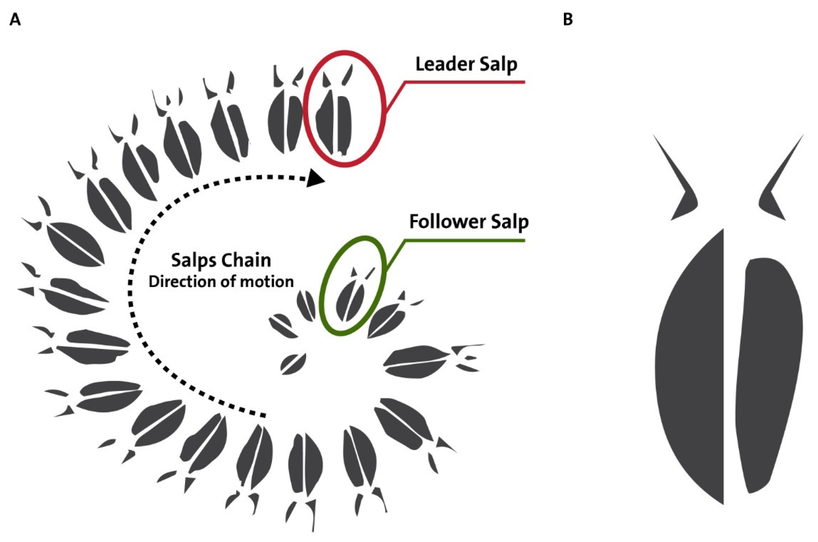
The inspiration for the SSA algorithm is from the salp aquatic animals. They have a specialized technique for obtaining food. The first salp in the swarm leads the other members in the sequence. This implies that other swarm members change their positions dynamically concerning the leader. Figure 1 shows a single salp on the right side and a swarm of salps on the left side.

Algorithm 1 (SSA) is an evolutionary algorithm that was developed by Mirjalili [20]. The swarm S of n salps can be represented in Equation (1), where $Foo$ is the source of food. The population of salps is represented by a matrix. Each row is a salp or solution. The length of the salp is the number of features in a dataset (d). The number of salps (n) is the swarm’s size. The first row in the matrix is the leader salp, and the other rows are for the follower salps.

$$S_i=\left[\begin{array}{cccc}{s}_1^1& s_2^1& \cdots & s_d^1\\ s_1^2& s_2^2& \cdots & s_d^2\\ ⋮& ⋮& ⋮& ⋮\\ s_1^n& s_2^n& \cdots & s_d^n\end{array}\right]$$

(1)

Equation (2) illustrates the location of the first salp

$$S_j^1=\left\{\begin{array}{c}Fo{o}_j+c{p}_1((up\_boun{d}_j-low\_boun{d}_j)c{p}_2\hfill \\ +low\_boun{d}_j),c{p}_3\ge 0.5\hfill \\ Fo{o}_j-c{p}_1((up\_boun{d}_j-low\_boun{d}_j)c{p}_2\hfill \\ +low\_boun{d}_j),c{p}_3<0.5\hfill \end{array}\right.$$

(2)

where $s_j^1$ and $Fo{o}_j$ are the locations of leader salp and the source of food in the $j_{th}$ dimension, respectively. In Equation (3), $c{p}_1$ gradually decreases and changes its value across cycles, and $curr$ and $last$ are the current and the last cycles, respectively. The other parameters $c{p}_2$ and $c_3$ in Equation (2) are randomly chosen from [0, 1]. $c{p}_2$ and $c{p}_3$ direct the next location in the $j_{th}$ dimension to +∞ or −∞ and determine the step size. The $up\_boun{d}_j$ and $low\_boun{d}_j$ are the limits of the $j_{th}$ dimension.

$$c{p}_1=2e^{-{\left(\frac{4curr}{last}\right)}^2}$$

(3)

$$S_j^i=\frac{1}{2}(s_j^i+s_j^{i-1})$$

(4)

In Equation (4), $i⩾2$, and $s_j^i$ is the location of the $i_{th}$ salp at the $j_{th}$ dimension.

Algorithm 1 SSA

In_variables: n is the size_swarm, d is the no_dimensions Out_variables: The best salp (Foo) Initial_variables s_i (i = 1, 2, . . . , n), up_bound and low_bound while (last cycle is not reached) do     Compute each salp’s fitness value     Determine Foo as the optimal salp     Update $c_1$ by Equation (3)     for (each salp $s_i$) do         if l == 1 then            Change the location of the first salp by Equation (2)         else            Change the locations of the other salps by Equation (4)         end if         Change the locations of the salps using the lower and upper bound     end for end while Return (F)

3.4. Multi-Layer Perceptron Neural Networks (MLP)

MLP is a type of feed-forward NN, which is used for training the data and discovering the hidden patterns in the training data. The pattern is then applied to the hidden instances of the dataset to obtain the results. Three layers are in the architecture of MLP: the first, the middle, and the last layers. Each layer consists of a set of computational nodes that simulate the human neurons. The MLP’s complexity increases by adding more middle layers. The standard MLP contains a single hidden layer. Figure 2 shows a standard MLP, with a first layer that has n nodes, a single middle layer that has m nodes, and a last layer that has k nodes.

The MLP can be visualized as a directed graph that connects the first layer with the middle layer and the middle layer with the last layer. Each middle node is connected with the first layer with n weights and with r weights with the last layer. In addition, there are m biases. The main processes that take place in the hidden nodes are the summation as in Equation (5) and the activation as in Equation (6). The output of Equation (5) of node m is performed using Equation (5). After computing the sum, a transfer function is applied to the input as in Equation (6).

$$SumFu{n}_m=\sum _{n=1}^n{d}_{nm}\ast P_n+c_m$$

(5)

where $d_{nm}$ is the weight between the first node $Pn$ and the middle node $hm$, and $c_m$ is the bias m that enters the middle node m.

$$o_m=Sig\left(SumFu{n}_m\right)$$

(6)

where $o_m$ is the output node m; $m=1,2,\cdots ,s$; $Sig$ is the sigmoid function as in Equation (7)

$$Sig\left(SumFu{n}_m\right)=\frac{1}{1+e^{-SumFu{n}_m}}$$

(7)

After collecting the results from all the m nodes, the final result $O_m$ can be generated as shown in Equations (8) and (9).

$$SumFu{n}_m=\sum _{n=1}^s{d}_{nm}\ast o_m+c_m$$

(8)

where $d_{nm}$ is the weight between the node n in the middle layer and the node m in the last layer, and $c_m$ is the bias m that enters to the output node m.

$$O_m=f\left(SumFu{n}_m\right)$$

(9)

where $O_m$ is the final result m; $m=1,2,\cdots ,r$; $Sig$ is the function applied in Equation (7).

4. SSAMLP-DF Model

MLP is a type of NN that uses the feed-forward NN architecture and backpropagation method to propagate data from input nodes to hidden nodes to output nodes. The following list shows the stages of the SSAMLP-DF model:

• Collecting data;
• Data pre-processing;
• MLP construction;
• MLP training phase;
• MLP testing phase.

There are many areas in which the MLP has been implemented. The main features of MLP that helped it to be commonly used include the nonlinear structure, adaptive update of its parameters, and the ability to generalize well compared with other algorithms. Initially, the dataset is divided into three parts: 70% to train the model, 15% to validate the model, and 15% to test the model and mitigate the overfitting problem. This is called the “Hold-Out” validation method. Overfitting is a popular machine learning problem in which the error rate in the training phase is too small, but it increases in the testing phase. Of course, this is not what is required.

The main target of MLP is to build an accurate model with a minimum error achieved in the testing phase. By applying the MLP to the training part of a dataset, the initial MLP structure is constructed. These include the MLP’s layers and the number of nodes in each middle layer. The weights of the MLP are set to nonzero values. MLP trains a model until a specific condition is satisfied, such as reaching the maximum number of cycles or achieving a threshold error rate. If the trainer achieves the stopping condition, then the weight parameters of the generated model are kept. If the stopping condition is not met, then the MLP structure is updated by changing the number of nodes in the middle layer.

The MLP structure has a large number of nodes in the middle layer and is then progressively resourced across cycles until an acceptable performance is achieved. This method is called the punning method, and it is used to determine the number of nodes in the middle layer that is suitable to generate the desired performance. After the model is generated, the testing dataset is applied to this model, and the error rate is approximated. The basic measurement is the accuracy, which is calculated by dividing the correctly classified instances by the total number of instances in the testing part of the dataset. It is computed as follows:

$$ACC\text{-}DF=\frac{TP\text{-}DF+TN\text{-}DF}{TP\text{-}DF+TN\text{-}DF+FP\text{-}DF+FN\text{-}DF}$$

(10)

where ($TP\text{-}DF$) is the number of files that are predicted to have tampered with a specific computer program, and it is tampered by a specific computer program. ($FN\text{-}DF$) is the number of files that are tampered by a specific computer program and incorrectly predicted that they are not tampered by a specific computer program. ($FP\text{-}DF$) is the number of files that are not tampered by a specific program and incorrectly predicted to be tampered by a specific program. ($TN\text{-}DF$) is the number of files that are not tampered by a specific program and incorrectly predicted to be not tampered by a specific program. The generated DF-model is trained using MATLAB.

This section presents the proposed DF model by integrating the SSA and MLP algorithms. In this model, the SSA is used to train the MLP based on one hidden layer. Two important issues must be taken into account: the representation of the solution in the SSA and the fitness function. Each solution is represented as a one-dimensional array and its values represent a candidate MLP structure. The solution in the SSA-MLP model is partitioned into three parts: the weight parameters that connect the input nodes with the hidden nodes, the weight parameters that connect the hidden nodes with the output nodes, and the biases. The solution’s length equals the number of connection weights in addition to the number of biases. Equation (11)

$$Solutio{n}^{\prime }slength=(P\times M)+(2\times M)+1$$

(11)

where P is the number of input nodes, and M is the the number of the hidden nodes.

The fitness value in the SSA-MLP model is the mean square error (MSE). This is calculated by subtracting the predicted value from the actual value by the generated solutions (MLPs) for the training part instances of the dataset. MSE is shown in Equation (12), where R is the actual value, $\widehat{R}$ is the value generated from prediction, and N is the number of examples in the training dataset.

$$MSE=\sum _{i=1}^N{(R-\widehat{R})}^2$$

(12)

The steps of the proposed SSA-MLP can be summarized as follows:

• The candidate individuals of the SSA are initialized randomly. These represent the possible solutions of the MLP.
• Evaluating the fitness of solutions. In this step, randomly generated values are assigned to the bits of solutions that represent the possible values of the connection weights and biases. These solutions are then assessed by the MLP. MSE is a popular function that is selected to evaluate the evolutionary-based MLP models. The main purpose of the training stage is to obtain the best network structure of the MLP that generates the minimum error rate or MSE value when implemented on a training part of the dataset
• Update each solution by changing the position of search agents in the SSA algorithm.
• Steps 2 and 3 are repeated until the stopping condition is satisfied. The last stage of the proposed model is generating the optimal MLP structure with the best weight parameters and biases. This MLP structure is tested on the testing and validation parts of the dataset. Therefore, the obtained error rate by MSE is the minimum. Figure 3 shows the assignment of a salp to MLP. Figure 4 shows the general steps of the proposed DF-SSA-MLP model.

5. Experiments and Results

This section presents the classification results of the proposed SSAMLP versus other metaheuristic algorithms in terms of accuracy. Twenty-four experiments were established to evaluate the different algorithms in terms of the accuracy of results using different MLP structures. Furthermore, an analysis of their convergence curves is illustrated. The proposed approach is compared against seven metaheuristic algorithms integrated with MLP using the same experiment specifications. These algorithms are: Particle Swarm Optimization (PSO) [40], Ant Colony Optimization (ACO) [41], Genetics Algorithm (GA) [42], Differential Evolution algorithm (DE) [43], and BackPropagation [44].

These experiments performed the proposed methods on 14 benchmark mathematical functions used for minimization problems.

Table 3. The parameters’ values for the applied algorithms.

Algo	Parameter	Val
SSA	c1	[0–1]
	c2	[0–1]
GA	CrossProb	0.9
	Mut-prob	0.1
	SelecMeth	Roulette wheel
PSO	AccCons	[2.1, 2.1]
	InerWe	[0.9, 0.6]
DE	CrossProb	0.9
	DiffWe	0.5
ACO	IniPh ($\tau$)	0.000001
	PhUpCons (Q)	20
	PhCons (q)	1
	GPhDec-rate ($p_g$)	0.9
	LPhDecRate ($p_t$)	0.5
	PhSen ($\alpha$)	1
	VisSen ($\beta$)	5
ES	$\lambda$	10
	$\sigma$	1
PBIL	LeRate	0.05
	GPopMem	1
	BadPoMem	0
	EPara	1
	MutProb	0.1

shows the values of the parameters for the applied algorithms that will be used to validate the proposed SSAMLP model.

Table 4. Experiments specifications.

Experiment Number	Number of Layers	Number of Hidden Nodes
1	1	8
2	1	7
3	1	6
4	1	5
5	1	4
6	1	3
7	1	2
8	1	1
10	2	7,1
11	2	6,2
12	2	5,3
13	2	4,4
14	2	6,1
15	2	5,2
16	2	4,3
17	2	5,1
18	2	4,2
19	2	3,3
20	2	3,2
21	2	4,1
22	2	3,1
23	2	2,2
24	2	2,1
25	2	1,1

shows the specification of the performed experiments. These include the structure of the MLP related to the number of layers and the number of hidden nodes. The target is to study the effects of different MLP structures on the performance of the algorithms and determine the best MLP structure for all the studied algorithms.

Table 5. Accuracy results of the SSA-MLP against other algorithms based on different experiment specifications.

Exp #	SSAMLP	BPMLP	GAMLP	PSOMLP	ACOMLP	DEMLP	ESMLP	PRILMLP
1	91.34	87.33	90.56	90.21	84.28	83.20	80.58	82.79
2	92.88	87.98	91.34	91.66	85.06	83.78	80.99	84.39
3	93.41	88.05	91.97	86.00	83.90	81.45	81.77	84.67
4	94.22	88.47	93.11	92.71	85.13	83.10	81.93	84.80
5	95.84	89.50	94.61	93.98	86.09	84.32	82.77	85.39
6	95.76	89.48	92.78	92.67	85.00	84.22	82.55	85.23
7	95.00	88.09	92.71	92.36	84.53	84.01	82.07	85.14
8	94.78	84.67	90.89	91.45	82.77	83.99	81.20	84.33
9	94.38	82.66	88.60	91.55	82.30	83.90	80.99	83.80
10	93.88	81.01	82.45	90.66	81.86	81.77	80.43	82.26
11	93.76	81.00	82.19	90.61	81.23	80.98	78.51	80.87
12	92.17	80.90	80.77	88.50	80.90	79.76	77.56	80.28
13	91.89	80.74	80.36	87.94	80.89	79.32	76.11	79.90
14	90.04	80.03	80.12	84.44	80.13	77.65	75.89	78.94
15	90.01	80.00	79.45	84.21	80.10	76.30	76.26	77.85
16	89.99	79.99	79.39	83.97	80.01	76.10	75.97	77.48
17	89.87	79.43	79.34	83.56	79.56	75.98	75.36	77.31
18	89.60	79.20	78.22	82.30	79.36	74.34	75.12	77.22
19	88.45	79.10	77.83	82.28	79.20	74.29	74.84	74.09
20	88.34	78.33	77.51	82.14	78.20	73.29	72.91	73.67
21	88.23	78.11	75.23	81.90	77.28	72.11	72.37	71.88
22	87.88	77.20	74.33	81.36	77.02	72.00	72.21	71.51
23	87.21	76.37	74.07	81.23	76.26	71.98	71.00	71.47
24	87.11	75.30	73.44	81.11	76.09	71.86	70.66	71.22
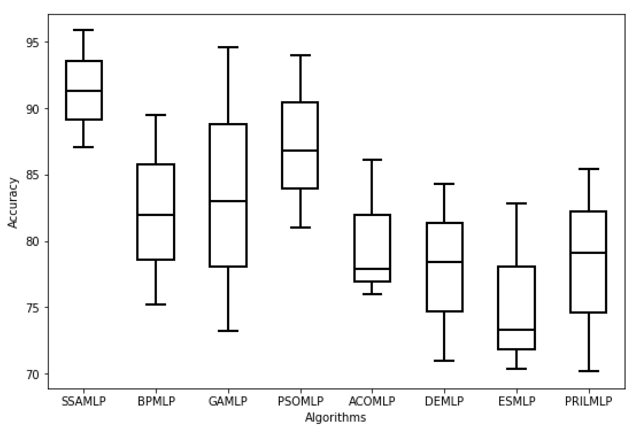
25	87.02	75.19	73.19	81.02	76.00	70.96	70.34	70.18

and Figure 5 show the accuracy results of the proposed SSAMLP model versus other algorithms that are integrated into the MLP algorithm.

As can be seen in Table 5, the best MLP structure is achieved when the number of hidden nodes is four and the number of layers is one. The results show that in the first three experiments, the accuracy of all hybrid models increases dramatically by decreasing the number of hidden nodes in the MLP’s structures. This can be explained because reducing the complexity of computations enhances the performance of DF prediction. The accuracy results increase until a specified limit, which is when the number of layers is one and the number of hidden nodes is four. This structure represents the best MLP structure for all algorithms in which the best DF prediction accuracy is achieved. After that, the accuracy started to decrease linearly by decreasing the number of nodes in the middle layer. The reason is that decreasing the number of nodes in the middle layer makes the model become simple, and the computations are not sufficient to produce an efficient model. Hence, it is not recommended to decrease the number of hidden nodes to less than four or increase it to more than four.

Choosing a medium number of computational nodes in the middle layer can produce the best classification model and achieve the best DF prediction performance. In the remaining experiments, the number of layers in the MLP structure does not benefit the prediction performance. Conversely, increasing the number of layers inversely affects the classification performance. This can increase the complexity of the classification model and cause a major machine learning problem, which is overfitting. This problem occurs because complex models that are unable to produce a general prediction pattern in the learning phase are generated. The produced model is complex and passes by a large number of learning instances. This reflects badly on the testing phase and causes degradation in the prediction performance. Figure 6 shows the convergence curves of the proposed SSAMLP versus other algorithms. The Y-axes is the error rate in terms of MSE. The X-axis is the number of iterations. It can be seen that SSAMLP achieved the best convergence curves, as it obtains the least error rates in the final iterations.

Overall, the experiments confirm that MLP can be applied as a reliable prediction model for DF. Furthermore, it can be revealed that the number of features is sufficient to investigate the DF and identify the application programs that have affected the file system. The best accuracy achieved is 95.84%, which is somehow high. This indicates that there is about a 4.16 error rate. Although there is no recommended error rate threshold commonly reported for the DF models, it can be explained that this small error rate comes from the application programs that access the same files in the file system. This makes the extracted features of the application programs overlap for several files.

6. Conclusions and Future Works

Recently, cybercrime has increased significantly and tremendously. This made the need for DF urgent. The target of this paper is to propose the SSA in training MLPs. The few parameters, fast convergence, and strong ability to avoid local minima motivated our attempts to use SSA to train MLPs. This is a minimization problem in which the main objective is to select the optimal structure of MLP (best connection weight and bias parameters) to achieve the minimum MSE. The purpose is to apply the optimal MLP in determining the growing evidence by checking the historical acts on the file system to identify how the application programs affected these files.

The used dataset in the experiments has been collected based on applying for five different application programs and checking the footprint on the system files that are the results of system actions and log entries. There are four scenarios for applying the application programs to the system files. These represent simple, medium, and complex scenarios to access the file system. The dataset is used to train the hybrid MLP-SSA model and determine the best structure of MLP that produces the minimum MSE. The results of the experiments show that the proposed SSAMLP outperformed others compared with hybrid meta-heuristic algorithms in terms of accuracy, error rate, and convergence scale. Furthermore, SSAMLP proved its suitability to be used as a reliable model to investigate DF, with an accuracy of 95.84% when the number of middle layers is one and the number of hidden nodes is four.

To verify the proposed method, a set of meta-heuristic algorithms were applied to the same dataset, and their results were compared with the SSAMLP. The comparison results show the out-performance of the SSAMLP in the majority of cases.

For future works, it is worthy to train other types of MLPs using the SSA. The applications of the multiobjective SSA to train MLP in the context of DF are recommended as well.