Constructing Domain Ontology for Alzheimer Disease Using Deep Learning Based Approach

Abstract

Facts can be exchanged in multiple fields with the help of disease-specific ontologies. A range of diverse values can be produced by mining ontological approaches for demonstrating disease mechanisms. Alzheimer’s disease (AD) is an incurable neurological brain illness. An early diagnosis of AD can be helpful for better treatment and the prevention of brain tissue destruction. Researchers have used machine learning techniques to predict the early detection of AD. However, Alzheimer’s disorders are still underexplored in the knowledge domain. In the biomedical field, the illustration of terminologies and notions is essential. Multiple methods are adopted to represent these notions, but ontologies are the most frequent and accurate. Ontology construction is a complex and time-consuming process. The designed ontology relies on Disease Ontology (DO), which is considered the benchmark in medical practice. Ontology reasoning mechanisms can be adopted for AD identification. In this paper, a deep convolutional neural network-based approach is proposed to diagnose Alzheimer’s disease, using an AD dataset acquired from Kaggle. Machine learning-based approaches (logistic regression, gradient boosting, XGB, SGD, MLP, SVM, KNN, random forest) are also used for a fair comparison. The simulation results are generated using three strategies (default parameters, 10-cross validation, and grid search), and MLP provides superior results on a default parameter strategy with an accuracy of 92.12%. Furthermore, the deep learning-based approach convolutional neural network (CNN) achieved an accuracy of 94.61%. The experimental results indicate that the construction of ontology, with the help of deep learning knowledge, can produce better results where the robustness and scalability can be enhanced. In comparisons to other methods, the CNN results are excellent and encouraging.

1. Introduction

Ontology Learning (OL) is an effective procedure that automatically extracts a manuscript’s knowledge and represents it in a machine-understandable form. However, the manual process of constructing ontologies is time-consuming, extremely laborious, and costly. There are two approaches used to extract knowledge from text, the linguistics-based approach, and the ML-based approach [1]. Ontology construction helps to translate raw data into a meaningful representation of knowledge.

Multiple approaches exist to efficiently retrieve data using multidimensional theory. Semantic and thematic graph generation processes are used to extract useful knowledge. Additionally, data mining techniques are used to present knowledge and to demonstrate the accuracy of information retrieval [2].

In the medical field of ontology, many different ontological diseases have been addressed over time. However, there has been limited work carried out on brain ontology diseases. Neuroimaging is an advanced technology that has been used in the study of several human brain diseases, such as Alzheimer’s, autism spectrum disorder (ASD) and schizophrenia. Unfortunately, little research is available on how to improve the study of brain diseases by incorporating ontological approaches. Recently, the design and use of neuron-based analytical tools has increased [3,4]. Many machine learning (ML) classifiers have been used in the diagnosis of brain diseases. Particle swarm optimization (PSO) is perceived as the most probable population-based stochastic algorithm and, as such, it is used to tackle global optimization problems [5,6,7,8,9,10,11]; BA is also widely used in such fields to find out the optimal answers to problems [12,13]. Alzheimer’s disease (AD) is recognised as a neuron-degenerative disease. Alzheimer’s disease consists of neurofibrillary tangles and senile plaque [14].

Previously, case bases were used for representation, but, currently, the most potent method for representation is ontology. The ontology construction process is not easy and requires a significant time and effort to build. Several ontology systems have been developed that allow for users to get useful information. Ontology construction in the biomedical field for brain disorders, especially when considering AD, is challenging [15].

The primary goal of our work is presented as follows:

• To investigate the performance of ML-based and DL-based approaches applied on the AD dataset.
• To evaluate the results using three strategies (default parameters, 10-cross validation, grid search).
• To use traditional machine learning and deep learning models for comparative analysis.
• To show that experimental simulation results depict that the deep learning model has attained state-of-the-art performance in different performance metrics.

The rest of the paper is structured as follows: Section 2 discusses the literature review. In Section 3, materials and methods are elaborated. Experimental results are presented in Section 4. In Section 5, a comparative analysis of the results is presented. The conclusion and future work are given in Section 6.

2. Literature Review

Shubuta proposed an ontology construction method for the detection of Alzheimer’s disease. The scope and domain coverage of ADO was evaluated by answering the questions with 72.31% accuracy [16].

A new domain-specific ontology construction technique for Alzheimer’s disease was proposed by Ash tosh Malhotra et al., who presented methodology formulated according to the life cycle of ontology building. Portege OWL was used as the ontology construction web language composition. N-gram analysis and noun phrase chunking are two stages that deal with an n-list of Alzheimer’s disease phrases and assign a frequency to each term [17].

According to [18], a common kind of dementia is Alzheimer’s disease, including its moderate cognitive impairment (MCI) phase. A novel machine learning-based approach is used to identify the following four biomarkers: FDG-PET, structural magnetic resonance imaging (sMRI), cerebrospinal fluid (CSF) 20 protein levels, and the Apo lipoprotein-E (APOE) genotype. The baseline dataset for the Alzheimer’s disease neuroimaging 21 initiative (ADNI) was used in this investigation.

This study [19] aims to predict the proper conversion of mitigated cognitive impairment (MCI) into magnetic resonance imaging (MRI) by using convolutional neural networks (CNN). The Alzheimer’s disease neuroimaging initiative (ADNI) is used for validation. The CNN prediction performance achieved 79.9% accuracy.

A statistical method is used for feature selection to produce a histogram for the early detection of AD. AD/HC, MCI/HC and sMCI/pMCI, achieved an accuracy of 84.17%, 70.38%, and 61.05%, respectively [20].

Detection and classification of Alzheimer’s disease is a challenging task using MRI data for elderly persons. Additionally, automatic Alzheimer disease detection is carried out with the Open Access Series of Imaging Studies (OASIS) dataset, using the ensemble deep neural networks and achieving higher accuracy [21].

In [22], due to the incurable nature of AD, different treatments are used to improve patients’ and their families’ quality of life. AD is still not sufficiently explainable to allow for successful universal therapies. The case-based reasoning (CBR) research paradigm supports the medical research method for finding treatments. The CBR is also used to establish whether or not a neuroleptic drug is given.

J. Islam detects Alzheimer’s disease by using several statistics and machine learning methods. For diagnosing AD, a neural network-based approach finds distinct phases of Alzheimer’s disease, and it is able to achieve higher performance for early-stage diagnosis using a brain MRI with the OAIS dataset [23].

The authors [24] suggested an intelligent and precise, two-dimensional deep convolutional neural network (2D-DCNN) for unbalanced MRI datasets. Experimental results provide an accuracy of 86.2%. For a fair comparison, state-of-the-art techniques are used, while 2D-DCNN show significant improvements.

The authors [25] utilized the convolutional neural network to detect AD. They have effectively categorized functional MRI data of people living with Alzheimer’s using the CNN and LeNet-5 architecture. The model achieved an accuracy of 86.85%. A comparative overview for all mentioned factors is presented in

Table 1. Comparison of Existing Relevant Approaches.

Sr. No.	Primary Study	Methodology	Dataset	Classifier	Accuracy
1	[26]	5ML-papline	ADNI	Random Forest	86.84%
2	[27]	PET (FDG-PET)	OASIS	Random Forest	84.17%
3	[19]	Free-feature based	ADNI	CNN	79.9%
4	[28]	Hybrid	ADNI		75.1%
5	[29]	ALZFUZZYONT	Alzheimer	Rule Bases	76.1%
6	[17]	Alzheimer disease ontology	Alzheimer	CBOW, skip-gram	72.91%
7	[16]	Foundry principles	Alzheimer	Formal Rules
8	[18]	FDG-PET	ADNI	ML Classifier	72.31%
9	[24]	Hybrid approaches	Alzheimer	(2D-DCNN)	86.2%.
10	[25]	LeNet-5 architecture	Alzheimer	CNN	86.85%.

.

3. Materials and Methods

There are many classification algorithms available in machine learning and deep learning. The major classification algorithms are listed below:

3.1. Support Vector Machine (SVM)

SVM is an ML classifier that we have applied in our study. This model is a three-dimensional spreading response record in interplanetary, at an expanse as open as conceivably possible, classifying the points based on their place in space. Calculations are carried out using the same formula as the knowledge information was spread on this new data. It is helpful in scenarios wherever the mechanism has to function in multi-class space, as it classifies numbers without giving chance checks, which are then costly to calculate using 10-Cross Validation.

3.2. Stochastic Gradient Descent (SGD)

Stochastic gradient descent is a simple, efficient, and advanced model for linear modelling which supports certain loss functions and penalties in categorizing a large amount of input data. Its simplicity, efficiency, and ability to process a large amount of data make it a useful model. As it is a fast and advanced model, it requires different hyperparameters for training, and is sensitive for scaling the features. Stochastic gradient descent is a very popular and common algorithm used in various machine learning algorithms, most importantly forming the basis of neural networks. In this article, I have tried my best to explain it in detailed yet simple terms. Gradient, in plain terms, means the slope or slant of a surface [30]. Gradient descent, then, means descending a slope to reach the lowest point on that surface.

3.3. Gradient Boosting Classifier (GBC)

Gradient boosting is a regression and classification machine learning approach that produces a prediction model in the form of an ensemble of weak prediction models. This method constructs a model step by step, and then establishes it by enabling the optimization of any differentiable loss function. Gradient boosting combines several relatively weak prediction models to create a more powerful prediction model [31].

3.4. K Nearest Neighbor (KNN)

The K-NN algorithm is a data mining method that is used for classification and regression problems. This algorithm assigns an object to a class according to the majority classes of the object’s neighbors. The value of K is set to a positive integer that describes the number of neighbors to be considered for the query. It is used for sentimental analysis because of its accurate results, and is a probabilistic classifier that works based on the Bayes’ theorem to judge the category of a particular instance. It applies the conditional probability model taking X = (X₁, X₂ … X_n) T inputs, and then allocates probability to the instances as given. It is a common model, and is stress-free to train if input data is erratically shifting and in huge amounts [32].

3.5. Decision Tree

A decision tree is a model that is used to organise a dataset comprised of fixed rules based on particular qualities and their pertinent modules. It is an easy-to-understand and control classifier, which does not need intricate information or excessive training and test data. It is very beneficial for both quantitative and qualitative data. However, it is subtle and can generate inconsistent or difficult to exercise results if a small inaccuracy happens in the training data, dependent on small values of entered variants. Different examples discussed previously indicate that decision trees are simple and easily understandable by anyone even outside the profession, including consumers. Decision trees are also useful in situations where the comparative variables belong to different types of data or have different rounding off/scaling, which is not possible with other logarithmic operations because decision trees are a structured representation, and rounding off does not affect them. Decision trees also do not get disturbed if there is some missing data during the programming process. Partitioning is based on the proportionality between split ranges, and is not absolute in the decision trees, so outliers do not get disturbed. These features allow this model to save time, which is another advantage of the decision tree [26].

3.6. Random Forest (RF)

The random forest is a model that uses the same principles as the decision tree. It generates different decision trees from the same input data on a random selection basis, and then matches all those subtrees to improve output accuracy. It offers superior accuracy because of its use of averages, as well as due to the fact that it has over-fitting controls, as compared to the decision tree model. Being an advanced model, it requires special knowledge for training and operation purposes. Classification is an important component of machine learning. Data science facilitates a family of algorithms, such as linear regression, naïve Bayes’, SVM, and the decision tree. As the name indicates, the random forest comprises of many individual decision trees that act as a whole. In the random forest, a class prediction is displayed on every tree. The model’s calculations are based on the class with the highest votes [33].

3.7. Multi-Layer Perceptron (MLP)

A feed-forward artificial neural network, called a multi-layer perceptron (MLP), creates a set of outputs from a collection of inputs. An MLP is distinguished by many layers of input nodes coupled as a directed graph between the input and output layers, implying that the signal route via the nodes is one-way only. Aside from the input nodes, each node has a nonlinear activation function. MLP uses backpropagation to train the network. MLP is a technique for deep learning.

3.8. XGB

Extreme gradient boosting (XGBoost) is a distributed gradient boosting toolkit that has been tuned for performance, adaptability, and mobility. It uses the gradient boosting framework to construct machine learning algorithms. It uses parallel tree boosting to handle a wide range of data science issues quickly and accurately. XGBoost is a machine learning method that has lately dominated Kaggle’s challenges for structured or tabular data [30].

3.9. Convolutional Neural Network (CNN)

Most of the time, a deep neural network is applied to analyze the images dataset. It is possible to study data images in one-dimensional and two-dimensional formats. To perceive the photographs as a human would is an ambiguous task for the machine, but it is actually a very easy one, because the computer vision is supported by the aid of a deep neural network. The working of this algorithm initiates when images are taken in the form of input. After the input, it assigns the weightage of the specific area of the images in the learnable context known as biases, and weightage to form the easy and quick difference between them. The pre-processing procedure is easy and reliable and requires less time when carried out within ConvNEt, compared to the various other classification algorithms.

CNN depends on the hidden layer/coat in the system model. Because of the convolutional coat, it is called a convolutional neural model. This coat supplies the particular convolutional operations needed to perceive the data. In the CNN model, input with the given weights of the groups with elevating the multi-linear operation is taken by a convolutional neural network, similar to other neural networks operating during the model. Between the 2D weighted array and input data array, there is a multiplication operation invoked, and it is recognised as a filter or kernel. The goal of developing the multiplication method is to input data in two and three dimensions. The dot product (x, y) category includes kernels and filters. The multiplication operation is performed element-by-element between the patch input filter size and the filter in dot product, resulting in a result that is always in the solitary form after the summer process.

In the case of a single output, the operation is completed and deliberated as the scalar product. Regardless of whether either of the patch input filter sizes is multiplied on the data, one criterion should always be remembered: the filter should be less than the input data obtained. The goal is to enable that filter to execute multiplication operations on the input array numerous times at different positions, in order to re-number the input. The filter is automatically applied to all overlapping areas, or the square input filter sizes data from all dimensions [14].

The same filter that applies to the image is commendable and valuable throughout with the help of the systematically and automatic application. If someone perceives or counts the particular field of the image data input in the existence of the various features in the images mentioned, the filter is solely applicable to the specific area, with particular and separated parts of the input data of the images that are needed to be retrieved. Although it can work and function well with one-dimensional or three-dimensional data, the convolutional neural network (CNN) is largely intended to function with two-dimensional data. The name of this network originated because of the middle layer that functions’ convolution, and, for this reason, it is named a convolutional layer. As with any other neural network, CNN also performs linear multiplication for the two-dimensional inputs, numerous arrays of input data, and 2D weights, known as kernels or filters.

Filter attributes are small in size as compared to the overall input data, and the result is the dot product of multiplication. Dot product in a component/quality wise multiplication between the kernel and kernels sized input set is summed up to produce a binary. In some cases, this kind of function is also known as ‘scalar product’. It is a recognized practice to utilize the small size of in screens rather than the entered value, because it offers the option of the similar screen to various overlying areas of the input data in altered dimensions. Application of the same filter on various areas of the image is very beneficial, as it permits the recognition of a particular features in the image, for which the filter design is intended. It is known as conversion invariance, and it allows for the recognition of the existence or lack a function alternate to the position of the feature [14].

4. Methodology

In our proposed methodology, as mentioned in Figure 1, the dataset is acquired from the repository UCI. In a pre-processing step, fMRI images are used. To balance the data, an up-sampling data augmentation approach is used. In the feature engineering step, feature extraction and selection are performed using machine learning approaches (random forest, extreme gradient boosting, multilayer perceptron (MLP), gradient boosting, support vector machine, stochastic gradient descent, logistic regression, and decision tree). These feature vectors are presented to the eight different machine learning classifiers for the detection of AD. Three different validation strategies (default parameter, 10-cross fold and grid search) are used for the fair results comparison. Machine learning-based approaches are used for manual feature selection, which is a time-consuming and unreliable method. For automatic feature selection, a deep learning-based convolutional neural network model is used for the early detection of AD.

A CNN is a DL method developed recently that has attracted considerable attention. In general, a CNN is a multi-layered network. A CNN consists of a series of convolution (C) and subsampling (S) layers. Each layer is composed of multiple 2D planes, with each serving as a feature map; the network also includes some fully connected (FC) hidden layers. There is only one input layer in a CNN. This input layer receives two-dimensional objects directly, and the process of feature extraction to samples is performed by the convolution and sampling layers. Multiple fully connected hidden layers are mostly used for realizing specific tasks.

Certain hyperparameters are used during the training stage to improve the CNN model results. This is because the performance of any deep learning model is affected by its hyper-parameter tuning. After using a batch size of 50, as well as a number of epoch of 50 and a learning rate of 0.0001, it produced superior outcomes for CNN models.

The third and final phase is the multi-classification of Alzheimer’s disease. The proposed approach uses ML and DL techniques to classify non-demented and demented Alzheimer’s patients’ data (very mild, mild, moderate). The data distribution is comprised of the dataset divided into train, test, and validation data. Accuracy can be increased by adjusting the model parameters. Accuracy is evaluated in three perspectives, default parameters, 10-cross validation, and grid search CV.

Model evaluation was carried out using various machine learning methods for data classification. On testing data, the model predicts the probability of an AD patient or non-AD patient. In the end, the performance evaluation gave insights into the knowledge of the model by depicting its performance and construction of AD ontology.

To check the performance of machine learning and deep learning models, we compared them with state-of-the-art approaches from the literature to determine which provided better results. The primary purpose is to facilitate ontology developers in the ontology construction process. The basic purpose of this work is the construction of ontology in a unique manner.

Identification of the ontology module refers to the study that decides the aspect that will confirm the system of the construction of the ontology.

The ontology construction module is compulsory in order to join all concepts into a single group. Similar terms and concepts are grouped into smaller clusters. A cluster consists of all domain-related terms and knowledge, and generates a fully defined list of classes, termed the identification module in ontology construction. The same classes or concepts in the same module are grouped under a single name in order to facilitate their use in the future. The names of the modules clarify the related terms, classes, and relations between individuals. Researchers use predefined and particular knowledge to solve the problems.

4.1. Dataset

The Open Access Series of Imaging Studies (OASIS) is a collection of magnetic resonance imaging data sets that are publicly accessible for research and study. The data set consisted of 416 individuals ranging in age from 18 to 96 years old. One hundred of the participants, all over the age of 60, were identified as having very mild to moderate Alzheimer’s disease. All of the subjects are right-handed, and both genders are included [28].

4.2. Dataset Collection

This research used data from Kaggle, a free open-access platform. The study relied on the Alzheimer’s Dataset, which included MRI scans. The following four classes were present in the dataset: very mildly demented, mildly mentally retarded, moderately retarded, and non-demented. Figure 2 shows the amount of data and image samples used in the experiment.

4.3. Nine Images with Labels

Figure 3 shows a grid of 9 images selected for training the data set. This nine-image grid is labeled as Mild Demented, Moderate Demented, Non Demented, and Very Mild Demented in the prediction of Alzheimer’s disease.

4.4. Data Pre-Processing

Data pre-processing refers to studies in which the most important aspect is to increase the quality of the data. This stage counts as a critical step for data analysis concerning improving the quality of data. During pre-processing, SES and MMSE have true values that belong to null values. This null value is removed by utilizing respective columns. Full anomalies/null values are removed from the dataset and transformed into meaningful forms. The purpose of cleaning up the data is to overcome the outlier problem that occurs during the construction of AD diagnosis. Attributes included for this comparative work are detailed in

Table 2. Measures Included in the Data Set.

Serial No.	Variable Name	Variable Description
1	Group	the state of the patient (Demented, Non-Demented, Converted)
2	ID	Identification of patient
3	M/F	Gender (Male, Female)
4	Hand	Left-Handed, Right-Handed
5	Age	Age during scanning of brain image
6	EDUC	Years of education
7	SES	Socioeconomic Status of the patient
8	CDR	Clinical Dementia Rating
9	eTIV	Estimated/experimental Total Intracranial Volume
10	nWBV	Normalize Whole Brain Volume
11	MRI ID	Patient MRI Number
12	ASF	Atlas Scaling Factor
13	MRI Delay	Delay
14	Visit	Number of visits to the doctor

.

The rate of AD disease in the demented and non-demented groups varies with age. In the demented group, the rate for females is lower during the eighties age-period, while the male rate is higher. Similarly, in non-demented groups, the females’ rate is higher than the male. Alzheimer’s disease is more common in males than in women, according to the bird-eye view available in Figure 4.

This histogram graph explains the AD rate in terms of the age perspective in Figure 5. The AD rate mostly starts from age 60, and continually increases to age 90. The earlier stage starts at the age of 60–65 years, which counts as very mild. At the age of 65–70 years, mild AD is encountered, and at the age of 70–75 severe AD is encountered. Demented patients had a higher percentage of AD at between 70 and 80 years and, thus, have a lower survival rate than non-demented patients.

4.5. Evaluation Metrics

Several assessment criteria are used to evaluate the performance of the various classifiers. These criteria help to determine whether a model is good for classification or prediction. By using these assessment metrics, the best algorithm can also be identified. In this research study, the following assessment criteria were used: accuracy, precision, recall, and F1-score. All of the equations used for computation are detailed in

Table 3. Evaluation Metrics.

Metric	Equation
Accuracy	(TP+ TN + FP + FN)/(TP + TN)
Precision	TP/(TP + FP)
Recall	TP/(TP + FN)
F1-Score	2 (Precision × Recall)/(Precision + Recall)

Where TP, TN, FP, FN stands for True Positive, True Negative, False Positive and False Negative.

. For simulation, a GPU Enabled machine is used and detailed specs are listed in

Table 4. GPU Supported Computing Machine Specifications used for Experiments.

Sr.	Item	Specifications
1	Model-Series	Lenovo Legion 7
2	Processor	Intel® Core™ i7-10750H Processor (2.60 GHz, up to 5.00 GHz with Turbo Boost, 6 Cores, 12 Threads, 12 MB Cache)
3	Generation	10th Generation
4	RAM	32 GB DDR4 2933 MHz
5	Screen Size/Resolution	15.6″, FHD (1920 × 1080) Anti-glare, 144 Hz
8	Graphic Card	NVIDIA® GeForce RTX™ 2070 Max-Q 8 GB
9	Hard Disk	1 TB

.

5. Classification Results

The different machine learning and deep learning models were tested on the OASIS dataset for different performance metrics precision, recall, accuracy, and f1-score.

5.1. Accuracy Comparison of ML Models

In this section, ML-based approaches’ accuracy is calculated with three different strategies default parameters, 10-cross validation and Grid Search. Among these three strategies, default parameters provide the best result.

Figure 6 explains the comparison of different ML models with respect to their accuracy based on default parameters. The MLP beats the other ML classifiers with 92.12%, while in Figure 7, the comparison of different ML models is explained with respect to their accuracy based on 10-Cross Validation. The MLP beats the other ML classifiers with 89.69%. Additionally, a comparison of different ML models with respect to their accuracy based on Grid Search is presented in Figure 8, where the Random Forest beats the other ML classifiers with 89.84%.

In

Table 5. Comparison of ML with State of the Art.

Parameter	Previous Work	Previous Work	Previous Work	Previous Work	Proposed Methodology
MLP (ACC)	75.1%	79.9%	84.17%	86.84%	92.12%
Author	[28]	[19]	[27]	[26]	Proposed
Attributes	9	15	10	11	9
Database	ADNI	MeSH	J-ADNI	OASIS	OASIS

, state-of-the-art algorithms are compared with ML approaches used in this study, where MLP gives superior results over previous approaches.

5.2. Model Assessment Results Using Machine Learning

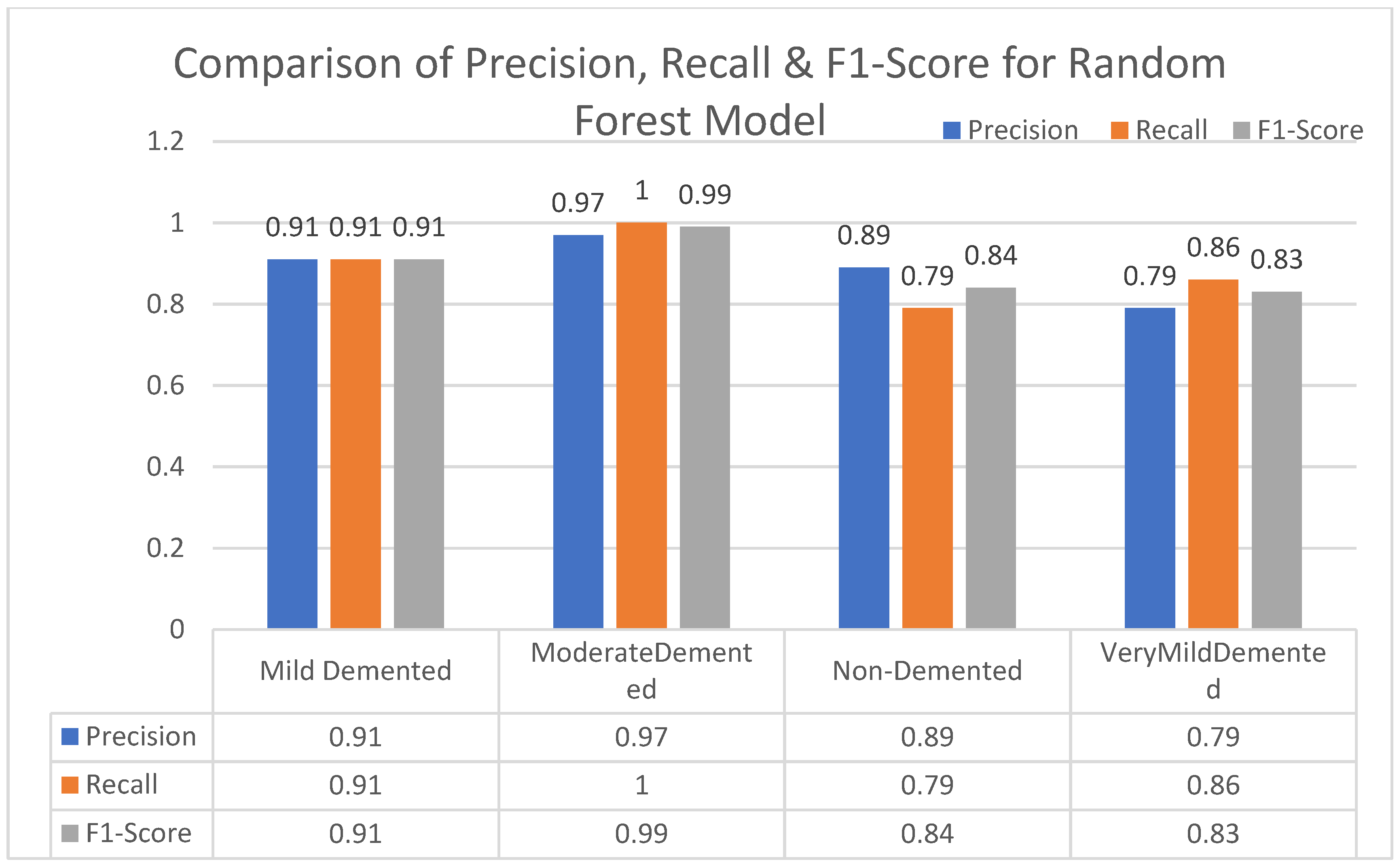
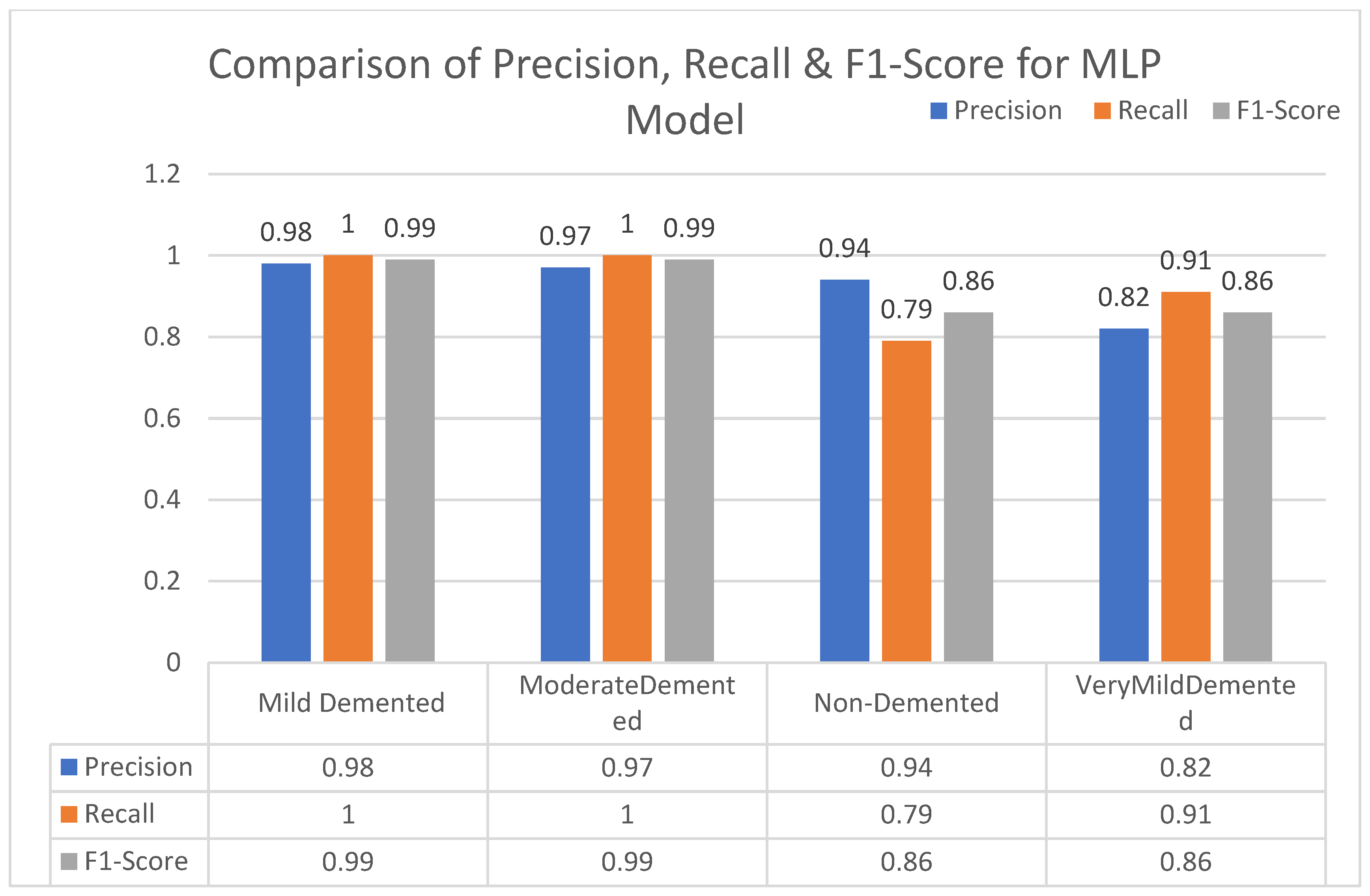
In this section, we carried out an evaluation of metrics parameters precision, recall, and the f1-score of multiclass (very mild, mild, moderated and non-demented) Alzheimer disease of each ML algorithm. Multiclass of Alzheimer disease is discussed.

Moderate demented shows higher values of precision, recall, and F1-Score as compared to the other stages in all machine learning models. Mild demented shows higher values of precision, recall and f1-score as compared to the other stages as presented in Figure 9, Figure 10, Figure 11, Figure 12, Figure 13, Figure 14 and Figure 15.

5.3. Deep Learning Model Development

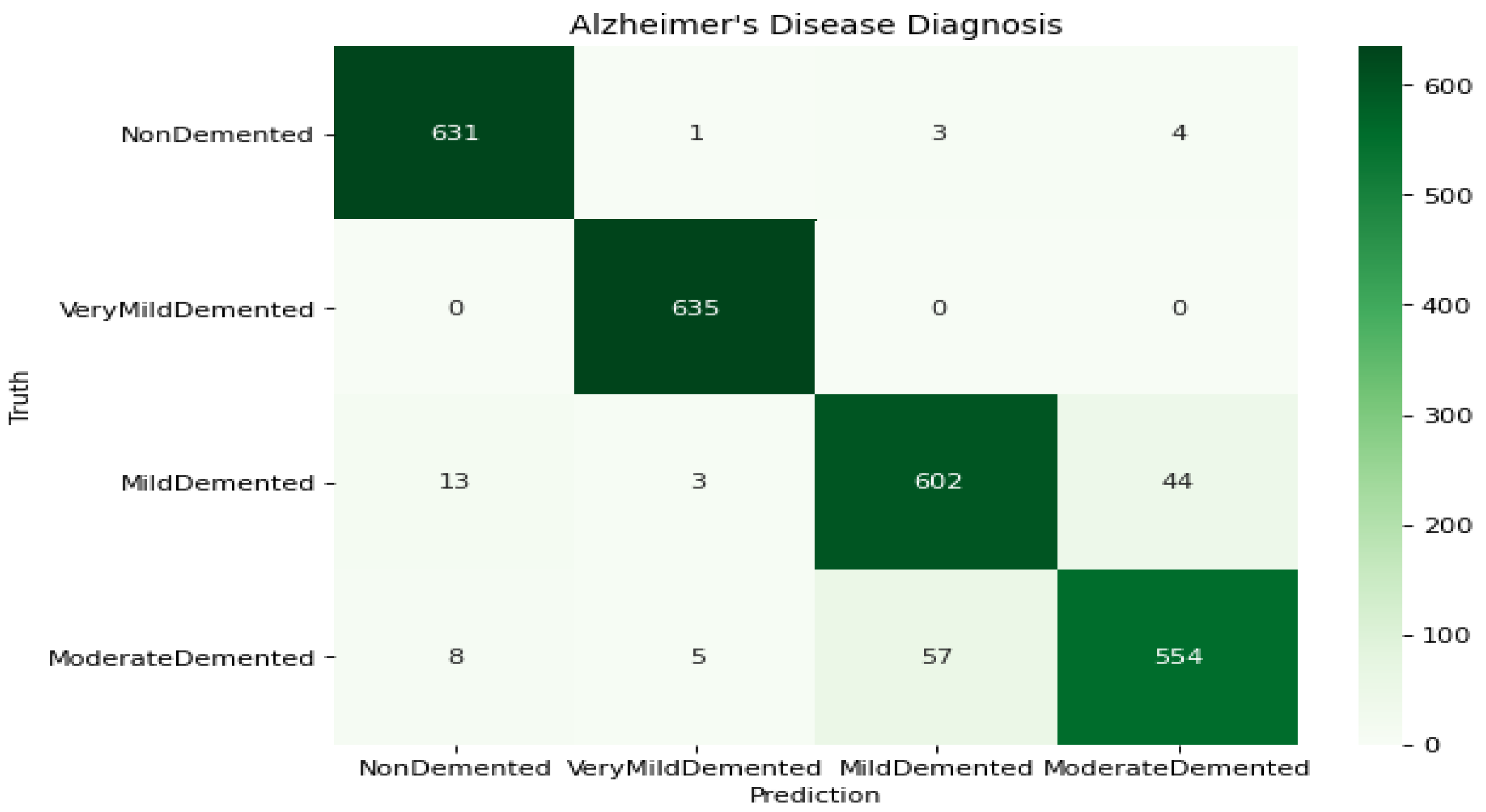
This section applies the CNN model to predict the Alzheimer stages (mild demented, moderate demented, non-demented and very mild demented). The CNN model is checked based on performance metrices, such as accuracy, recall, F1-Score, and precision. These measurement parameters are used to evaluate to CNN models.

In Figure 16, the above graph shows metrics trends during training of the dataset. The trends are positive from low to high and achieve the DL accuracy is 94.61%. DL gained high accuracy during testing. The confusion matrix in Figure 17 was produced when the network was tested with test data after training.

5.4. Classification Report of Tested Data

Figure 18 explains the precision, recall, F1-score, of four labels classes. Very Mild Demented precision is high 0.99, non-demented class precision is 0.97.

5.5. Comparative Discussion

In this section,

Table 6. Comparative Analysis of Machine Learning and Deep Learning Classifiers’ Accuracy.

Comparison	Algorithm	Accuracy
Machine Learning	MLP	92.12%
Deep Learning	CNN	94.61%

shows a comparative analysis of ML and DL with respect to accuracy. By using the default parameters strategy, MLP provides the best results. Similarly, a DL-based approach CNN gives 94.61% on the given AD dataset. By comparing ML and DL results, it is clear that the DL-based approach is superior to the ML algorithms.

In

Table 7. Comparison of DL with State of Art.

Model	Previous Work	Previous Work	Previous Work	Previous Work	Proposed Methodology
CNN (ACC)	78%	79.93%	89.76%	90%	94.63%
Author	[23]	[34]	[35]	[36]	Proposed

, CNN is compared with the state-of-the-art approaches taken from the literature; the results depict that the CNN acquired a higher accuracy of 94.63%.

5.6. Ontology of AD Implementing Using Protégé

The ontology construction is performed using Protégé version 4.0.4. Protégé provides a facility for representation context, as well as in a graph visualization format and modification. It facilitates graph representation according to user requirement. Ontology web language (OWL) is used to construct the ontology. In Protégé, OWL is considered as a Java-based application. It is used to represent the knowledge base and domain base system that can plug in the architecture, as shown in Figure 19 and Figure 20.

6. Conclusions and Future Direction

AD is a kind of dementia which affects elderly adults. It can cause a variety of health issues, including memory loss. For the early detection of disease, computer aided solutions are necessary. This paper applies ML and DL-based approaches (logistic regression, gradient boosting, SGD, MLP, SVM, KNN, and random forest) to the AD dataset OASIS. The experiment results are generated using three strategies (default parameters, 10-cross validation, grid search). The ML-based approach MLP using default parameter provides an accuracy 92.12%, while the DL-based approach CNN gives the highest accuracy at 94.61%. For a fair comparison, machine learning and deep learning-based approaches are compared with examples from the literature. The results indicate that CNN is accurate with regards to performance. The ontology designed completely relies on disease ontology (DO), which is considered the benchmark in the medical field. The results shows that DL-based approaches are very beneficial for early-stage AD diagnosis. The main feature of ontology construction is to provide the reasoning behind the development of ontology. Protégé software was used to carry out the mapping of Alzheimer’s ontology in which access will be possible through a semantic web.

In the future, we plan to evaluate the proposed model for different AD datasets and other brain disease diagnoses. A real-time model can be developed that will help doctors diagnose Alzheimer patients.