Machine Learning Techniques for the Prediction of the Magnetic and Electric Field of Electrostatic Discharges


Abstract
:1. Introduction
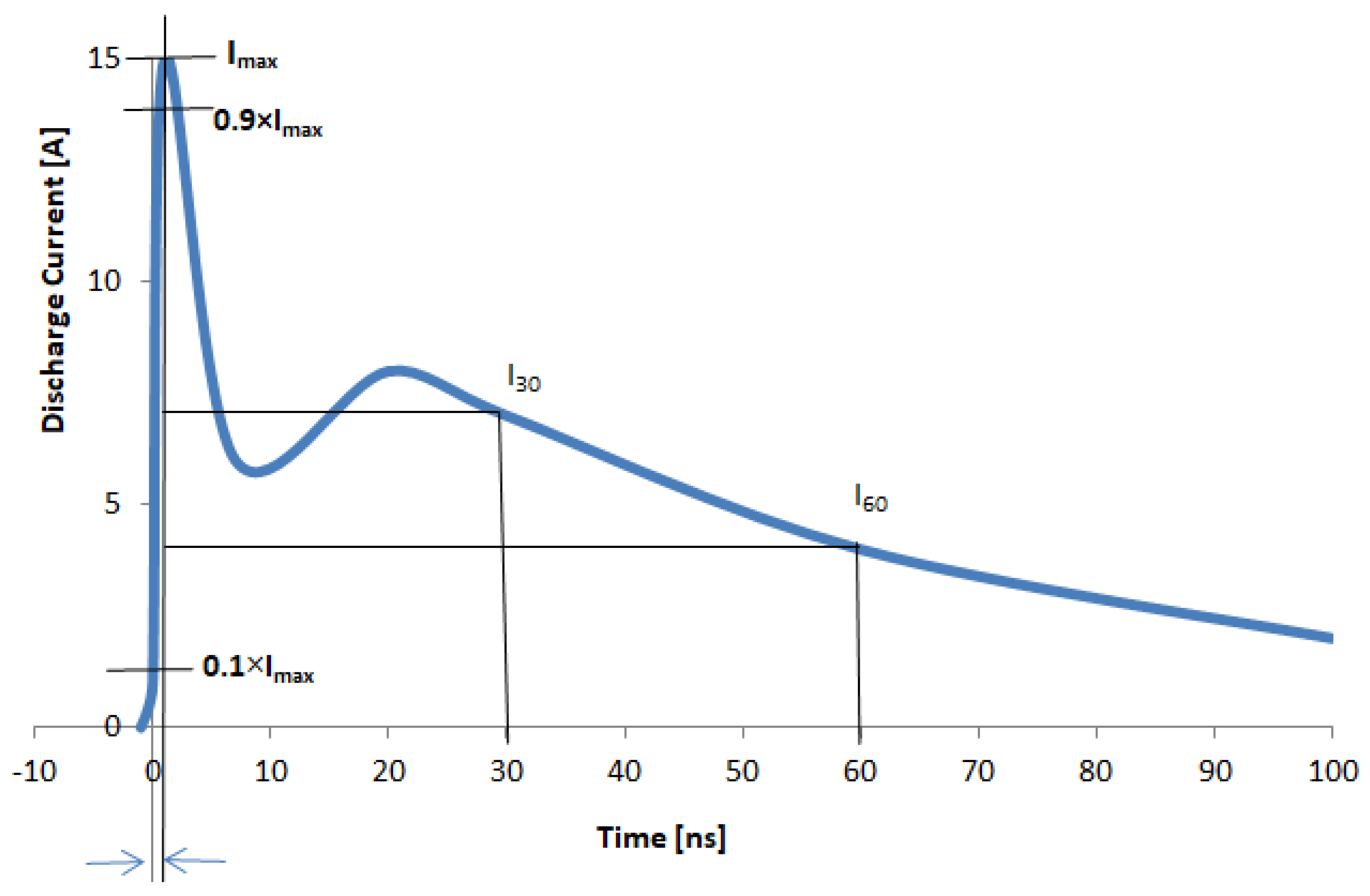
2. The IEC 61000-4-2
3. Current and EM Field Measurements
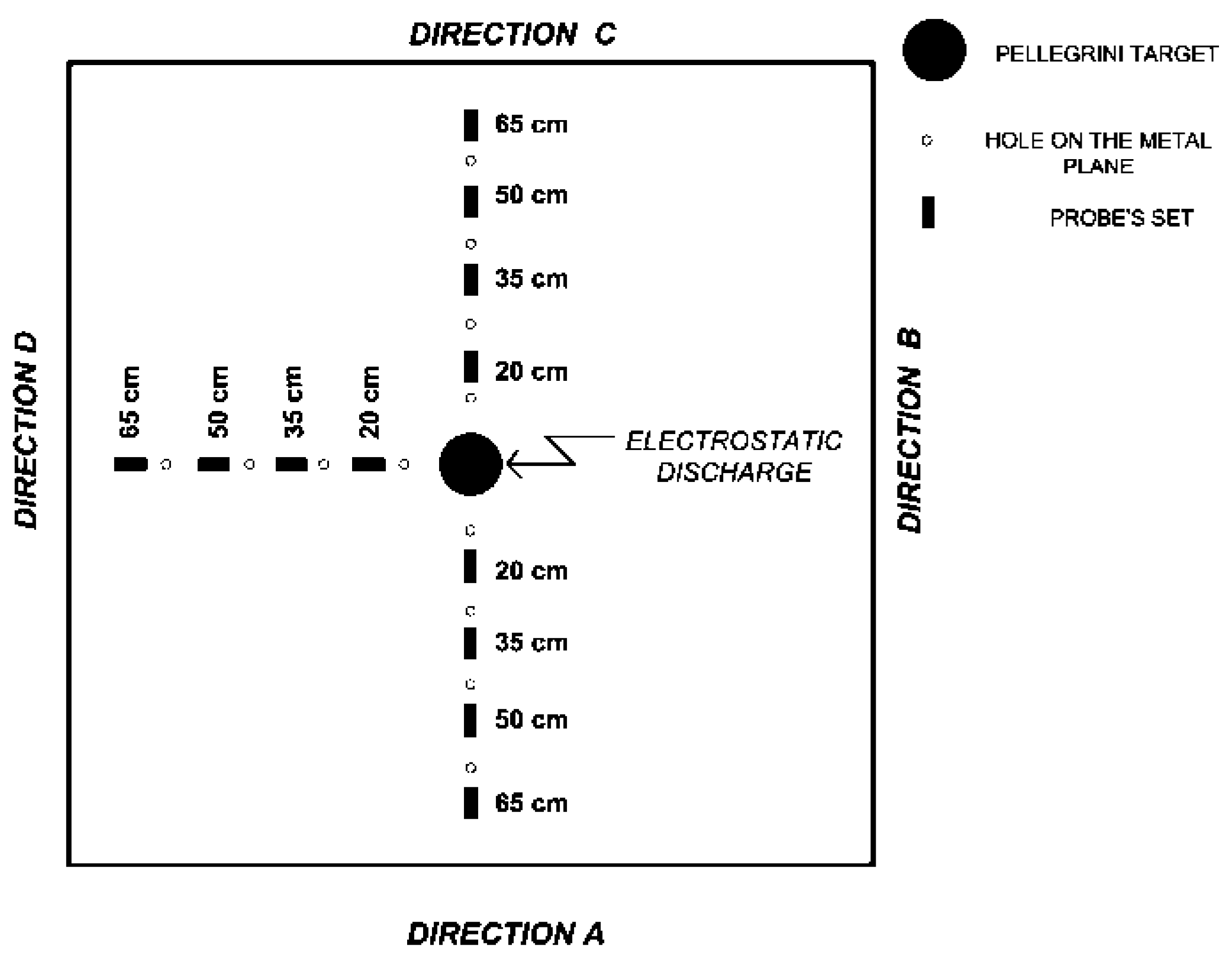
3.1. Laboratory Setup
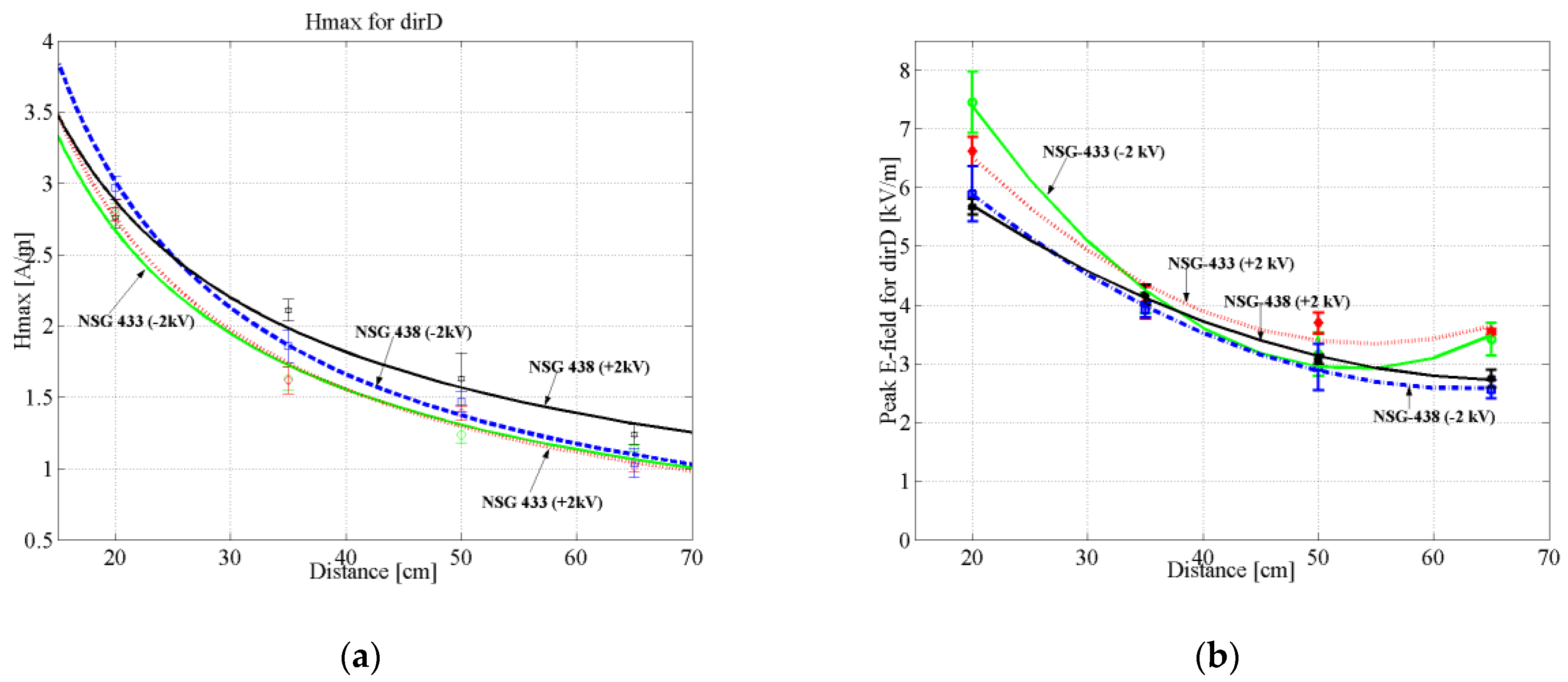
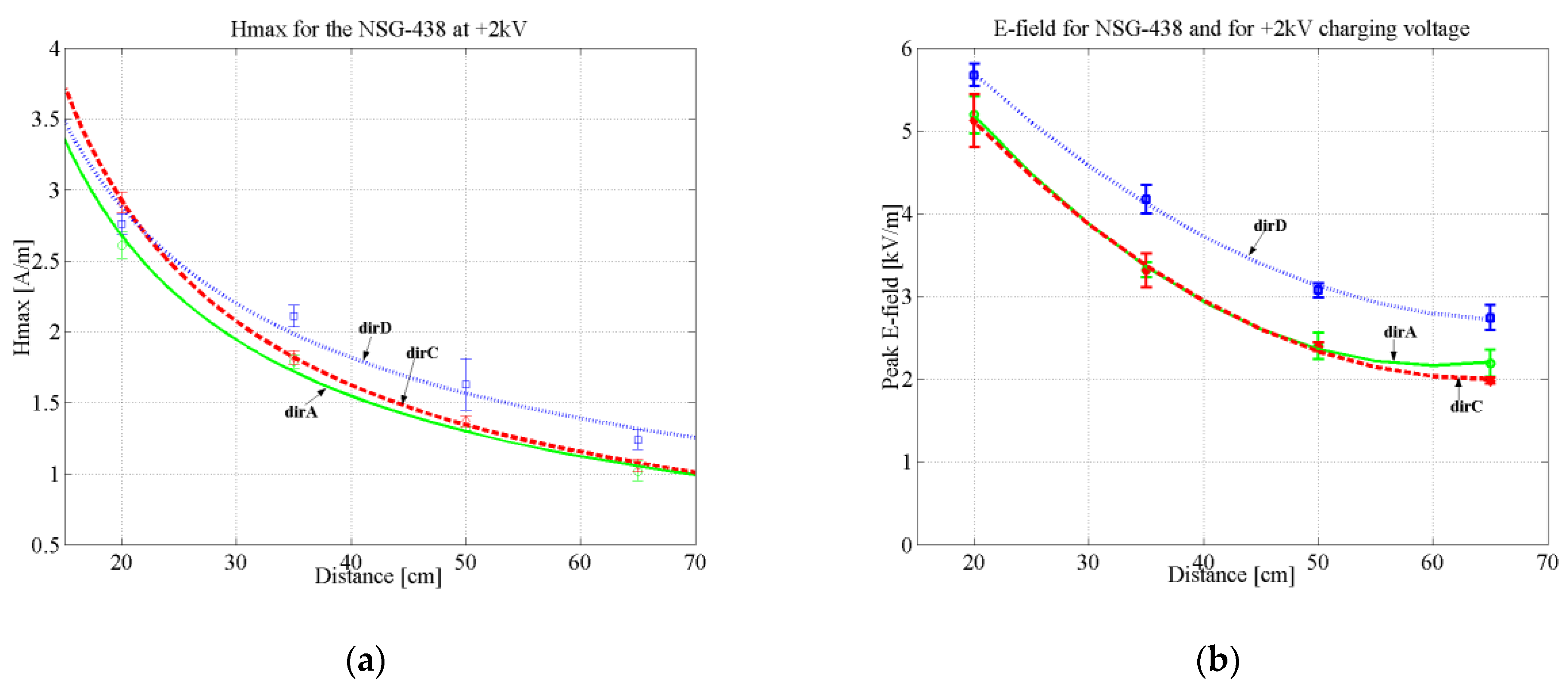
3.2. Laboratory Results
4. Machine Learning
4.1. Learning Classifiers—Bayes Rule
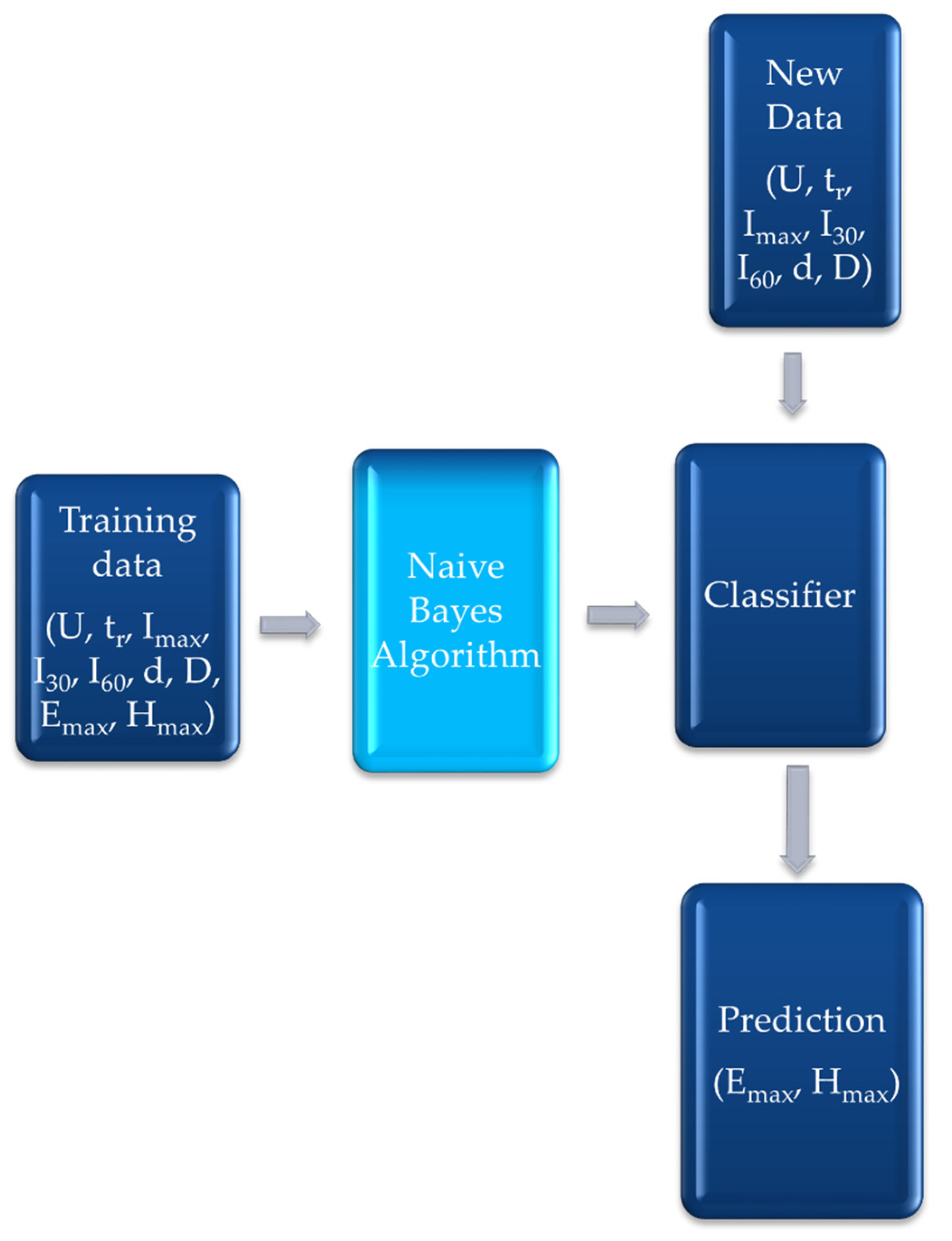
4.2. Naïve Bayes Algorithm
4.2.1. Conditional Independence
4.2.2. Derivation of NBA
4.2.3. Logistic Regression
5. Design and Implementation of the Developed NBA
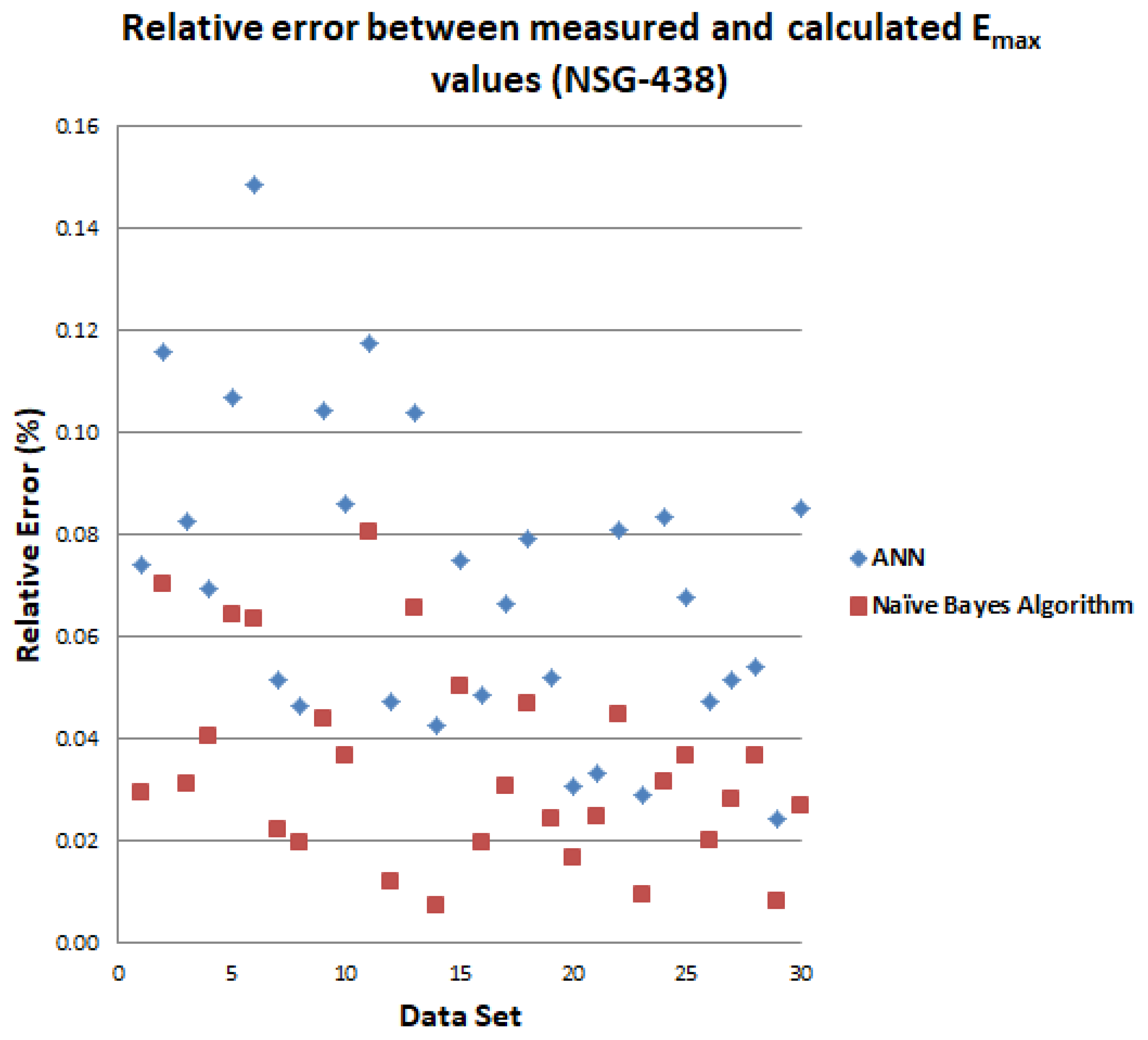
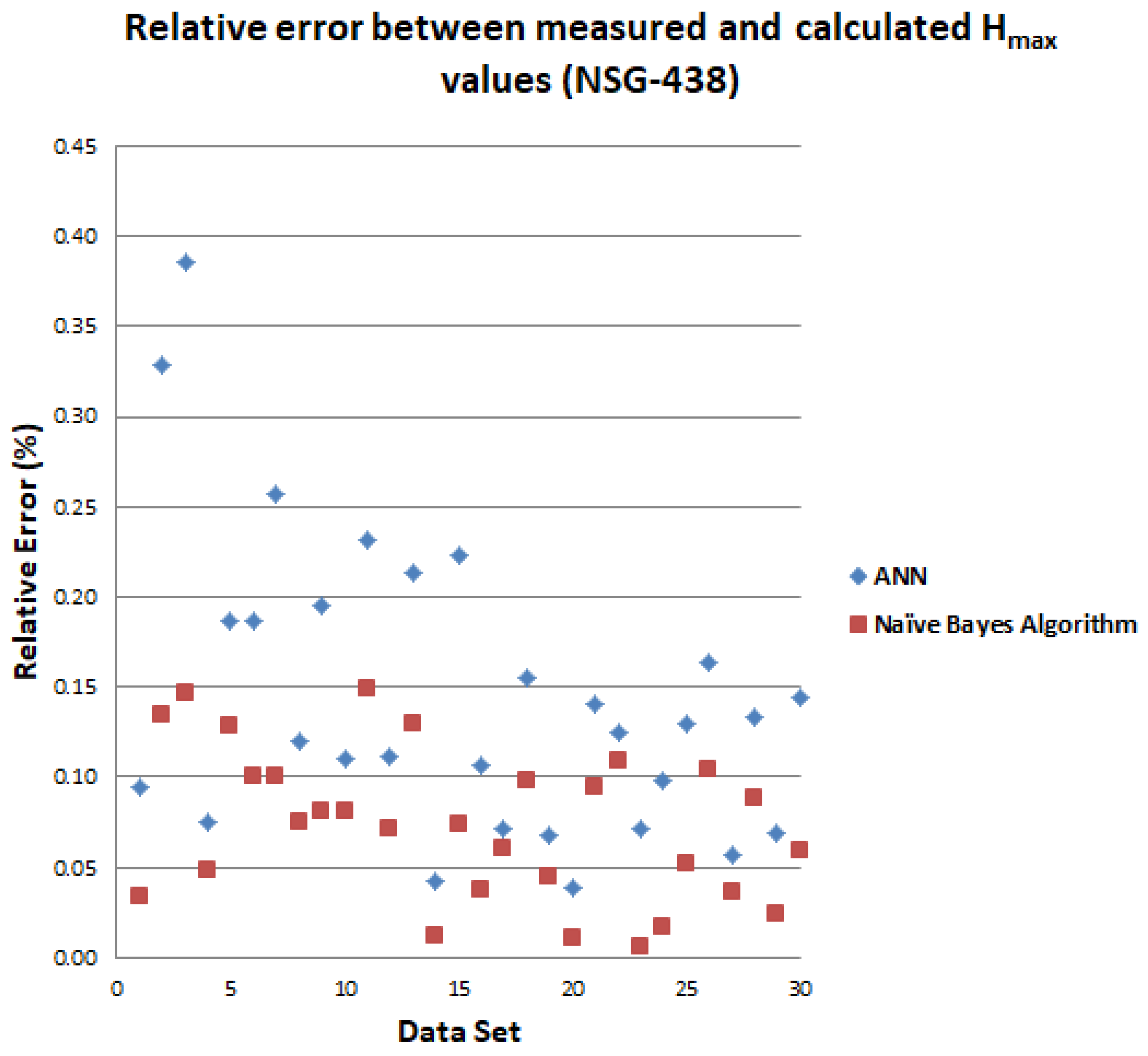
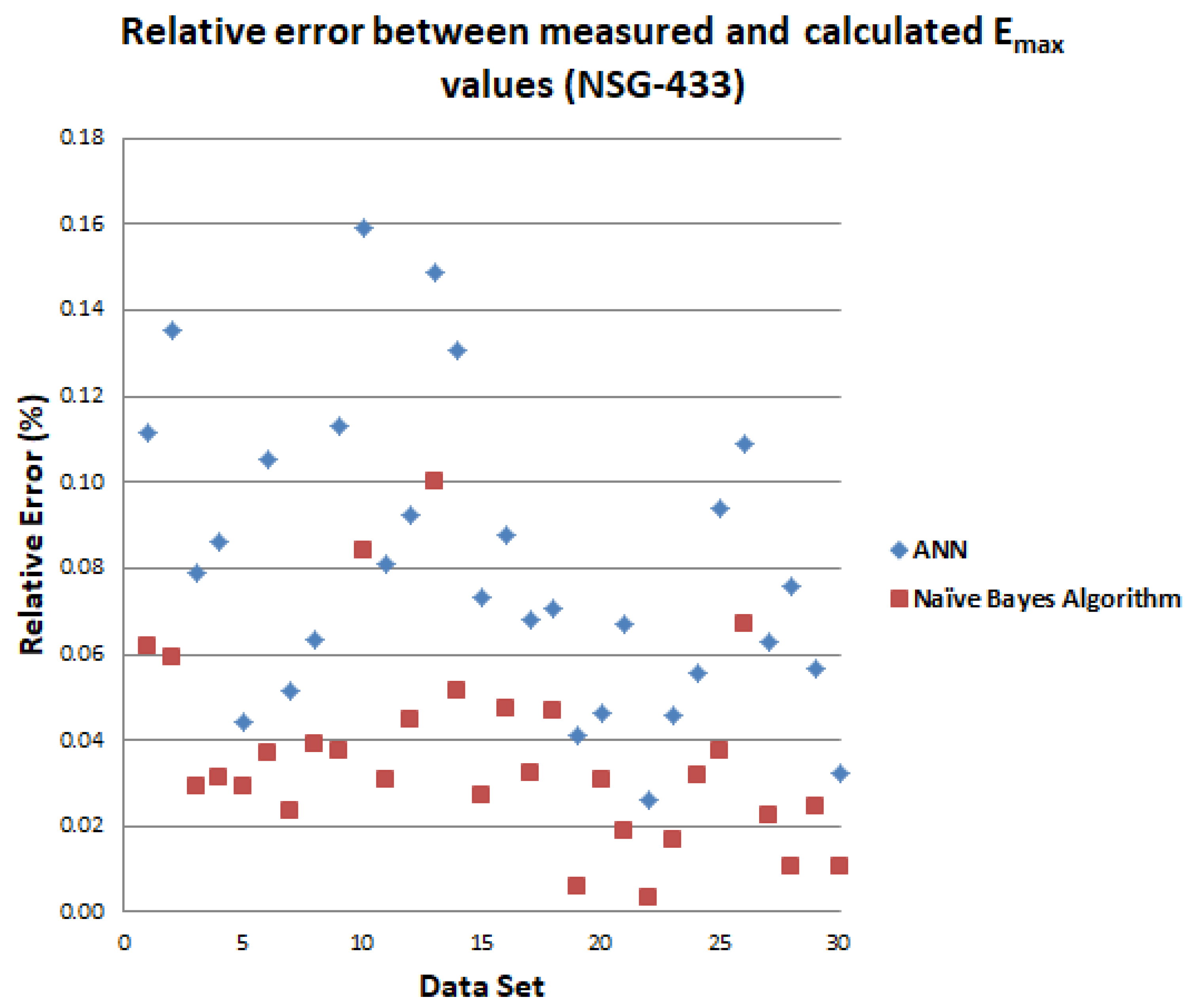
6. Results-Discussion
7. Conclusions
Author Contributions
Funding
Data Availability Statement
Acknowledgments
Conflicts of Interest
References
- Wang, A. Practical ESD Protection Design, 1st ed.; Wiley-IEEE Press: Piscataway, NJ, USA, 2021. [Google Scholar]
- Bafleur, M.; Caignet, F.; Nolhier, N. ESD Protection Methodologies: From Component to System, 1st ed.; ISTE Press—Elsevier: Singapore, 2017. [Google Scholar]
- Luo, G.X.; Huang, K.; Zhou, J.C.; Zhang, W.; Pommerenke, D.; Holliman, J. Design of an Artificial Dummy for Human Metal Model ESD. IEEE Trans. Electromagn. Compat. 2021, 63, 319–323. [Google Scholar] [CrossRef]
- Joint HBM Working Group ESD Association and JEDEC Solid State Technology Association. User Guide of ANSI/ESDA/JEDEC JS-001 Human Body Model Testing of Integrated Circuits. Available online: https://www.jedec.org/sites/default/files/JTR001-01-12%20Final.pdf (accessed on 1 June 2022).
- Llovera-Segovia, P.; Domínguez-Lagunilla, M.; Fuster-Roig, V.; Quijano-López, A. Electrostatics comfort in buildings and offices: Some experiences and basic rules. J. Electrost. 2022, 115, 103650. [Google Scholar] [CrossRef]
- Holdstock, P. A review of electrostatic standards. J. Electrost. 2022, 115, 103652. [Google Scholar] [CrossRef]
- Yousaf, J.; Lee, H.; Nah, W. System level ESD analysis—A comprehensive review on ESD generator modeling. J. Electr. Eng. Technol. 2018, 13, 2017–2032. [Google Scholar] [CrossRef]
- Pommerenke, D. EMC fundamentals—ESD. In Proceedings of the IEEE International Symposium on Electromagnetic Compatibility & Signal/Power Integrity (EMCSI), Gaithersburg, MD, USA, 4–12 August 2017. [Google Scholar] [CrossRef]
- Yousaf, J.; Shin, J.; Lee, H.; Nah, W.; Youn, J.; Lee, D.; Hwank, C. Efficient Circuit and an EM Model of an Electrostatic Discharge Generator. IEEE Trans. Electromagn. Compat. 2018, 60, 1078–1086. [Google Scholar] [CrossRef]
- Oganezova, I.; Pommerenke, D.; Zhou, J.; Ghosh, K.; Hosseinbeig, A.; Lee, J.; Tsitskishvili, N.; Jobava, T.; Sukhiashvili, Z.; Jobava, R. Human body impedance modelling for ESD simulations. In Proceedings of the IEEE International Symposium on Electromagnetic Compatibility Signal/Power Integrity, Washington, DC, USA, 7–11 August 2017. [Google Scholar] [CrossRef]
- IEC 61000-4-2. Electromagnetic Compatibility (EMC)—Part 4-2: Electrostatic Discharge Immunity Test, ed. 2.0. 2008. Available online: https://webstore.iec.ch/publication/4189 (accessed on 22 March 2021).
- Ishida, T.; Tozawa, Y.; Fujiwara, O. Effect of Approach Speed on Spark Length determining Air Discharge Current from ESD Generator in Environment with Different Temperature and Humidity. In Proceedings of the IEEE International Joint EMC/SI/PI and EMC Europe Symposium, Raleigh, NC, USA, 26 July–13 August 2021. [Google Scholar] [CrossRef]
- Ishida, T.; Fujiwara, O. Further Effects of Test Voltages, Relative Humidity and Temperature on Air Discharge Currents from Electrostatic Discharge Generator. In Proceedings of the Sapporo and Asia-Pacific International Symposium on Electromagnetic Compatibility, Sapporo, Japan, 3–7 June 2019. [Google Scholar] [CrossRef]
- Ishida, T.; Fujiwara, O. Specific Dependence on Absolute Humidity and Saturation Deficit of Air Discharge Currents from Electrostatic Discharge Generator with Different Approach Speeds. In Proceedings of the IEEE International Symposium on Electromagnetic Compatibility, Signal & Power Integrity (EMC + SIPI), New Orleans, LA, USA, 22–26 July 2019. [Google Scholar] [CrossRef]
- Xiu, Y.; Sagan, S.; Battini, A.; Ma, X.; Raginsky, M.; Rosenbaum, E. Stochastic modeling of air electrostatic discharge parameters. In Proceedings of the IEEE International Reliability Physics Symposium (IRPS), Burlingame, CA, USA, 11–15 March 2018. [Google Scholar] [CrossRef]
- Wilson, P.F.; Ma, M.T. Field radiated by electrostatic discharges. IEEE Trans. Electromagn. Compat. 1991, 33, 10–18. [Google Scholar] [CrossRef]
- Pommerenke, D. ESD: Transient fields, arc simulation and rise time limit. J. Electrost. 1995, 36, 31–54. [Google Scholar] [CrossRef]
- Kim, K.C.; Lee, K.S.; Lee, D.I. Estimation of ESD current waveshapes by radiated electromagnetic fields. IEICE Trans. Commun. 2000, 83, 608–612. [Google Scholar]
- Ishigami, S.; Gokita, R.; Nishiyama, Y.; Yokoshima, I. Measurements of fast transient fields in the vicinity of short gap discharges. IEICE Trans. Commun. 1995, 78, 199–206. [Google Scholar]
- Frei, S.; Pommerenke, D. A transient field measurement system to analyze the severity and occurrence rate of electrostatic discharge (ESD). J. Electrost. 1998, 44, 191–203. [Google Scholar] [CrossRef]
- Leuchtmann, P.; Sroka, J. Transient field simulation of electrostatic discharge (ESD) in the calibration setup (ace. IEC 61000-4-2). In Proceedings of the International Symposium on EMC, Washington, DC, USA, 21–25 August 2000. [Google Scholar]
- Leuchtmann, P.; Sroka, J. Enhanced field simulations and measurements of the ESD calibration setup. In Proceedings of the International Symposium on EMC, Montreal, QC, Canada, 13–17 August 2001. [Google Scholar]
- Becanovic, N.; Mousavi, S.M.; Fellner, G.; Pommerenke, D. A Portable Test Platform for Capturing ESD Induced Fields. In Proceedings of the IEEE International Joint EMC/SI/PI and EMC Europe Symposium, Raleigh, NC, USA, 26 July–13 August 2021. [Google Scholar] [CrossRef]
- Li, D.Z.; Zhou, J.; Hosseinbeig, A.; Pommerenke, D. Transient electromagnetic co-simulation of electrostatic air discharge. In Proceedings of the 39th Electrical Overstress/Electrostatic Discharge Symposium (EOS/ESD), Tucson, AZ, USA, 10–14 September 2017. [Google Scholar] [CrossRef]
- Ishigami, S.; Kawamata, K.; Minegishi, S.; Fujiwara, O. Measurement of electric field waveform caused by micro gap ESD in a pair of spherical electrodes In Proceedings of the Asia-Pacific International Symposium on Electromagnetic Compatibility (APEMC), Seoul, Korea, 20–23 June 2017. [CrossRef]
- Kawamata, K.; Ishigami, S.; Minegishi, S.; Fujiwara, O. Distance characteristic of electric field waveform and field peak value caused by micro gap ESD in a pair of spherical electrodes. In Proceedings of the International Symposium on Electromagnetic Compatibility—EMC EUROPE, Angers, France, 4–7 September 2017. [Google Scholar] [CrossRef]
- Fotis, G.P.; Ekonomou, L.; Maris, T.I.; Liatsis, P. Development of an artificial neural network software tool for the assessment of the electromagnetic field radiating by electrostatic discharges. IEE Proc. Sci. Meas. Technol. 2007, 1, 261–269. [Google Scholar] [CrossRef]
- Fotis, G.P.; Ekonomou, L.; Maris, T.I.; Liatsis, P. Estimation of the electromagnetic field radiating by electrostatic discharges using artificial neural networks. Simul. Model. Pract. Theory 2007, 15, 1089–1102. [Google Scholar] [CrossRef]
- Vita, V.; Fotis, G.P.; Ekonomou, L. An Optimization Algorithm for the Calculation of the Electrostatic Discharge Current Equations’ Parameters. WSEAS Trans. Circuits Syst. 2016, 15, 224–228. [Google Scholar]
- Vita, V.; Fotis, G.P.; Ekonomou, L. Parameters’ optimisation methods for the electrostatic discharge current equation. Int. J. Energy 2017, 11, 1–6. [Google Scholar]
- Cestnik, B. Estimating probabilities: A crucial task in machine learning. In Proceedings of the 9th European Conference on Artificial Intelligence, Stockholm, Sweden, 6–10 August 1990. [Google Scholar]
- Clark, P.; Niblett, T. The CN2 induction algorithm. Mach. Learn. 1989, 3, 261–283. [Google Scholar] [CrossRef]
- Duda, R.; Hart, P. Pattern Classification and Scene Analysis, 1st ed.; Wiley: New York, NY, USA, 1973. [Google Scholar]
- Kasif, S.; Salzberg, S.; Waltz, D.; Rachlin, J.; Aha, D.W. A probabilistic framework for memory-based reasoning. Artif. Intell. 1998, 104, 297–312. [Google Scholar] [CrossRef]
- Langley, P.; Iba, W.; Thompson, K. An analysis of Bayesian classifiers. In Proceedings of the 10th National Conference on Artificial Intelligence, Menlo Park, CA, USA, 12–16 July 1992. [Google Scholar]
- Domingos, P.; Pazzani, M. On the optimality of the simple Bayesian classifier under zero-one loss. Mach. Learn. 1997, 29, 103–130. [Google Scholar] [CrossRef]
- Wang, K.; Pommerenke, D.; Chundru, R.; Doren, T.V.; Drewniak, J.L.; Shashindranath, A. Numerical modeling of electrostatic discharge generators. IEEE Trans. Electromagn. Compat. 2003, 45, 258–270. [Google Scholar] [CrossRef]
- Mitchel, T.M. Machine Learning, 1st ed.; McGraw-Hill: New York, NY, USA, 1997; pp. 154–199. [Google Scholar]
- Hu, J.; Niu, H.; Carrasco, J.; Lennox, B.; Arvin, F. Voronoi-Based Multi-Robot Autonomous Exploration in Unknown Environments via Deep Reinforcement Learning. IEEE Trans. Veh. Technol. 2020, 19, 14413–14423. [Google Scholar] [CrossRef]
- Chen, S.; Webb, I.G.; Liu, L.; Ma, L.X. A novel selective naïve Bayes algorithm. Knowl.-Based Syst. 2020, 192, 105361. [Google Scholar] [CrossRef]
- Zhang, H.; Jiang, L. Fine tuning attribute weighted naive Bayes. Neurocomputing 2022, 488, 402–411. [Google Scholar] [CrossRef]
- Omran, S.; El Houby, E.M.F. Prediction of electrical power disturbances using machine learning techniques. J. Ambient Intell. Humaniz. Comput. 2020, 11, 2987–3003. [Google Scholar] [CrossRef]
- Belik, I. A Comparative Analysis of the Neural Network and Naive Bayes Classifiers. 2018. Available online: https://papers.ssrn.com/sol3/papers.cfm?abstract_id=3371889#maincontent (accessed on 2 June 2022).
- Shi, Y.; Lu, X.; Niu, Y.; Li, Y. Efficient Jamming Identification in Wireless Communication: Using Small Sample Data Driven Naive Bayes Classifier. IEEE Wirel. Commun. Lett. 2021, 10, 1375–1379. [Google Scholar] [CrossRef]
- Raschka, S. Naïve Bayes and Text Classification I: Introduction and Theory. 2017. Available online: https://arxiv.org/abs/1410.5329 (accessed on 2 May 2022).


| Level | Charging Voltage (kV) | Imax (A) | Accepted Deviation | tr (ns) | Accepted Deviation | I30 (A) | Accepted Deviation | I60 (A) | Accepted Deviation |
|---|---|---|---|---|---|---|---|---|---|
| 1 | 2 | 7.5 | ±15% | 0.8 | ±25% | 4 | ±30% | 2 | ±30% |
| 2 | 4 | 15 | 8 | 4 | |||||
| 3 | 6 | 22.5 | 12 | 6 | |||||
| 4 | 8 | 30 | 16 | 8 |
| Input Variables | Output Variables |
|---|---|
| charging voltage (U) | maximum electric field value (Emax) |
| maximum discharge current (Imax) | maximum magnetic field value (Hmax) |
| current at 30 ns (I30) | |
| current at 60 ns (I60) | |
| rise time (tr) | |
| distance (d) | |
| direction (D) |
| Schaffner ESD Generator NSG-433 | |||||||||||||||||
|---|---|---|---|---|---|---|---|---|---|---|---|---|---|---|---|---|---|
| Varying Parameters | Measured | ANN | NBA | ||||||||||||||
| …No. | U (kV) | tr (ns) | Imax (A) | I30 (A) | I60 (A) | d (cm) | D | E (kV/m) | H (A/m) | E (kV/m) | R.E. (%) | H (A/m) | R.E. (%) | E (kV/m) | R.E. (%) | H (A/m) | R.E. (%) |
| 1 | +2 | 0.77 | 6.95 | 3.78 | 2.44 | 35 | A | 4.04 | 2.03 | 4.49 | 0.11 | 2.31 | 0.14 | 4.29 | 0.06 | 2.15 | 0.06 |
| 2 | +2 | 0.75 | 7.17 | 3.69 | 2.45 | 65 | A | 2.36 | 1.38 | 2.68 | 0.14 | 1.57 | 0.14 | 2.50 | 0.06 | 1.48 | 0.07 |
| 3 | +2 | 0.76 | 7.13 | 3.95 | 2.50 | 35 | C | 3.42 | 1.64 | 3.69 | 0.08 | 1.89 | 0.15 | 3.52 | 0.03 | 1.75 | 0.07 |
| 4 | +2 | 0.73 | 7.28 | 3.93 | 2.39 | 65 | C | 2.55 | 0.95 | 2.77 | 0.09 | 0.79 | 0.17 | 2.63 | 0.03 | 0.99 | 0.04 |
| 5 | +2 | 0.73 | 7.34 | 3.67 | 2.43 | 35 | D | 4.08 | 1.68 | 4.26 | 0.04 | 1.88 | 0.12 | 4.20 | 0.03 | 1.75 | 0.04 |
| 6 | +2 | 0.76 | 7.16 | 3.62 | −2.40 | 65 | D | 3.52 | 1.12 | 3.89 | 0.11 | 1.33 | 0.19 | 3.65 | 0.04 | 1.22 | 0.09 |
| 7 | −2 | 0.75 | −7.19 | −3.99 | −2.41 | 20 | A | −9.75 | −2.98 | −9.25 | 0.05 | −2.78 | 0.07 | −9.52 | 0.02 | −2.90 | 0.03 |
| 8 | −2 | 0.78 | −7.12 | −3.80 | −2.42 | 35 | A | −4.11 | −1.88 | −3.85 | 0.06 | −1.57 | 0.16 | −3.95 | 0.04 | −1.72 | 0.09 |
| 9 | −2 | 0.76 | −7.13 | −3.87 | −2.43 | 50 | A | −2.65 | −1.75 | −2.95 | 0.11 | −1.95 | 0.11 | −2.75 | 0.04 | −1.86 | 0.06 |
| 10 | −2 | 0.74 | −7.18 | −3.99 | −2.41 | 65 | A | −2.26 | −1.61 | −2.62 | 0.16 | −1.88 | 0.17 | −2.45 | 0.08 | −1.78 | 0.11 |
| 11 | −2 | 0.73 | −7.19 | −3.92 | −2.37 | 20 | C | −6.55 | −2.93 | −6.02 | 0.08 | −3.24 | 0.11 | −6.35 | 0.03 | −3.12 | 0.06 |
| 12 | −2 | 0.73 | −7.18 | −3.95 | −2.41 | 35 | C | −3.35 | −1.67 | −3.04 | 0.09 | −1.93 | 0.16 | −3.20 | 0.04 | −1.75 | 0.05 |
| 13 | −2 | 0.77 | −7.18 | −3.90 | −2.42 | 50 | C | −2.69 | −0.94 | −2.29 | 0.15 | −1.13 | 0.20 | −2.42 | 0.10 | −1.02 | 0.09 |
| 14 | −2 | 0.72 | −7.12 | −3.99 | −2.44 | 65 | C | −2.52 | −0.81 | −2.85 | 0.13 | −1.18 | 0.46 | −2.65 | 0.05 | −1.01 | 0.25 |
| 15 | +4 | 0.71 | 14.75 | 7.19 | 5.08 | 20 | A | 3.68 | 12.28 | 3.95 | 0.07 | 12.92 | 0.05 | 3.78 | 0.03 | 12.54 | 0.02 |
| 16 | +4 | 0.75 | 14.75 | 7.05 | 5.04 | 35 | A | 2.96 | 7.18 | 3.22 | 0.09 | 7.52 | 0.05 | 3.10 | 0.05 | 7.29 | 0.02 |
| 17 | +4 | 0.78 | 14.87 | 6.97 | 5.01 | 50 | A | 2.80 | 5.14 | 2.99 | 0.07 | 5.42 | 0.05 | 2.89 | 0.03 | 5.25 | 0.02 |
| 18 | +4 | 0.79 | 14.98 | 6.87 | 5.09 | 65 | A | 2.55 | 4.51 | 2.73 | 0.07 | 3.71 | 0.18 | 2.67 | 0.05 | 4.25 | 0.06 |
| 19 | +4 | 0.72 | 14.75 | 7.09 | 5.12 | 35 | C | 6.56 | 2.89 | 6.83 | 0.04 | 2.99 | 0.03 | 6.60 | 0.01 | 2.94 | 0.02 |
| 20 | +4 | 0.72 | 14.88 | 6.94 | 5.13 | 65 | C | 5.21 | 1.64 | 5.45 | 0.05 | 1.95 | 0.19 | 5.37 | 0.03 | 1.75 | 0.07 |
| 21 | +4 | 0.74 | 14.93 | 6.84 | 5.17 | 35 | D | 7.45 | 3.18 | 7.95 | 0.07 | 3.58 | 0.13 | 7.59 | 0.02 | 3.35 | 0.05 |
| 22 | +4 | 0.73 | 14.75 | 6.86 | 5.11 | 65 | D | 6.19 | 2.10 | 6.03 | 0.03 | 1.92 | 0.09 | 6.17 | 0.00 | 2.05 | 0.02 |
| 23 | −4 | 0.74 | −15.46 | −7.36 | −5.10 | 35 | A | −8.31 | −2.99 | −8.69 | 0.05 | −2.77 | 0.07 | −8.45 | 0.02 | −2.88 | 0.04 |
| 24 | −4 | 0.76 | −14.78 | −7.23 | −5.19 | 65 | A | −4.12 | −2.84 | −4.35 | 0.06 | −2.99 | 0.05 | −4.25 | 0.03 | −2.92 | 0.03 |
| 25 | −4 | 0.79 | −14.59 | −7.24 | −5.16 | 35 | C | −6.17 | −2.72 | −6.75 | 0.09 | −2.49 | 0.08 | −6.40 | 0.04 | −2.65 | 0.03 |
| 26 | −4 | 0.72 | −14.79 | −7.13 | −5.18 | 65 | C | −4.77 | −1.59 | −4.25 | 0.11 | −1.86 | 0.17 | −4.45 | 0.07 | −1.69 | 0.06 |
| 27 | −4 | 0.74 | −14.42 | −7.14 | −4.94 | 20 | D | −12.87 | −3.18 | −12.06 | 0.06 | −3.55 | 0.12 | −12.58 | 0.02 | −3.29 | 0.03 |
| 28 | −4 | 0.76 | −14.81 | −7.12 | −5.01 | 35 | D | −7.63 | −2.92 | −7.05 | 0.08 | −2.60 | 0.11 | −7.55 | 0.01 | −2.81 | 0.04 |
| 29 | −4 | 0.79 | −15.38 | −7.25 | −5.14 | 50 | D | −6.17 | −2.65 | −6.52 | 0.06 | −2.89 | 0.09 | −6.32 | 0.02 | −2.78 | 0.05 |
| 30 | −4 | 0.76 | −14.83 | −7.42 | −4.99 | 65 | D | −7.41 | −2.20 | −7.65 | 0.03 | −2.45 | 0.11 | −7.49 | 0.01 | −2.32 | 0.05 |
| Schaffner ESD Generator NSG-438 | |||||||||||||||||
|---|---|---|---|---|---|---|---|---|---|---|---|---|---|---|---|---|---|
| Varying Parameters | Measured | ANN | NBA | ||||||||||||||
| …No. | U (kV) | tr (ns) | Imax (A) | I30 (A) | I60 (A) | D (cm) | d (cm) | E (kV/m) | H (A/m) | E (kV/m) | R.E. (%) | H (A/m) | R.E. (%) | E (kV/m) | R.E. (%) | H (A/m) | R.E. (%) |
| 1 | +2 | 0.72 | 7.12 | 3.89 | 2.42 | 20 | A | 5.13 | 2.65 | 5.51 | 0.07 | 2.93 | 0.09 | 5.28 | 0.03 | 2.74 | 0.03 |
| 2 | +2 | 0.72 | 6.97 | 3.67 | 2.48 | 50 | A | 2.42 | 1.34 | 2.70 | 0.12 | 1.78 | 0.33 | 2.59 | 0.07 | 1.52 | 0.13 |
| 3 | +2 | 0.73 | 7.16 | 3.98 | 2.49 | 65 | A | 5.81 | 1.09 | 6.29 | 0.08 | 1.51 | 0.39 | 5.99 | 0.03 | 1.25 | 0.15 |
| 4 | +2 | 0.74 | 7.35 | 3.82 | 2.54 | 20 | C | 5.19 | 2.91 | 5.55 | 0.07 | 2.69 | 0.08 | 5.40 | 0.04 | 2.77 | 0.05 |
| 5 | +2 | 0.75 | 7.17 | 3.95 | 2.43 | 35 | C | 2.34 | 1.87 | 2.09 | 0.11 | 1.52 | 0.19 | 2.19 | 0.06 | 1.63 | 0.13 |
| 6 | +2 | 0.79 | 7.29 | 3.75 | 2.49 | 50 | C | 2.36 | 1.39 | 2.71 | 0.15 | 1.13 | 0.19 | 2.51 | 0.06 | 1.25 | 0.10 |
| 7 | +2 | 0.72 | 7.25 | 3.89 | 2.46 | 65 | C | 5.84 | 1.09 | 6.14 | 0.05 | 1.37 | 0.26 | 5.97 | 0.02 | 1.20 | 0.10 |
| 8 | +2 | 0.74 | 7.39 | 3.79 | 2.39 | 20 | D | 5.63 | 2.66 | 5.89 | 0.05 | 2.98 | 0.12 | 5.74 | 0.02 | 2.86 | 0.08 |
| 9 | +2 | 0.77 | 7.16 | 3.93 | 2.30 | 35 | D | 2.98 | 2.21 | 3.29 | 0.10 | 2.64 | 0.19 | 3.11 | 0.04 | 2.39 | 0.08 |
| 10 | +2 | 0.79 | 7.22 | 3.67 | 2.45 | 50 | D | 3.02 | 1.73 | 3.28 | 0.09 | 1.54 | 0.11 | 3.13 | 0.04 | 1.59 | 0.08 |
| 11 | +2 | 0.77 | 6.97 | 3.95 | 2.39 | 65 | D | 2.73 | 1.34 | 2.41 | 0.12 | 1.03 | 0.23 | 2.51 | 0.08 | 1.14 | 0.15 |
| 12 | −2 | 0.72 | −7.07 | 3.82 | −2.32 | 20 | A | −5.94 | −2.95 | −6.22 | 0.05 | −3.28 | 0.11 | −6.01 | 0.01 | −3.16 | 0.07 |
| 13 | −2 | 0.71 | −7.06 | −3.99 | −2.41 | 50 | A | −2.60 | −1.31 | −2.33 | 0.10 | −1.03 | 0.21 | −2.43 | 0.07 | −1.14 | 0.13 |
| 14 | −2 | 0.75 | −7.09 | −3.84 | −2.52 | 20 | C | −2.83 | −5.87 | −2.95 | 0.04 | −6.12 | 0.04 | −2.85 | 0.01 | −5.94 | 0.01 |
| 15 | −2 | 0.78 | −7.09 | −3.65 | −2.36 | 50 | C | −2.40 | −1.21 | −2.22 | 0.07 | −1.48 | 0.22 | −2.28 | 0.05 | −1.30 | 0.07 |
| 16 | −2 | 0.74 | −7.19 | −4.12 | −2.44 | 20 | D | −4.13 | −2.91 | −4.33 | 0.05 | −3.22 | 0.11 | −4.21 | 0.02 | −3.02 | 0.04 |
| 17 | −2 | 0.72 | −7.12 | −3.93 | −2.24 | 35 | D | −3.93 | −1.82 | −3.67 | 0.07 | −1.69 | 0.07 | −3.81 | 0.03 | −1.71 | 0.06 |
| 18 | −2 | 0.72 | −7.29 | −3.98 | −2.32 | 50 | D | −3.42 | −1.42 | −3.15 | 0.08 | −1.20 | 0.15 | −3.26 | 0.05 | −1.28 | 0.10 |
| 19 | +4 | 0.72 | 14.69 | 6.98 | 5.03 | 20 | A | 11.61 | 3.39 | 12.21 | 0.05 | 3.62 | 0.07 | 11.89 | 0.02 | 3.54 | 0.04 |
| 20 | +4 | 0.73 | 14.72 | 6.89 | 5.04 | 35 | A | 7.22 | 2.88 | 7.44 | 0.03 | 2.99 | 0.04 | 7.34 | 0.02 | 2.85 | 0.01 |
| 21 | +4 | 0.78 | 14.79 | 6.72 | 5.06 | 50 | A | 4.83 | 2.34 | 4.99 | 0.03 | 2.01 | 0.14 | 4.95 | 0.02 | 2.12 | 0.09 |
| 22 | +4 | 0.74 | 14.59 | 6.58 | 4.54 | 65 | A | 3.58 | 1.92 | 3.87 | 0.08 | 1.68 | 0.13 | 3.74 | 0.04 | 1.71 | 0.11 |
| 23 | +4 | 0.72 | 14.67 | 6.84 | 4.09 | 20 | C | 9.69 | 3.47 | 9.97 | 0.03 | 3.72 | 0.07 | 9.78 | 0.01 | 3.49 | 0.01 |
| 24 | +4 | 0.78 | 14.72 | 7.18 | 4.65 | 50 | C | 4.79 | 2.45 | 5.19 | 0.08 | 2.69 | 0.10 | 4.94 | 0.03 | 2.49 | 0.02 |
| 25 | +4 | 0.75 | 14.89 | 6.39 | 4.66 | 20 | D | 10.63 | 3.24 | 11.35 | 0.07 | 3.66 | 0.13 | 11.02 | 0.04 | 3.41 | 0.05 |
| 26 | +4 | 0.73 | 14.70 | 6.81 | 4.78 | 50 | D | 5.49 | 2.69 | 5.75 | 0.05 | 2.25 | 0.16 | 5.60 | 0.02 | 2.41 | 0.10 |
| 27 | −4 | 0.76 | −14.89 | −7.32 | −4.81 | 20 | A | −12.39 | −3.36 | −11.75 | 0.05 | −3.55 | 0.06 | −12.04 | 0.03 | −3.48 | 0.04 |
| 28 | −4 | 0.77 | −14.63 | −7.31 | −4.66 | 50 | A | −5.19 | −2.26 | −4.91 | 0.05 | −2.56 | 0.13 | −5 | 0.04 | −2.46 | 0.09 |
| 29 | −4 | 0.74 | −14.79 | −7.21 | −4.05 | 20 | C | −12.27 | −3.33 | −12.57 | 0.02 | −3.56 | 0.07 | −12.37 | 0.01 | −3.41 | 0.02 |
| 30 | −4 | 0.78 | −14.92 | −7.29 | −5.01 | 50 | C | −4.47 | −2.36 | −4.09 | 0.09 | −2.02 | 0.14 | −4.35 | 0.03 | −2.22 | 0.06 |
Publisher’s Note: MDPI stays neutral with regard to jurisdictional claims in published maps and institutional affiliations. |
© 2022 by the authors. Licensee MDPI, Basel, Switzerland. This article is an open access article distributed under the terms and conditions of the Creative Commons Attribution (CC BY) license (https://creativecommons.org/licenses/by/4.0/).
Share and Cite
Fotis, G.; Vita, V.; Ekonomou, L. Machine Learning Techniques for the Prediction of the Magnetic and Electric Field of Electrostatic Discharges. Electronics 2022, 11, 1858. https://doi.org/10.3390/electronics11121858
Fotis G, Vita V, Ekonomou L. Machine Learning Techniques for the Prediction of the Magnetic and Electric Field of Electrostatic Discharges. Electronics. 2022; 11(12):1858. https://doi.org/10.3390/electronics11121858
Chicago/Turabian StyleFotis, Georgios, Vasiliki Vita, and Lambros Ekonomou. 2022. "Machine Learning Techniques for the Prediction of the Magnetic and Electric Field of Electrostatic Discharges" Electronics 11, no. 12: 1858. https://doi.org/10.3390/electronics11121858
APA StyleFotis, G., Vita, V., & Ekonomou, L. (2022). Machine Learning Techniques for the Prediction of the Magnetic and Electric Field of Electrostatic Discharges. Electronics, 11(12), 1858. https://doi.org/10.3390/electronics11121858