Article

Resource- and Power-Efficient High-Performance Object Detection Inference Acceleration Using FPGA

by
Solomon Negussie Tesema
* and
El-Bay Bourennane
Laboratory ImViA, University of Burgundy, 21000 Dijon, France
*
Author to whom correspondence should be addressed.
Electronics 2022, 11(12), 1827; https://doi.org/10.3390/electronics11121827
Submission received: 12 May 2022 / Revised: 30 May 2022 / Accepted: 4 June 2022 / Published: 8 June 2022

Abstract

:
The success of deep convolutional neural networks in solving age-old computer vision challenges, particularly object detection, came with high requirements in terms of computation capability, energy consumption, and a lack of real-time processing capability. However, FPGA-based inference accelerations have recently been receiving more attention from academia and industry due to their high energy efficiency and flexible programmability. This paper presents resource-efficient yet high-performance object detection inference acceleration with detailed implementation and design choices. We tested our object detection acceleration by implementing YOLOv2 on two FPGA boards and achieved up to 184 GOPS with limited resource utilization.

1. Introduction

Object detection is one of the most critical areas of computer vision due to its vast applications in surveillance and security, medical imaging, media and entertainment, and transport automation, to name a few. Though it has been an old and challenging quest for researchers and academia to perfect object detection performance, it is only in recent years that significant progress has been made due to the success of convolutional neural networks in image classification [1]. The current trend in object detection relies on the use of very deep image classification convolutional neural network(s) (CNNs) repurposed to perform detection tasks [2,3,4,5]. However, the challenge with deep CNN-based detectors is the intensive computation these require in the order of multiple GOPs, which can only be rendered by utilizing high-performance computers and GPUs that consume high energy and resources. On the other hand, most applications require real-time inference capability with a constrained power source for real-time decision-making. Thus, low energy and resource-constrained small electronics such as embedded systems have benefited little from the leap in the accuracy of object detectors as the achievement also required more advanced machines or clusters of machines [6].
Nonetheless, recently field-programmable gate arrays (FPGAs) and application-specific integrated circuits (ASICs) are gaining increased attention as energy-efficient and real-time time alternatives [6,7,8,9]. Although FPGAs and ASICs hardly reach the same or increased throughput as GPUs, they consume less energy. On the other hand, compared to FPGAs, the high cost and long development period of ASICs also make them unfavorable as it is challenging to keep them up with the rapid changes of deep CNNs. As a result, FPGA-based deep CNN inference accelerations are becoming a center of focus for lightweight and real-time deep CNNs for embedded systems.
Despite FPGA-based machine learning implementations generally gaining traction, the progress is slow and marked by disjoined and irregular individual efforts, unlike the software world where there is a broad community base and frameworks. Recent hardware acceleration implementations exhaustively but inefficiently consume onboard resources, such as DSPs, BRAMs, and logic cells, sometimes beyond what is recommended by development boards. Such implementations lead to high power consumption and are costly in terms of energy. On the other hand, extreme data quantization, typically one to three-bit quantization, has been tried to accelerate CNN on FPGA. However, although such quantization quickly achieves more than real-time speed, their accuracy loss is significant. This paper, however, presents a detailed end-to-end hardware acceleration implementation while maintaining high performance and speed and—at the same time—highly efficient resource utilization. Although we demonstrate our accelerator design based on the well-known YOLOv2 detector, our object detection implementation is easily customizable to different YOLO-like one-stage accelerators. The source code will be made publicly available on GitHub.

2. Related Works

Increasing accuracy performance has been at the center of computer vision challenges for a long time. In this quest for increased accuracy, object detection networks, or CNN-based networks in general, have become very deep, complex, heavy, resource-wise expensive, and energy inefficient. Top state-of-the-art object detection networks are based on deep CNN networks and have tens or hundreds of layers and over 50 million parameters [3,10]. Moreover, at the core of these heavy models is a convolution operation taking the most resource and computation time, reportedly over 90% [11] models’ execution time. On the other hand, many real-world problems of computer vision demand real-time and lightweight detectors that fit on an embedded system. As a result, FPGA’s support for high parallelism and CNN’s suitability for such high parallelism elevates the prospect of FPGA becoming the leading hardware solution for accelerating computer vision applications. Unfortunately, most top-performing object detectors are too big to fit into most FPGA’s on-chip memory, making it difficult or impossible to fully exploit the parallelism support in FPGA and the convolution process.
Over the years, many authors have proposed and tried different alternatives for accelerating CNN-based networks, particularly the convolution layer. An extensive review of hardware acceleration methods from multiple points of view can be read from the review works of [12,13]. Some optimization methods include replacing the standard convolution algorithm altogether with faster algorithms such as fast Fourier transform (FFT) [14,15] or Winograd [16,17]. Other methods based on the transformation of convolution computation include performing convolution as matrix multiplication [18].
However, most optimization methods nowadays focus on bettering the standard convolution by exploiting its parallelism capability via common loop optimization techniques such as loop unrolling, pipelining, and interchanges [19]. In addition to loop optimization concepts such as maximizing data reuse, employing double-buffering to minimize memory access bottleneck or streamlined dataflows are integral parts of modern hardware acceleration designs [20]. Algorithms such as roofline modeling [19] have been used to pick optimum design parameters such as tile size and unroll factors and exploring design spaces.
Furthermore, recent works have also considered data quantization, model pruning, and compression—a core first step of deep CNN implementations on FPGAs as lighter models tend to be faster and inexpensive in terms of resources. These approaches include quantizing the trained weights and biases to smaller precisions (bits), as small as one-bit quantization [6]. Although such quantizations are highly hardware efficient or fast, they are also prone to severe accuracy loss. Another related optimization mechanism is to exploit the sparsity of trained networks weights [21].
In summary, current hardware-acceleration implementations utilize one or more of the above techniques for maximum throughput, efficient resource utilization, and low-power consumption while maintaining the smallest possible drop in accuracy. However, these objectives largely contradict one another, and researchers end up with designs that are inefficient in terms of their accuracy, resource use and power efficiency. However, in this article, we give an in-depth explanation of our design and implementation of an object detection accelerator with the objective of fair resource utilization while preserving the highest possible accuracy and detection speed. After all, object detection should be fast and accurate, not only fast or accurate.

3. Background

3.1. Overview of Object Detection Models

Two deep CNN-based approaches dominate modern generic object detection implementations: two-stage [5,22] and one-stage object detectors [2,3,4]. As the names imply, two-stage object detectors perform detection in two core stages; the first stage proposes the regions and the second stage classifies and scores each proposed region by object class and location. One-stage detectors, however, complete both the localization and classification in one forward pass using one unified deep CNN network. Due to one-stage detectors’ unified single-network approach, they are relatively less complex, lightweight, and faster although they can be somewhat though not significantly less accurate. As a result, many hardware acceleration implementations of object detection networks concentrate on these network types [23]. One well-known and widely implemented object detection network is YOLO [2], particularly YOLO versions 2 and 3, or YOLOv2 [24] and YOLOv3 [10] as they are commonly known, respectively. As a result, we also target one-stage object detector YOLO, particularly YOLOv2, as the basis for our hardware-accelerated object detection design and implementation.
Commonly, an object detection model is a repurposed image classification network obtained after removing the output layer of a classifier and adding a few more convolution layers tailored toward detection. For example, YOLOv2 repurposes a classification network called Darknet-19, a network with 19 convolutional layers—hence the name Darknet-19—into a unified object detection network with a few extra layers, as shown in Figure 1 or in greater detail in Table 1. YOLOv2 has 31 layers, excluding the batch normalization and activation layers. The 31 layers comprise 23 convolutional layers, 5 max-pooling layers, 1 concatenation layer, 1 route layer, and 1 space-to-depth reorganization layer. Moreover, there is an associated batch normalization and the Leaky Relu activation layer following each convolutional layer, except the final detection head, where the activation is linear.
We will then briefly summarize the working principle of YOLO-based object detectors. YOLO generally perceives an input image as divided into S × S grids of equal sizes, and each grid cell predicts at least a K object class, confidence score, and bounding box parameters. K is the number of pre-prepared anchor boxes generated from training sets using K-means clustering. In post-processing, the predictions are filtered out using objectness confidence thresholding and non-max suppression mechanisms.
Recent versions of YOLO such as YOLOv3 and YOLOv4 and their derivatives such as MultiGridDet [25] have multiscale output and are better at handling the detection of varying scales of objects while also very deep and unfortunately heavy for small-scale FPGAs and other embedded systems. There have been various efforts to reduce the size of YOLO while harvesting the benefit of the progressive increase in the network’s depth and complexity with no or minimal accuracy loss. Some of these modifications include removing some convolutional layer(s) or batch normalization layers from the original implementation [26], reshaping the output layer [25,27] or converting the one-hot encoding into binary encoding [28]. Following this section, we briefly summarize some of the core layers of YOLOv2-based object detection networks.

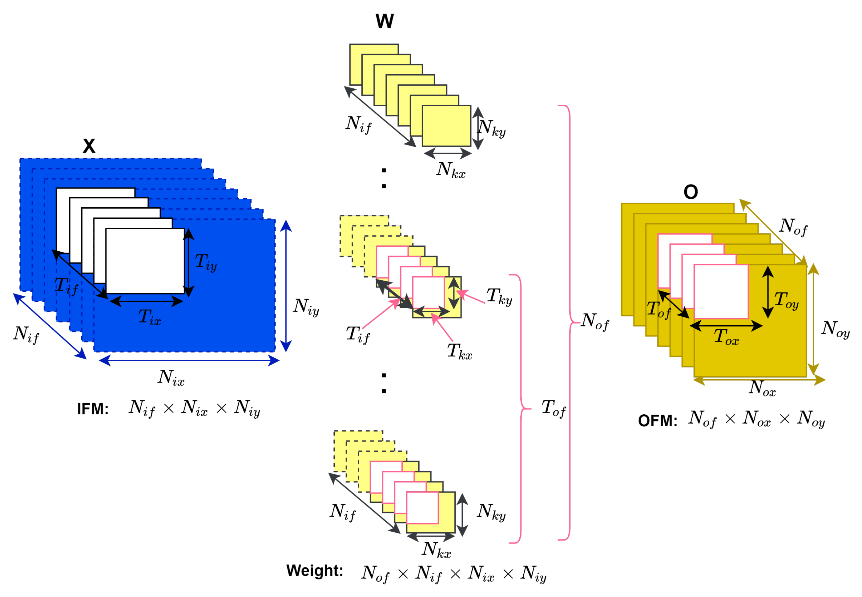
3.2. Convolution Layer

The convolution layer is the core and computation-intensive part of CNN-based networks, reportedly taking over 90% of the network’s execution time [11]. Consider Figure 2 showing a particular convolutional layer with an input feature map (IFM) tensor of shape X = N i f × N i x × N i y , weight kernel of shape W = N o f × N i f × N k x × N k y and an output feature map (OFM) of shape O = N o f × N o x × N o y . The subscripts o f , o x , o y stand for the output feature map depth, row (height), and column (width) of the output feature map. Similarly, subscripts i f , i x , i y serve the same purpose but for the input feature map. We will stick to these notations throughout the paper for consistency.
Convolution is thus a process of repeated multiply and accumulate operations of a pre-trained weight kernel of shape N i f × N k x × N k y against an input feature map or an input image of a shape N i f × N i x × N i y by striding the weight kernel across the surface of the input with a stride of size S. This process is repeated N o f times—once for each of the N o f different kernels yielding an output of size N o f × N o x × N o y . The Equation (1) mathematically describes this convolution process.
O [ m ] [ x ] [ y ] = i = 0 K 1 j = 0 K 1 n = 0 N 1 ( X [ n ] [ x i ] [ y i ] × W [ m ] [ n ] [ i ] [ j ] ) + B [ m ]
where
x i = x × S + i
y i = y × S + j
K = N k x = N k y , N = N i f
m { 0 , N o f } , x { 0 , N o x } , & y { 0 , N o y }
Equation (1) assumes that the width and height of the weight kernels to be equal as is the case with YOLOv2 and almost all modern CNN-based networks. The relationship between the input and output feature map width and height is also determined using Equations (2) and (3). The P in the equation stands for the zero-padding of the input feature map so that the resulting output feature map will have either a ‘valid’ or ‘same’ shape. Valid is for when the input is not padded, meaning that P = 0 and the output will have a slightly shorter width and height compared to the input feature map, whereas in the ’same’ convolution, the output and input will have the same width and height and hence P is different from zero.
N o x = N i x + 2 P N k x S + 1
N o y = N i y + 2 P N k y S + 1
The pseudocode in Listing 1 demonstrates that the unoptimized convolution will have six nested loops for a single-input image or input feature map. From this, we can understand that there are N o f × N i f × N o x × N o y × N k x × N k y total multiply–accumulate (MAC) operations for every convolution layer. The X, W, B and the O in the pseudocode stands for IFM, weight, bias and OFM, respectively.
Listing 1. Unoptimized standard convolution pseudocode for batch-size = 1.
 1for (m=0; m<Nof;m++){
 2   for (y=0; y<Noy;y+=S){
 3     for (x=0; x<Nox;x+=S){
 4       for (n=0; n<Nif;n++){
 5         for (ky=0; ky<Nky;ky++){
 6           for (kx=0; kx<Nkx;kx++){
 7             O[m][x][y]+= X[ni][S*x+kx][S*y+ky] * W[m][n][kx][ky];
 8           }
 9         }
10       }
11       O[m][x][y] += B[m];
12     }
13   }
14 }

3.3. Pooling Layer

Another common layer type in a modern object detection CNN network is a pooling layer. A pooling layer reduces the preceding layer’s spatial dimensions and facilitates the prospect of a deeper network. Moreover, it also increases the network’s translation invariance by omitting pixels from a feature map through either maximum or average pooling. It also minimizes, to a lesser extent, network overfitting to the training dataset. It is worth noting that the pooling layer has no trainable parameter. Accordingly, more recent state-of-the-art models utilize alternative layers such as up-sampling and down-sampling to enable learned pooling. The pooling layer, particularly the max-pooling layer, has three nested loops as depicted in pseudocode Listing 2. — Solomon: I believe the english is correct and the meaning after and before the change are the same.
Listing 2. Original max-pooling pseudocode.
 1for (no=0; no<Nof;no++)
 2   for (y=0; y<Noy;y+=S)
 3     for (x=0; x<Nox;x+=S)
 4       O[no][x][y]=Max(X[n0][x:x+S][y:y+S])

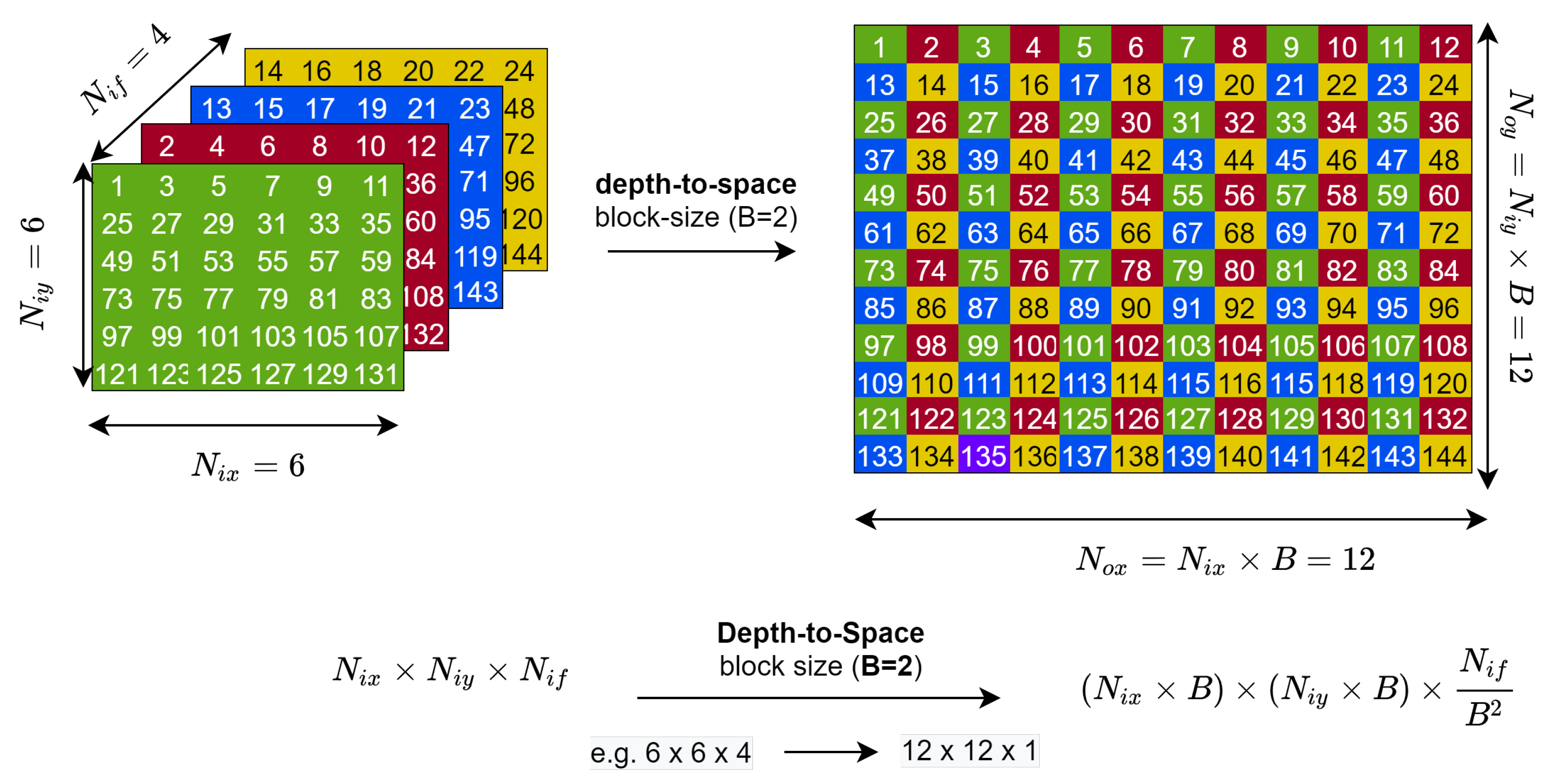
3.4. Depth-to-Space or Space-to-Depth Reorganization Layer

The other layer type in YOLOv2 is a reorganization layer, known in the TensorFlow framework as the space-to-depth or depth-to-space layer. These reorganization processes reshuffle the previous layer’s feature maps into either channel-wise deeper feature maps, shown in Figure 3, or spatially wider feature maps, shown in Figure 4. Reorganization is commonly performed for the facilitation of the concatenation of two or more layers of different shapes. In our case, layer 27 of YOLOv2 is a space-to-depth reorganization of layer 26 with a block-size of B = 2 × 2 (seen Figure 1 or Table 1). The following layer, layer 28, concatenates the output of layers 24 and 27. Note that, in the reorganization layer, there are no learned or learnable parameters (or hyperparameters).

3.5. Batch Normalization Layer

The batch normalization layer is inter-layer data normalization, which differs from input normalization during pre-processing, to accelerate object detection training convergence by minimizing internal variance among layers. This usually comes after the convolution layer, just before the non-linear activation layer. In short, batch normalization involves four mathematical steps: (1) calculating the mean of an output of the convolution layer Equation (4); (2) calculating the variance of an output of the convolution layer, Equation (5); (3) normalizing the convolution output so that its mean and variance become 0 and 1, respectively, Equation (6); and finally (4) scaling and shifting the normalized data using learned hyperparameters γ and β , Equation (7). The value after the fourth step will be input to the next layer, which is going to be Leaky Relu in the YOLOv2 object detector.
μ B 1 m i = 1 m x i
σ B 2 1 m i = 1 m ( x i μ B ) 2
x i ^ x i μ B σ B 2 + ϵ
y i γ x i ^ + β B N γ , β x i

3.6. Leaky Relu Activation Layer

In YOLOv2, the Leaky Relu activation function given by Equation (8) is used for the non-linear transformation of the feature map pixels yielded from the preceding layer—in our case, the batch normalization layer.
y = x , if x 0 α x , o t h e r w i s e , w h e r e α [ 0 , 1 ]

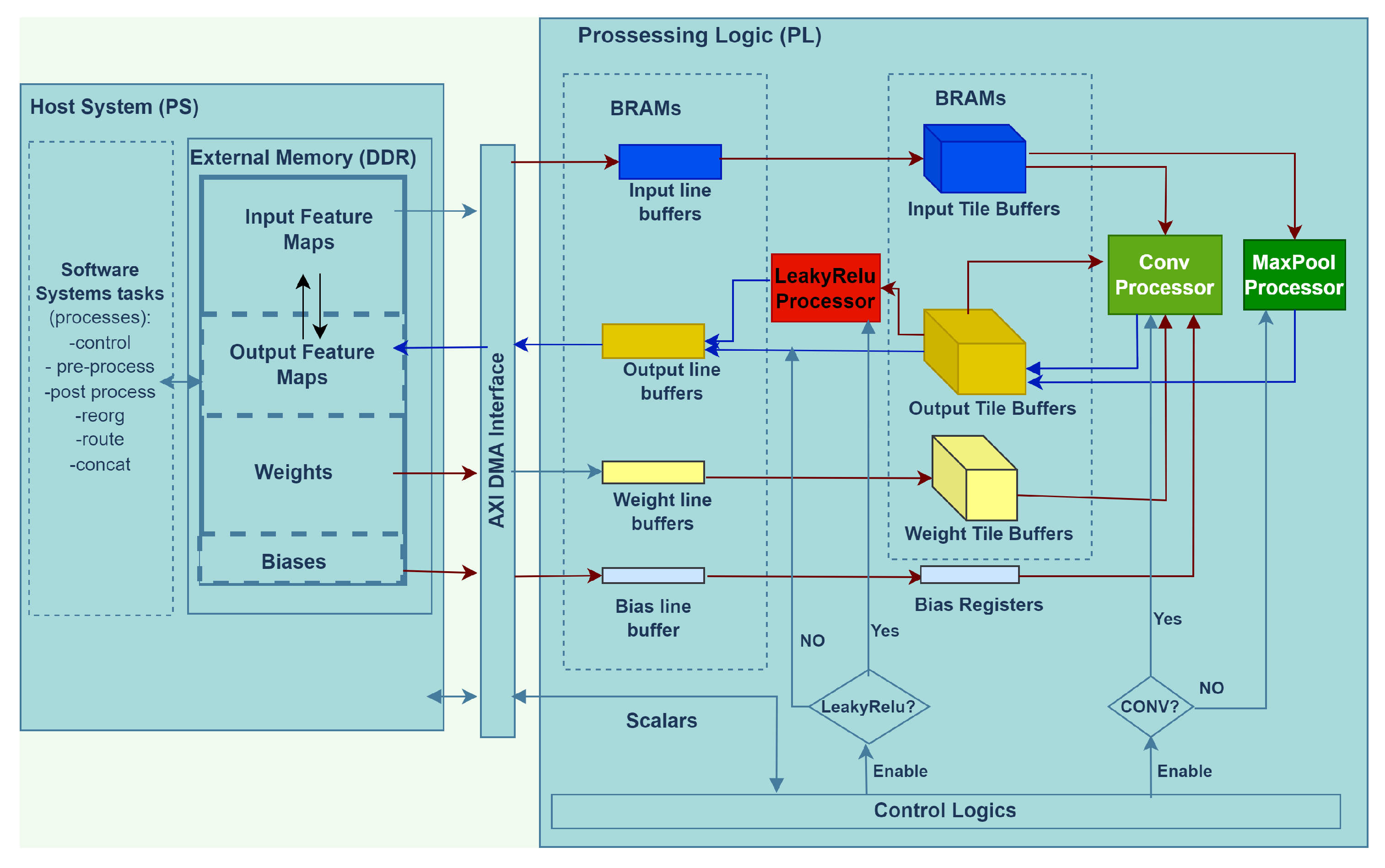
4. The Proposed Hardware Acceleration of Object Detection Inference

4.1. General Overview

We propose a hardware–software coprocessing dual system where the computation-intensive layers, namely all convolution, max-pooling, and activation layers, are offloaded to an FPGA (Programmable Logic or PL) to benefit from FPGA’s parallelism capabilities. In contrast, layers that are non-computation oriented, such as the reorg and route layers, are processed by a processor onboard our test system (processor system or PS), typically an ARM processor. Moreover, the PS supervises the overall control of the detection network’s end-to-end flow, including the pre- and post-processing stages.
Figure 5 shows the overall architecture of our proposed object detection accelerator. As seen from the figure, a pre-trained YOLOv2 weight, bias and input-images are stored on a DDR memory of the host system which also contains the processor and the software accelerated portions of our object detection network. All contents of the DDR memory are 16-bit quantized. An AXI-DMA interface connects the host systems’ PS and DDR memory with the PL side’s custom accelerator, where the heavy-duty arithmetic of the convolution, max-pooling and Leaky Relu are executed. In general, the core features of our hardware-accelerated object detection inference includes:
  • A highly hardware resource-efficient and optimized convolution and max-pool processors based on standard optimization techniques such as loop tiling, unrolling and convolution loop reordering;
  • Per-layer dynamic 16-bit data quantization of the weight, bias, IFM and OFM;
  • Double buffering-based memory read, computation and writeback for smooth convolution acceleration, one that avoids memory access from becoming its bottleneck.
We shall then discuss these features of our design choice one by one in detail.

4.2. Loop Tiling

As discussed in earlier sections, current state-of-the-art object detectors are deep and have millions of trainable parameters and tens or hundreds of megabytes. As a result, breaking the inputs and outputs into FPGA-manageable chunks of blocks is an inevitable part of the hardware-accelerated implementation of these state-of-the-art models. Recall how Figure 2 shows a particular convolutional layer with an input tensor of shape X = N i f × N i x × N i y , weight kernel of shape W = N o f × N i f × N k x × N k y and an output feature map (OFM) of shape O = N o f × N o x × N o y . To better illustrate loop tiling, we return to our earlier Figure 2; however, this time, we include the loop tiling information, as seen in Figure 6, with the white-shaded regions indicating the tile sizes.
The two following equations give the relationship between the input and output tiles’ width and height:
T i x = ( T o x 1 ) S + N k x
T i y = ( T o y 1 ) S + N k y
Some prior works relied on custom-built algorithms such as roofline modeling to determine the optimum tile size parameters. Instead, we opt for a simplistic but intuitive strategy or criterion to specify the appropriate tile sizes that guarantee data reuse and optimized resource utilization. Our simplistic yet intuitive strategy is based on the following assumptions or criteria:
  • For the efficient utilization of the scarce on-chip memory of the FPGA (that is, the BRAM or block random access memory), the max-pooling and convolution layers shall use the same memory blocks for buffering. This is possible since the two layers never happen simultaneously but one after another. Thus, we enforce resource-sharing among the two core processing elements.
  • The bigger the data that we can fit on the on-chip memory through burst transfer is, the better it is to avoid frequent external memory access because external memory access is relatively slow compared to the actual computation.
  • Determining the buffer sizes should not be solely based on the layers with the biggest width, height and/or depth. Instead, tile sizes should be a common divisor of all or most layers so as not to assign excessively-big buffers for most of layers, thereby wasting on-chip memory and energy or excessively small buffers, increasing external memory transaction frequencies.
In YOLOv2, the convolution stride ( S ) equals one, whereas the max-pooling stride is two. Based on our strategy of using shared buffers for max-pooling and convolution and the fact that max-pooling requires a buffer size almost twice that required by convolution for the same output tile of size T o f × T o x × T o y , we base our tile size selection based on the demands of max-pooling layers. By substituting the value of S = 2 , we can then rewrite Equations (9) and (10) as follows:
T i x = ( T o x 1 ) × 2 + 2 = 2 × T o x
T i y = ( T o y 1 ) × 2 + 2 = 2 × T o y
Table 2 shows the tensor shapes, corresponding tile sizes and the number of external memory read- or write-access iterations. The number of BRAMs (on-chip buffers) required for each tile is calculated as:
N u m b e r o f B R A M p e r T i l e = T i l e S i z e × D a t a W i d t h S i z e o f O n e B R A M
However, depending on the convolution loop arrangement and array partitioning, the actual required BRAM would be larger than what we obtain by Equation (13). Moreover, as seen from the overall architecture in Figure 5, each tile has an associated line buffer for burst transfer, adding up the total BRAM utilization of the hardware solution.
Finally, according to first of the aforementioned criteria, the input and output tile buffer sizes (only the width and height, T i x and T i y for input tile, and T o x and T o y for output tile) are determined based on the max-pooling layer and Equations (11) and (12). However, T i f and T o f ’s choices require considering the implemented custom convolution accelerator and available resources, such as the DSPs and logic cells and the aforementioned criteria. We analyzed the YOLOv2 layers for setting T i f and observed that N i x ’s minimum and maximum values are 3 and 1280, corresponding to the input and layer 29, respectively. Similarly, the minimum and maximum values of N o f are 32 and 1024, respectively. Although we would like to assign as big a buffer as possible for the tiles according to the second of the aforementioned criteria, we should also respect condition 3, i.e., assigning a suitable buffer for all the layers of YOLOv2. Accordingly, we selected T i f = 4 , which is neither excessively larger than the minimum nor excessively small, causing frequent memory access. However, T o f can be set to 32 or more based on the available BRAM and DSP, considering we designed a convolution processor with T i f × T o f simultaneous MACs (explained under Section 4.5). The final tile size choices of our implementation are discussed in Results and Discussions section, Section 5.

4.3. Double Buffering

To further increase the throughput of our hardware accelerator, we use the concept of double buffering, also called ping-pong buffering. Double buffering helps to overlap memory read, compute, and writeback operations, solving the memory access bottleneck. It also requires twice as much memory as implementation without double buffering, resulting in high resource consumption. We implement double-buffering using an approach similar to that in [19]. We implement a two-stage ping-pong: one for reading input tiles (weight and input feature maps) and another for writing back the final convolution results. As seen in Figure 7, during the first iteration of the innermost loop, the input feature map and weight tiles are brought to their corresponding buffers (IFM_buffer0, Weight_buffer0). In the next iteration, while the convolution processor simultaneously performs a convolution operation on the earlier inputs, the next batch of inputs are loaded onto the second set of corresponding buffers (IFM_buffer1, Weight_buffer1). The convolution results are kept on either OFM_buffer0 or OFM_buffer1 until the innermost loop is completed. The Algorithm 1 shows the ping-pong process more precisely and briefly. Two Boolean variables (pingpong_ifm, pingpong_ofm) control the double buffering sequencing, while the input read, compute and output writeback stages are controlled by loop iteration checks, omitted from the pseudocode for brevity. In general, there are N i f T i f + 1 input tile reads for each output tile writeback and in total there are N o f T o f + 1 writebacks.
Algorithm 1: Illustration of our double-buffering implementation
Electronics 11 01827 i001

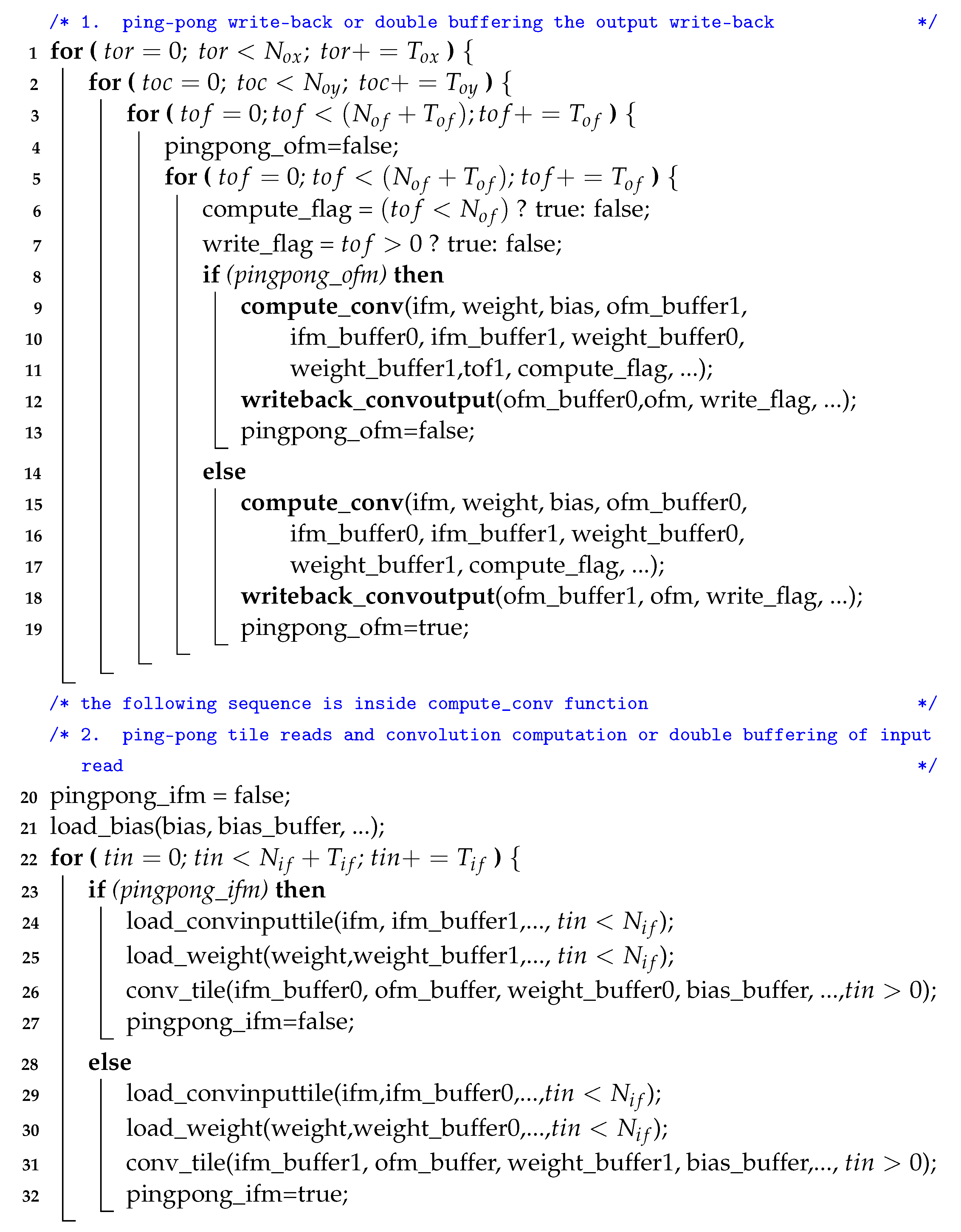
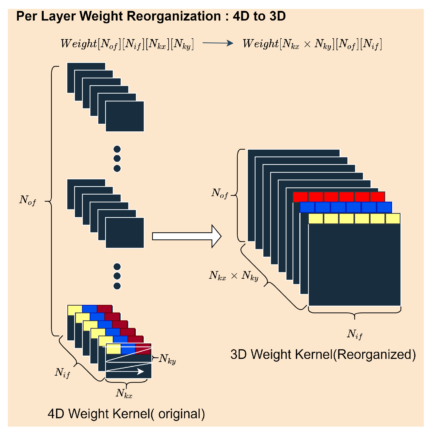
4.4. Data Quantization and Weight Reorganization

As state-of-the-art object detections model sizes steadily increase to achieve increased performance, the network becomes slower and more resource-demanding. Consequently, the model quantization of trained weights and biases has become an integral part of hardware acceleration implementation. As discussed in our Related Works section, extreme quantizations yield a high-speed model. However, the accuracy loss is usually not worth the speed gain for most real-world application areas of computer vision since a detector should be not only fast, but fast as well as accurate. As a result, instead of extreme quantization, we opted for the 16-bit quantization of the trained weights, biases, and input feature maps.
Quantization converts the trained network parameters from the de facto 32-bit floating-point precision into an m b i t fixed-point precision binary string. The quantized model will be lighter in size and hence faster. To mathematically describe the quantization process, let us consider W f l o a t 32 as the 32-bit (also called single) precision IEEE 754 standard number, and its 16-bit quantized equivalent as W q u a n t 16 . To quantize W f l o a t 32 into W q u a n t 16 , we first need to determine an integer Q, such that the integer part of W f l o a t 32 could be represented by n ( m Q ) bits, and in our case m is 16 since we target 16-bit quantization. For example, if W f l o a t 32 = 3.24 , the integer part is +3, a small number that can be represented by n = 2 bits. However, considering the potential of W f l o a t 32 as negative, we leave at least three bits for the portion before the decimal point. This leaves our Q to be 13. Once the Q value is determined, the quantized W q u a n t 16 is calculated as:
W q u a n t 16 = W f l o a t 32 × 2 Q
In our example, substituting the Q value gives W q u a n t 16 = 3.24 × 2 13 = 26542 . Using Equation (15), one can reverse the quantized value back into floating precision though a slight difference is expected due to rounding. In fact, the quantization error can also be calculated using the Equation (16).
W f l o a t 32 = W q u a n t 16 × 2 Q
e r r o r = W f l o a t 32 W f l o a t 32
Similarly to the above explanation, we implemented the weight, input, and output feature map and bias quantization using 16-bit per-layer dynamic quantization. For example, the 16-bit dynamic weight quantization is presented in the pseudocode listing of Algorithm 2. Furthermore, after quantizing, we reorganized the weight tensor from its original 4D shape of N o f × N i f × N k x × N k y , as shown in Figure 2, to a 3D shape N k x y × N o f × N i f , as seen in Figure 8. N k x y is the product of the width and height of the kernel, that is N k x × N k y = N k x y . Hereafter, in our hardware accelerator design, we refer to the weight tensor in this 3D shape rather than its original 4D shape. The quantized weight tensor is saved in the DDR memory in the order of tiles that the convolution processor expects so that a continuous high-speed burst transfer is made to the on-chip buffer.
Algorithm 2: Per-layer 16-bit dynamic quantization of weight
Electronics 11 01827 i002

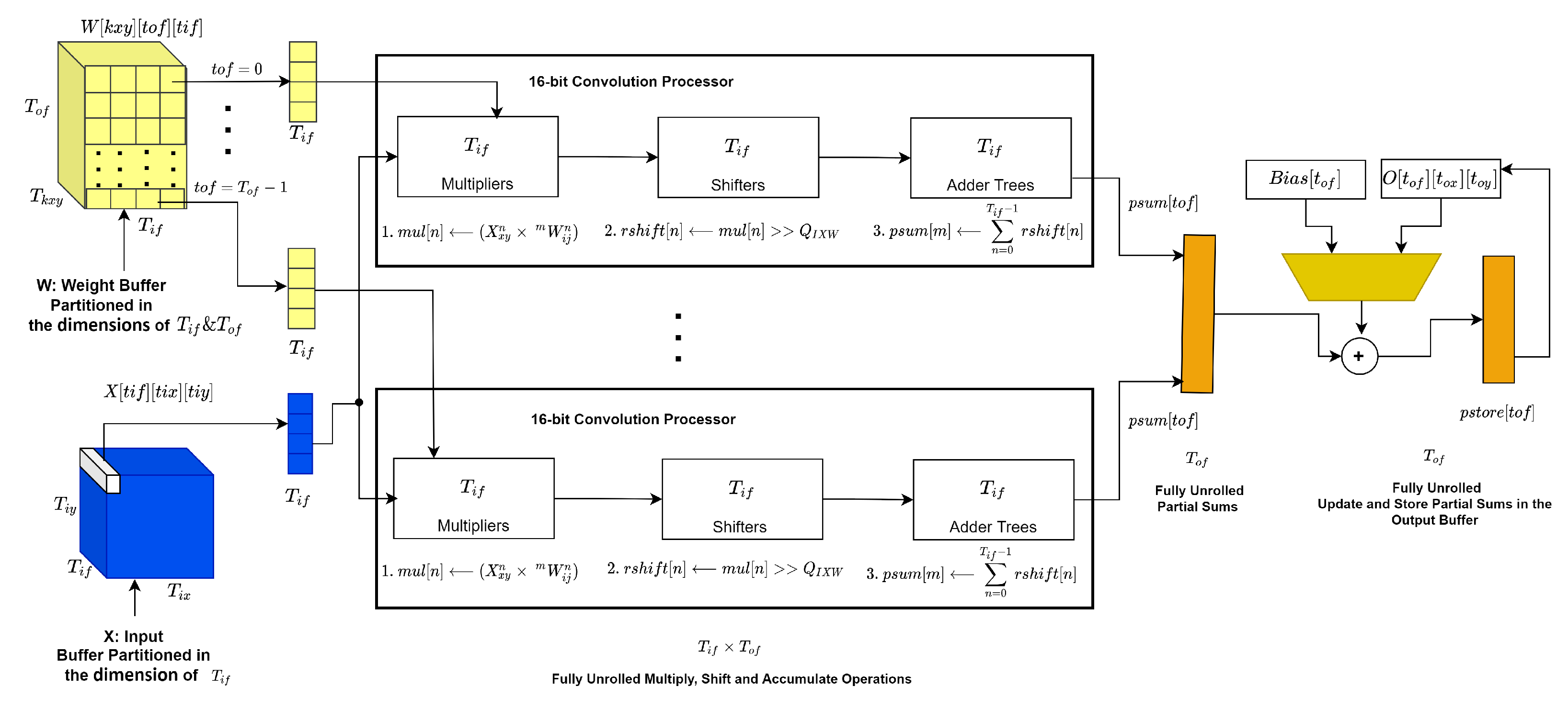
4.5. Convolution Processor

The convolution layer is the most resource-demanding and computation-intensive part of the object detector CNN network. As shown in Listing 1, the unoptimized convolution has six nested loops, even though they must not always be in the same sequence. We use standard loop tiling, unrolling, and interchange to design an optimized hardware-accelerated version of the convolution. Convolution in fixed-point precision is no longer only an MAC (multiply and accumulate); instead, it is multiply, right shift, and accumulate. Thus, we like to refer to it as MSA operations, not MAC. The amount of right shift is calculated from the Q values of the input quantization Q X , weight quantization Q W , and an intermediate value Q I . We will explain this better with a diagrammatic depiction. Figure 9 shows the smallest processing element (PE) unit of our fixed-point convolution implementation. In the figure, two 16-bit numbers with different Q, that is, Q X for the input pixel and Q W for the weight ’pixel’ pass through the multiplier followed by the right-shift operator and then the accumulator. Had it been a floating-point precision, the decimal point would have been placed at Q X W of the resulting product. However, since this is a fixed-point precision operation, we replace the decimal point with a two’s power division or right-shift. Right shift with Q = Q X W would completely discard the fractional points from the result of the product. Instead, we perform a right-shift operation using Q = Q I X W = Q X W Q I . The best Q I for 16-bit quantization is Q I = 15 since this value leaves the maximum room for the decimal parts without completely discarding the fractional value. One might refer to this as an intermediate or partial sum quantization. Note that we also perform an output quantization after Leaky Relu to convert the 32-bit partial sum back to 16-bit and write back the result of the output quantization to the DDR memory through a pipelined burst-transfer.
In general, our convolution processor has T o f × T i f fully unrolled multipliers followed by fully unrolled T o f × T i f right-shift operation and T o f × T i f partial adder trees fully unrolled in the T o f dimension and pipelined with the smallest possible initiation interval (II = 1) in T i f dimensions. The overall architecture of the designed convolution processor is shown in Figure 10.
Given the overall design of the convolution processor, the next target was to determine the optimum sequence of the nested loops of convolution. An optimum design for the convolution loops needs to minimize the number of partial sum store and read operations, utilize fewer logic cells, and take full advantage of the redundant onboard resources of the FPGA and DSPs for parallelism, all while being energy efficient. To this point, we tested many possible arrangements of the convolution nested loops, and we finally came down to two contending choices given the limited resources of our development boards. These two competing implementations of the convolution compute function, also briefly mentioned under the double buffering section (see Algorithm 1), are given by Listings 3 and 4. In the first version, we obtain the lowest partial sum read and write. However, the convolution kernels are not fixed for all convolution layers. Instead, they alternate between 1 × 1 and 3 × 3 in YOLOv2. As a result, placing the loops labeled _nki and _nkj in the middle of the nested loops increases the iteration control hardware, consumes more logic cells and increases latency. We compared it against the second version given by Listing 4 and found that Listing 3 is three times slower. Our final optimized convolution accelerator was thus chosen to be the one mentioned in Listing 4.
To summarize some of the core features of our convolution accelerator, we mention the following key points:
  • Per block (tile), the convolution compute latency is given by the Equation (17) below:
    ( N k x × N k y × T o x × T o y + C ) × 1 F c l k
    C stands for the ’constant’ referring to the number of cycles needed to perform the fully unrolled inner operations commented 1–4 in the pseudocode Listing 4 and loop iterations control logic. In our implementation, C is equal to either 13 or 21 based on the kernel types, 1 × 1 or 3 × 3 , respectively. F c l k stands for clock frequency.
  • The total compute latency for a convolution layer is calculated as:
    N o f T o f × N o x T o x × N o y T o y × N i f T i f × ( N k x × N k y × T o x × T o y + C ) × 1 F c l k
  • The total number of multiply, shift and accumulate operations per convolution layer is calculated as:
    3 × N o f T o f × N o x T o x × N o y T o y × N i f T i f × ( N k x × N k y × T o x × T o y × T o f × T i f )
Listing 3. Version 1: Optimized convolution pseudocode on input and weight tile.
 1 int32_t lineinput[Tif];
 2 int32_t pmul[Tif];
 3 int32_t rshift[Tif];
 4 int32_t psum[Tof];
 5 int32_t pstore[Tof];
 6 _trconv:for(tr = 0;tr < min(Tox,Nox);tr++){
 7   _tcconv:for(tc = 0;tc < min(Toy,Noy);tc++){
 8     //1. clear
 9     _pmulclear:for(tm = 0;tm <Tof;tm++){
10       #pragma HLS unroll //PIPELINE II=1
11       psum[tm]=0;
12     }
13     //2. compute multiply, shift and accumulate
14     _nkiconv:for(i =0;i < Nkx; i++){
15       _nkjconv:for(j = 0;j < Nky; j++){
16         tix = tr*Kstride + i;
17         tiy = tc*Kstride + j;
18         tkxy = i*Ksize + j;
19         _tnminiInput:for(tn = 0;tn <Tn;tn++){
20           #pragma HLS unroll
21           lineinput[tn]= X[tn][tix][tiy];
22         }
23         _tmconv:for(tm = 0;tm < Tof;tm++){
24           #pragma HLS unroll
25           _tnconv1:for(tn = 0;tn <Tif;tn++){
26             #pragma HLS unroll
27             pmul[tn]= W[tkxy][tm][tn]*lineinput[tn];
28           }
29           _tnconv2:for(tn = 0;tn <Tif;tn++){
30             #pragma HLS unroll
31             rshift[tn]= pmul[tn]>>Qixw;
32           }
33           _tnconv3:for(tn = 0;tn <Tif;tn++){
34             #pragma HLS unroll
35             psum[tm]+= rshift[tn];
36           }
37         }
38       }
39     }
40     //3. update
41     _psupdate:for(tm = 0;tm <Tof;tm++){
42       #pragma HLS unroll
43       if(n==0){
44         pstore[tm] = B[tm] + (psum[tm]);
45       }
46       else{
47         pstore[tm] = O[tm][tr][tc]+ (psum[tm]);
48       }
49     }
50     //4. store
51      _psstore:for(tm = 0;tm <Tof;tm++){
52       #pragma HLS unroll
53        O[tm][tr][tc]= pstore[tm];
54     }
55   }
56 }
Listing 4. Version 2: Optimized convolution pseudocode on input and weight tile.
 1 int32_t mul[Tif];
 2 int32_t rshift[Tif];
 3 int32_t psum[Tof];
 4 int32_t pstore[Tm];
 5 _nkiconv:for(i =0;i < Nkx; i++){
 6   _nkjconv:for(j = 0;j < Nky; j++){
 7     _trconv:for(tr = 0;tr < min(Tox,Nox);tr++){
 8       _tcconv:for(tc = 0;tc < min(Toy,Noy);tc++){
 9         //1. clear partial sum
10         _pmulclear:for(tm = 0;tm<Tof;tm++){
11           #pragma HLS unroll
12           msa[tm]=0;
13         }
14         //2. compute multiply, shift and accumulate
15         _tmconv:for(tm = 0;tm < Tof;tm++){
16           #pragma HLS unroll
17           //2.1 multiply
18           _tnmultiply:for(tn = 0;tn <Tif;tn++){
19             #pragma HLS unroll
20             mul[tn]= W[i*Nkx+j][tm][tn]*
21             X[tn][tr*S + i][tc*S + j];
22           }
23           //2.2 right-shift for decimal point consideration
24           _tnshift:for(tn = 0;tn <Tif;tn++){
25             #pragma HLS unroll
26             rshift[tn]= mul[tn]>>Qixw;
27           }
28           //2.3 accumulate to partial sum
29           _tnaccumulate:for(tn = 0;tn <Tif;tn++){
30             #pragma HLS unroll
31             psum[tm]+= rshift[tn];
32           }
33         }
34         //3. update stored partial sum
35         _pupdate:for(tm = 0;tm <Tof;tm++){
36           #pragma HLS unroll
37           if(i ==0 && j==0 && n==0){
38             pstore[tm] = B[tm] + (psum[tm]);
39           }
40           else{
41             pstore[tm] = O[tm][tr][tc]+ (psum[tm]);
42           }
43         }
44         //4. store partial sum
45         _pstore:for(tm = 0;tm <Tof;tm++){
46           #pragma HLS unroll
47           O[tm][tr][tc]= pstore[tm];
48         }
49       }
50     }
51   }
52 }

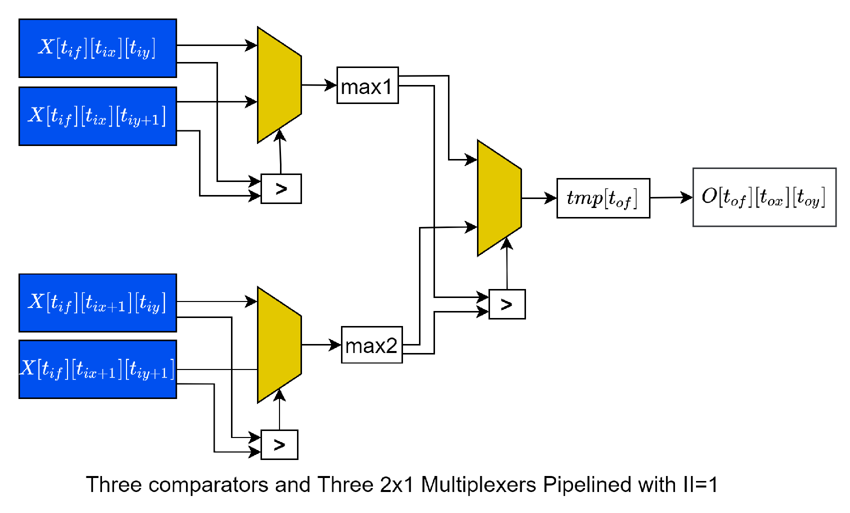
4.6. Max-Pooling Processor

As explained earlier, YOLOv2 has five 2 × 2 max pool layers with a stride of S = 2, each following a Leaky Relu activation layer. Although max-pooling does not have an intensive computation complexity, it could benefit from FPGA’s parallelism since it works on the individual ’pixels’ of the input feature maps. Likewise, we designed a pipelined max-pool accelerator with three selectors and comparators, as seen in Figure 11. The input tile size for max-pool has the same depth as the convolution’s input feature map depth, which is T i f . The pseudocode for the hardware-accelerated max-pool on an input tile is given in Listing 5.
Listing 5. Optimized max-pool processor for 2 × 2 kernel stride.
 1 int16_t tmp[Tif];
 2 int16_t tmp1, tmp2,tmp3, tmp4, max1,max2;
 3 _toxmax:for(_tox = 0;_tox < min(Tox,Nox);_tox++){
 4   _toymax:for(_toy = 0;_toy < min(Toy,Noy);_toy++){
 5     _tofmax:for(_tof = 0; _tof < min(Tif,N_{if}); _tof++){
 6       #pragma HLS PIPELINE II=1
 7       tmp1=X[_tof][_tox*S][_toy*S];
 8       tmp2=X[_tof][_tox*S][_toy*S+1];
 9       max1 = (tmp1 > tmp2) ? tmp1 : tmp2;
10
11       tmp3=X[_tof][_tox*S+1][_toy*S];
12       tmp4=X[_tof][_tox*S+1][_toy*S+1];
13       max2 = (tmp3 > tmp4) ? tmp3 : tmp4;
14
15       tmp[_tof] = max1 > max2 ? max1 : max2;
16
17     }
18     maxstore:for(_tof = 0; _tof < min(Tif,Nif); _tof++){
19       #pragma HLS PIPELINE II=1
20       O[_tof][_tox][_toy] = tmp[_tof];
21     }
22   }
23 }

4.7. Leaky Relu Hardware Processor

In YOLOv2, following every convolution layer comes a Leaky Relu activation, except for the last convolution layer, which is linear activation. The floating-point equivalent of Leaky Relu was discussed earlier and described using Equation (8). In the equation, the constant α is set to 0.1 for YOLOv2, and since we are working on 16-bit fixed precision, we convert the multiplying α = 0.1 into 16-bit fixed-point quantized binary string using Q = 15 . The quantized α is equivalent to base ten 32768 or hex 0 x C C C . In general, the hardware equivalent of Leaky Relu is implemented using the following expression:
 1   tmp_out[i]= (tmp_in[i] < 0) ? (tmp_in[i]*0xccc)>>15 : tmp_in[i];
where t m p _ i n is a pixel from the output buffer, and t m p _ o u t is the ’pixel’ after passing through a Leaky Relu processor. The overall architecture can be seen in Figure 5 for clarity.

5. Results and Discussions

Although we mainly discussed the FPGA implementation of object detection using YOLOv2, our implementation can be easily configured for other types of similar networks such as DenseYOLO and DDGNet, which are even more lightweight and accurate. We implemented the proposed hardware accelerator using C++, Vitis HLS 2021.1, and Vivado 2021.1. The convolution, max pooling, and Leaky Relu layers are implemented as FPGA accelerated functions. In contrast, the remaining space-to-depth reorganization, concatenation, and route layers, including the input and output pre-processing and post-processing, are performed on the ARM processor onboard our test boards. Following every convolution layer, the batch normalization layer computations were already included in generating the quantized weights and biases, avoiding the need to construct a hardware-equivalent one.
We targeted two Xilinx boards, namely ZYNQ-7000 SoC, specifically Z-7020CGL484-1 and ZCU102 development boards from ZYNQ UltraScale+ MPSoC for the implementation of YOLOv2-based object detection inference. As seen in Table 3, the Z-7020CGL484-1 has minimal resources compared to ZCU102. Since double buffering requires twice as many on-chip buffers than an implementation without double-buffering, we had to use different tile sizes for the two boards.
Table 4 shows our tile-size design choices and implementation clock frequencies for the two boards. The table also shows the total resources consumed by our hardware accelerator. Both implementations required resources well under the range of the design guidelines of the boards, proving efficient implementation. We also achieved a clock frequency of 150 MHz and 300 MHz for ZYNQ-7020 and ZCU-102, respectively. By combining Equations (18) and (19), we calculated an overall throughput (giga operations per second (GOP/S)) of 51.06 GOP/S and 184.06 GOP/S for ZYNQ7020 and ZCU102, respectively. Another helpful metric called DSP efficiency, as coined by [23,29], measures how efficiently the DSPs in the convolution accelerator are utilized. These define DSP efficiency as a ratio of effective operation or the actual operation that the layer requires over the actual number of operations that the implemented convolution processor performed. According to this definition, our tile size choices and accelerator loop arrangement, the DSP efficiency is 100% for both boards, except for the first and last YOLOv2 layers. Such a high DSP efficiency is partly because of the uniformity of YOLOv2’s layers.
Furthermore, we also analyzed the per layer execution latency of YOLOv2 layers for the two boards, as shown in Figure 12 for the two implementations. For ZYNQ-7020, the total execution time for end-to-end YOLOv2 object detection inference processing takes 0.868 s. In contrast, the ZCU102 only takes 0.244 s for a single 416 × 416 RGB image of the COCO object detection dataset. From the figure, layer 29 of YOLOv2 is the slowest, taking up to 26 and 104 ms on ZCU102 and ZYNQ-7020, respectively. On a personal laptop computer of Intel(R) Core i7-7700HQ CPU @ 2.80GHz 16GB RAM Ubuntu 20.04, our YOLOv2 inference takes a maximum of 7 s to infer all bounding boxes and object classes on a single-core single-thread CPU for a single batch of image from COCO dataset with size 416 × 416. Thus, our FPGA implementation accelerates YOLOv2 inference by up to 28.68 and 8.06 times for ZCU102 and ZYNQ-7020, respectively, compared to the software version on the personal laptop. All this consumes 2.78 watt for ZYNQ-7020 and 5.376 watt on ZCU102, evidencing how our implementation is much more efficient than the other implementations we compared it with.
We compared our YOLOv2 object detection inference implementation with other closely related works, and Table 5 summarizes the comparison using different metrics or criteria. Although there are many FPGA-based inference accelerations, the main reasons we picked these sample references to compare against our work are that (1) these works are recent; (2) all are one-stage object detection inference accelerations (4) based on YOLO versions and 1 based on SSD); and (3) all are abundantly cited prior works with close resemblance to our approach. As the table shows, our implementation maintains the most resource and power-efficient performance while still having a commendable GOP/S at a frequency as high as 300 MHz and higher DSP efficiency. Moreover, though some entries in the table never reported their accuracy performance, our implementation of YOLOv2 inference on the Pascal VOC 2007 dataset at a resolution of 416 × 416 yielded an mAP of 76.21%, a little below the baseline 32-bit floating precision’s 76.8% mAP of the original YOLOv2. The 16-bit quantization of the data and the fixed-point arithmetic of our custom convolution processor explained by Figure 9 played a significant role in increasing the mean average precision of our accelerator.
In general, we obtained an efficient hardware-acceleration design scheme that preserves the scarce and precious resources of an FPGA while yielding higher performance at low-energy consumption. We used a shared double-buffered on-chip buffer to conserve memory and avoid memory access becoming a bottleneck to our hardware convolution accelerator. Compared to [23] consuming 100 Watt energy and approximately fifteen times more DSPs than our implementation, we achieve a commendable 0.244 s in execution latency of YOLOv2 at a mere 5.376 Watt and 291 DSPs utilized. Given the fact that we used a 16-bit fixed-point precision, there is a reasonable prospect for our implementation to achieve real-time acceleration by changing our quantization strategy to an 8-bit or mixed precision as well as save more resources and power while still managing to maintain the minimum possible loss in detection accuracy.
Finally, Figure 13 shows the sample output of our hardware accelerator performing impeccably well with high accuracy as good as the full 32-bit floating-point precision implemented on our laptop.

6. Conclusions

This paper implemented the YOLOv2 inference accelerator on two Xilinx development boards with varying available resources and achieved a resource- and power-efficient accelerator. Our best-performing implementation achieved a commendable throughput of 184 GOP/S and 0.244 s inference time per image using 16-bit fixed point dynamic quantization and consuming only 5.376 watts. In future work, we intend to test different quantization strategies without compromising accuracy and energy efficiency so that our implementation achieves real-time inference.

Author Contributions

Conceptualization, S.N.T. and E.-B.B.; methodology, S.N.T.; software, S.N.T.; validation, S.N.T. and E.-B.B.; formal analysis, S.N.T.; investigation, S.N.T.; resources, S.N.T.; data curation, S.N.T.; writing—original draft preparation, S.N.T.; writing—review and editing, S.N.T.; visualization, S.N.T.; supervision, E.-B.B.; project administration, E.-B.B.; funding acquisition, E.-B.B. All authors have read and agreed to the published version of the manuscript.

Funding

This research received funding from Ethiopian Ministry of Science and Higher Education (MOSHE) and French Government for promotion of higher education and research.

Institutional Review Board Statement

Not applicable.

Informed Consent Statement

Not applicable.

Data Availability Statement

Not applicable.

Conflicts of Interest

The authors declare no conflict of interest.

References

  1. Krizhevsky, A.; Sutskever, I.; Hinton, G.E. Imagenet classification with deep convolutional neural networks. Adv. Neural Inf. Process. Syst. 2012, 25, 1097–1105. [Google Scholar] [CrossRef]
  2. Redmon, J.; Divvala, S.; Girshick, R.; Farhadi, A. You only look once: Unified, real-time object detection. In Proceedings of the IEEE Conference on Computer Vision and Pattern Recognition, Las Vegas, NV, USA, 27–30 June 2016; pp. 779–788. [Google Scholar]
  3. Lin, T.Y.; Goyal, P.; Girshick, R.; He, K.; Dollár, P. Focal loss for dense object detection. In Proceedings of the IEEE International Conference on Computer Vision, Venice, Italy, 22–29 October 2017; pp. 2980–2988. [Google Scholar]
  4. Liu, W.; Anguelov, D.; Erhan, D.; Szegedy, C.; Reed, S.; Fu, C.Y.; Berg, A.C. Ssd: Single shot multibox detector. In Proceedings of the European Conference on Computer Vision; Springer: New York, NY, USA, 2016; pp. 21–37. [Google Scholar]
  5. Ren, S.; He, K.; Girshick, R.; Sun, J. Faster r-cnn: Towards real-time object detection with region proposal networks. In Proceedings of the Advances in Neural Information Processing Systems, Montreal, QC, Canada, 7–12 December 2015; pp. 91–99. [Google Scholar]
  6. Rastegari, M.; Ordonez, V.; Redmon, J.; Farhadi, A. Xnor-net: Imagenet classification using binary convolutional neural networks. In Proceedings of the European Conference on Computer Vision, Amsterdam, The Netherlands, 11–14 October 2016; pp. 525–542. [Google Scholar]
  7. Nakahara, H.; Yonekawa, H.; Fujii, T.; Sato, S. A lightweight YOLOv2: A binarized CNN with a parallel support vector regression for an FPGA. In Proceedings of the 2018 ACM/SIGDA International Symposium on Field-Programmable Gate Arrays, Monterey, CA, USA, 25–27 February 2018; pp. 31–40. [Google Scholar]
  8. Suleiman, A.; Sze, V. Energy-efficient HOG-based object detection at 1080HD 60 fps with multi-scale support. In Proceedings of the 2014 IEEE Workshop on Signal Processing Systems (SiPS), Belfast, UK, 20–22 October 2014; pp. 1–6. [Google Scholar]
  9. IJzerman, J.; Viitanen, T.; Jääskeläinen, P.; Kultala, H.; Lehtonen, L.; Peemen, M.; Corporaal, H.; Takala, J. AivoTTA: An energy efficient programmable accelerator for CNN-based object recognition. In Proceedings of the 18th International Conference on Embedded Computer Systems: Architectures, Modeling, and Simulation, Pythagorion, Greece, 15–19 July 2018; pp. 28–37. [Google Scholar]
  10. Redmon, J.; Farhadi, A. Yolov3: An incremental improvement. arXiv 2018, arXiv:1804.02767. [Google Scholar]
  11. Cong, J.; Xiao, B. Minimizing computation in convolutional neural networks. In Proceedings of the International Conference on Artificial Neural Networks, Hamburg, Germany, 15–19 September 2014; pp. 281–290. [Google Scholar]
  12. Abdelouahab, K.; Pelcat, M.; Serot, J.; Berry, F. Accelerating CNN inference on FPGAs: A survey. arXiv 2018, arXiv:1806.01683. [Google Scholar]
  13. Zeng, K.; Ma, Q.; Wu, J.W.; Chen, Z.; Shen, T.; Yan, C. FPGA-based accelerator for object detection: A comprehensive survey. J. Supercomput. 2022, 1–41. [Google Scholar] [CrossRef]
  14. Zhang, C.; Prasanna, V. Frequency domain acceleration of convolutional neural networks on CPU-FPGA shared memory system. In Proceedings of the 2017 ACM/SIGDA International Symposium on Field-Programmable Gate Arrays, Monterey, CA, USA, 22–24 February 2017; pp. 35–44. [Google Scholar]
  15. Zeng, H.; Chen, R.; Zhang, C.; Prasanna, V. A framework for generating high throughput CNN implementations on FPGAs. In Proceedings of the 2018 ACM/SIGDA International Symposium on Field-Programmable Gate Arrays, Monterey, CA, USA, 25–27 February 2018; pp. 117–126. [Google Scholar]
  16. Bao, C.; Xie, T.; Feng, W.; Chang, L.; Yu, C. A power-efficient optimizing framework FPGA accelerator based on winograd for YOLO. IEEE Access 2020, 8, 94307–94317. [Google Scholar] [CrossRef]
  17. Aydonat, U.; O’Connell, S.; Capalija, D.; Ling, A.C.; Chiu, G.R. An OpenCLTM Deep Learning Accelerator on Arria 10. CoRR 2017. [Google Scholar] [CrossRef] [Green Version]
  18. Wai, Y.J.; bin Mohd Yussof, Z.; bin Salim, S.I.; Chuan, L.K. Fixed Point Implementation of Tiny-Yolo-v2 using OpenCL on FPGA. Int. J. Adv. Comput. Sci. Appl. 2018, 9, 506–512. [Google Scholar] [CrossRef]
  19. Zhang, C.; Li, P.; Sun, G.; Guan, Y.; Xiao, B.; Cong, J. Optimizing fpga-based accelerator design for deep convolutional neural networks. In Proceedings of the 2015 ACM/SIGDA International Symposium on Field-Programmable Gate Arrays, Monterey, CA, USA, 22–24 February 2015; pp. 161–170. [Google Scholar]
  20. Ma, Y.; Cao, Y.; Vrudhula, S.; Seo, J.S. Optimizing loop operation and dataflow in FPGA acceleration of deep convolutional neural networks. In Proceedings of the 2017 ACM/SIGDA International Symposium on Field-Programmable Gate Arrays, Monterey, CA, USA, 22–24 February 2017; pp. 45–54. [Google Scholar]
  21. Wang, Z.; Xu, K.; Wu, S.; Liu, L.; Liu, L.; Wang, D. Sparse-YOLO: Hardware/software co-design of an FPGA accelerator for YOLOv2. IEEE Access 2020, 8, 116569–116585. [Google Scholar] [CrossRef]
  22. Girshick, R.; Donahue, J.; Darrell, T.; Malik, J. Rich feature hierarchies for accurate object detection and semantic segmentation. In Proceedings of the IEEE Conference On Computer Vision and Pattern Recognition, Columbus, OH, USA, 23–28 June 2014; pp. 580–587. [Google Scholar]
  23. Ma, Y.; Zheng, T.; Cao, Y.; Vrudhula, S.; Seo, J.s. Algorithm-hardware co-design of single shot detector for fast object detection on FPGAs. In Proceedings of the 2018 IEEE/ACM International Conference on Computer-Aided Design (ICCAD), San Diego, CA, USA, 5–8 November 2018; pp. 1–8. [Google Scholar]
  24. Redmon, J.; Farhadi, A. YOLO9000: Better, faster, stronger. In Proceedings of the IEEE Conference on Computer Vision and Pattern Recognition, Honolulu, HI, USA, 21–26 July 2017; pp. 7263–7271. [Google Scholar]
  25. Tesema, S.N.; Bourennane, E.B. Multi-Grid Redundant Bounding Box Annotation for Accurate Object Detection. In Proceedings of the 2021 IEEE Intl Conf on Dependable, Autonomic and Secure Computing, Intl Conf on Pervasive Intelligence and Computing, Intl Conf on Cloud and Big Data Computing, Intl Conf on Cyber Science and Technology Congress (DASC/PiCom/CBDCom/CyberSciTech), Calgary, AB, Canada, 25–28 October 2021; pp. 145–152. [Google Scholar]
  26. Huang, R.; Pedoeem, J.; Chen, C. YOLO-LITE: A real-time object detection algorithm optimized for non-GPU computers. In Proceedings of the 2018 IEEE International Conference on Big Data (Big Data), Seattle, WA, USA, 10–13 December 2018; pp. 2503–2510. [Google Scholar]
  27. Tesema, S.N.; Bourennane, E.B. DenseYOLO: Yet Faster, Lighter and More Accurate YOLO. In Proceedings of the 2020 11th IEEE Annual Information Technology, Electronics and Mobile Communication Conference (IEMCON), Vancouver, BC, Canada, 4–7 November 2020; pp. 0534–0539. [Google Scholar]
  28. Tesema, S.N.; Bourennane, E.B. Towards General Purpose Object Detection: Deep Dense Grid Based Object Detection. In Proceedings of the 2020 14th International Conference on Innovations in Information Technology (IIT), Al Ain, United Arab Emirates, 17–18 November 2020; pp. 227–232. [Google Scholar]
  29. Wei, X.; Yu, C.H.; Zhang, P.; Chen, Y.; Wang, Y.; Hu, H.; Liang, Y.; Cong, J. Automated systolic array architecture synthesis for high throughput CNN inference on FPGAs. In Proceedings of the 54th Annual Design Automation Conference 2017, Austin, TX, USA, 18–22 June 2017; pp. 1–6. [Google Scholar]
  30. Nguyen, D.T.; Nguyen, T.N.; Kim, H.; Lee, H.J. A high-throughput and power-efficient FPGA implementation of YOLO CNN for object detection. IEEE Trans. Very Large Scale Integr. (VLSI) Syst. 2019, 27, 1861–1873. [Google Scholar] [CrossRef]
  31. Zhang, S.; Cao, J.; Zhang, Q.; Zhang, Q.; Zhang, Y.; Wang, Y. An fpga-based reconfigurable cnn accelerator for yolo. In Proceedings of the 2020 IEEE 3rd International Conference on Electronics Technology (ICET), Chengdu, China, 8–12 May 2020; pp. 74–78. [Google Scholar]
  32. Yu, Z.; Bouganis, C.S. A parameterisable FPGA-tailored architecture for YOLOv3-tiny. In International Symposium on Applied Reconfigurable Computing; Springer: Cham, Switzerland, 2020; pp. 330–344. [Google Scholar]
  33. Li, S.; Luo, Y.; Sun, K.; Yadav, N.; Choi, K.K. A novel FPGA accelerator design for real-time and ultra-low power deep convolutional neural networks compared with titan X GPU. IEEE Access 2020, 8, 105455–105471. [Google Scholar] [CrossRef]
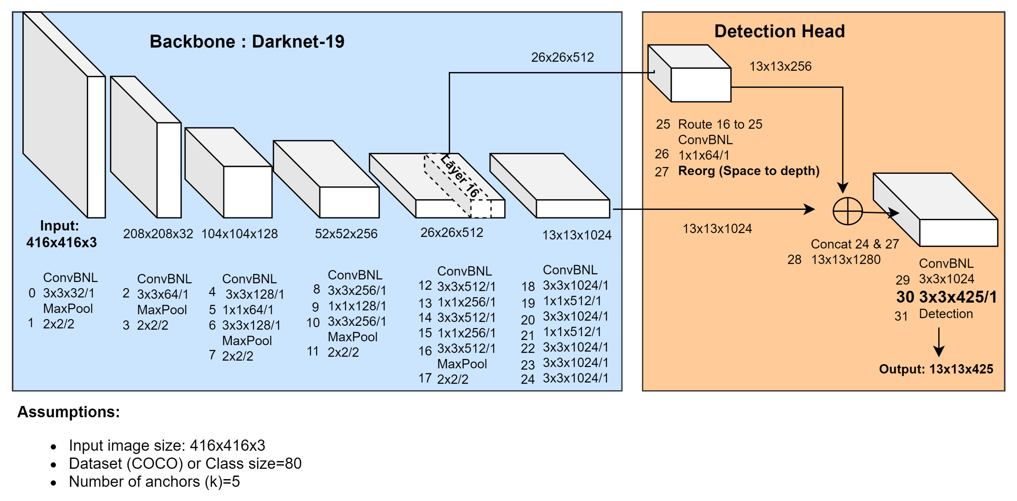
Figure 1. YOLOv2 object detection model layers and their corresponding tensor shapes. ConvBNL stands for convolution followed by batch normalization and Leaky Relu activation layers. Numbers 0–31 show the YOLOv2 layers. For a detailed understanding of each layer’s parameter size, refer to Table 1.
Electronics 11 01827 g001
Figure 2. Feature maps and weight tensors representation of a particular convolution layer. Although not indicated in the figure, usually convolution layers have also learned bias (B) parameters of size equal to the number of output channels, that is N o f . That is one bias value per output channel.
Electronics 11 01827 g002
Figure 3. Space-to-Depth.
Electronics 11 01827 g003
Figure 4. Depth-to-Space.
Electronics 11 01827 g004
Figure 5. Overall architecture of the proposed HW/SW co-design of the inference acceleration system.
Electronics 11 01827 g005
Figure 6. Convolution layer with loop tiling of the input, output and weight ‘pixels’ or ‘feature maps’.
Electronics 11 01827 g006
Figure 7. Illustration of double-buffering sequencing.
Electronics 11 01827 g007
Figure 8. Weight 4D–3D reorganization. The colors are only to show a sample of the corresponding pixels’ positions before and after the reorganization of the weight tensor.
Electronics 11 01827 g008
Figure 9. Convolution processing element and its working procedure.
Electronics 11 01827 g009
Figure 10. Convolution processor architecture.
Electronics 11 01827 g010
Figure 11. Max-pool processor.
Electronics 11 01827 g011
Figure 12. Per-layer latency of YOLOv2 inference on ZYNQ 7020 and ZCU102.
Electronics 11 01827 g012
Figure 13. Sample YOLOv2 inference output of our hardware accelerator.
Electronics 11 01827 g013
Table 1. YOLOv2 layers and their input and output sizes presented in detail.
LayerLayer TypeFiltersSize/StrideInput SizeOutput Size
Darknet-19 Backbone0ConvBNL32 3 × 3 / 1 416 × 416 × 3 416 × 416 × 32
1Max Pool 2 × 2 / 2 416 × 416 × 32 208 × 208 × 32
2ConvBNL64 3 × 3 / 1 208 × 208 × 32 208 × 208 × 64
3Max Pool 2 × 2 / 2 208 × 208 × 64 104 × 104 × 64
4ConvBNL128 3 × 3 / 1 104 × 104 × 64 104 × 104 × 128
5ConvBNL64 1 × 1 / 1 104 × 104 × 128 104 × 104 × 64
6ConvBNL128 3 × 3 / 1 104 × 104 × 64 104 × 104 × 128
7Max Pool 2 × 2 / 2 104 × 104 × 128 52 × 52 × 128
8ConvBNL256 3 × 3 / 1 52 × 52 × 128 52 × 52 × 256
9ConvBNL128 1 × 1 / 1 52 × 52 × 256 52 × 52 × 128
10ConvBNL256 3 × 3 / 1 52 × 52 × 128 52 × 52 × 256
11Max Pool 2 × 2 / 2 52 × 52 × 256 26 × 26 × 256
12ConvBNL512 3 × 3 / 1 26 × 26 × 256 26 × 26 × 512
13ConvBNL256 1 × 1 / 1 26 × 26 × 512 26 × 26 × 256
14ConvBNL512 3 × 3 / 1 26 × 26 × 256 26 × 26 × 512
15ConvBNL256 1 × 1 / 1 26 × 26 × 512 26 × 26 × 256
16ConvBNL512 3 × 3 / 1 26 × 26 × 256 26 × 26 × 512
17Max Pool 2 × 2 / 2 26 × 26 × 512 13 × 13 × 512
18ConvBNL1024 3 × 3 / 1 13 × 13 × 512 13 × 13 × 1024
19ConvBNL512 1 × 1 / 1 13 × 13 × 1024 13 × 13 × 512
20ConvBNL1024 3 × 3 / 1 13 × 13 × 512 13 × 13 × 1024
21ConvBNL512 1 × 1 / 1 13 × 13 × 1024 13 × 13 × 512
22ConvBNL1024 3 × 3 / 1 13 × 13 × 512 13 × 13 × 1024
23ConvBNL1024 3 × 3 / 1 13 × 13 × 1024 13 × 13 × 1024
Detection Head24ConvBNL1024 3 × 3 / 1 13 × 13 × 1024 13 × 13 × 1024
25Route 16 26 × 26 × 512
26ConvBNL64 1 × 1 / 1 26 × 26 × 512 26 × 26 × 64
27Reorg /2 26 × 26 × 64 13 × 13 × 256
28Concat 24 and 27 13 × 13 × 1280
29ConvBNL1024 1 × 1 / 1 13 × 13 × 1280 13 × 13 × 1024
30ConvBNL425 1 × 1 / 1 13 × 13 × 1024 13 × 13 × 425
31Detection-head (output post-processing)
Table 2. Loop tile sizes and memory read–write access iterations to or from the tile buffers.
TensorsOriginal ShapeTile Sizes (Shapes)Number of External Memory Access (Either to Read from or Write to DDR Memory)
IFM N i f × N i x × N i y T i f × T i x × T i y N o f T o f × N i f T i f × N o x T o x × N o y T o y
OFM N o f × N o x × N o y T o f × T o x × T o y N o f T o f × N o x T o x × N o y T o y
Weights N o f × N i f × N k x × N k y T o f × T i f × T k x × T k y N o f T o f × N i f T i f
Biases N o f T o f N o f T o f
Table 3. Available resources onboard ZYNQ-7020 and ZCU102.
Boards          Z-7020CGL484-1          ZCU102-XCZU9EG-2FFVB1156E
Flip flops (FF)106,400548,160
LUT53,200274,080
BRAM_18Kb2801824
DSP2202520
Table 4. Design parameter choices and performance measures.
Boards          ZYNQ 7020          ZCU102
Tile sizes T o f 3264
T i f 44
T o x 2652
T o y 2652
T i x 52104
T i y 52104
Resource utilizationFF22,239 (20.9%)34,076 (6%)
LUT28,333 (53.2%)97,971 (35%)
BRAM (18 Kb)170 (60.7%)1008 (55%)
DSP180 (81.8%)291 (11%)
Clock (MHz)150300
GOP44.3644.96
GOPS51.06184.06
Power (Watt)2.785.376
Table 5. Comparison of our implementation against other prior works using several metrics.
 [30] [31] [32] [33] [23]This WorkThis Work
DeviceVirtex-7 VC707ZCU102ZedboardIntel Arria 10Intel Stratix 10ZYNQ-7020ZCU102
ModelsSim-YOLOv2YOLOv2YOLOv3 tinyYOLOv2SSD300YOLOv2YOLOv2
Design toolOpenCLVivado HLSVivado HLSOpenCLRTLVitis HLSVitis HLS
Design schemeHWHW/SWHW/SWHW/SWHW/SWHW/SWHW/SW
Precision (bits)1–616168–168–161616
Frequency (MHz)200300100200300150300
FF Utilization115 K (18.9%)90,58946.7 K523.7 K-22.2 K (20.9%)34,076 (6%)
LUT Utilization155.2 K (51.1%)9513625.9 K360 K532 K28.3 K (53.2%)97,971 (35%)
DSP Utilization272 (9.7%)6091604104363180 (81.8%)291(11%)
BRAM(18Kb) utilizations1144 (55.5%)4911851366 *3844 *170 (60.7 %)1008 (55%)
Throughput (GOP/S)1877102.5464.7740217851.06184.06
Power18.2911.83.3627.21002.785.376
Latency (ms)-288532-29.11868244
Accuracy (mAP)64.16--73.676.9476.2176.21
Input image size 416 × 416 416 × 416 - 416 × 416 300 × 300 416 × 416 416 × 416
* Intel FPGA with BRAM 20 Kb.
Publisher’s Note: MDPI stays neutral with regard to jurisdictional claims in published maps and institutional affiliations.

