Abstract
Ensuring that a vehicle can obtain its real location in a high-precision prebuilt map is one of the most important tasks of the Autonomous Internet of Vehicles (AIoV). In this work, we show that the resampling of the particle filter (PF) algorithm is optimized by using the prior information of particles that shift real localizations to improve vehicle localization accuracy without changing the existing PF process, i.e., the particle shift filter (PSF). The number of particles is critical to their convergence efficiency. We perform quantitative and qualitative analyses of how to improve particle localization accuracy while ensuring timeliness, without increasing the number of particles. Moreover, the cumulative error of the particles increases with time, and the localization accuracy and robustness decrease. Our findings show that the initial particle density is 159 particles/m, and the cumulative variance of the PSF particles is improved by 27%, 29%, and 82% at the x-, y-, and z-axes, respectively, under the same conditions as the PF algorithm, while the calculation time only increases by 10.6%. Moreover, the cumulative mean error is reduced by 0.74 m, 0.88 m, and 0.68 m at the x-, y-, and z-axes, respectively, indicating that the localization error of the PSF changes less with time. All experiments were performed using open-source software and datasets.
1. Introduction
Localization technology plays an important role in the Autonomous Internet of Vehicles (AIoV). In general, precise vehicle localization can provide vehicles with centimeter-level lane departure warnings, location-based services, and more [1]. Traditional localization technologies such as global navigation satellite system (GNSS) localization and real-time kinematic (RTK) localization are relatively mature, and are able to achieve highly accurate localization. However, their performance will be influenced when satellite signals are blocked by tunnels, houses, and forests [2,3]. At the same time, the strict driving safety requirements of the AIoV entail higher requirements for localization accuracy, real-time computing, and environmental adaptability. Furthermore, the energy system of the AIoV is mainly powered by batteries, and vehicle localization should be based on the principle of not adding additional sensors, so as to reduce the energy consumption of in-vehicle equipment [4].
To overcome the above challenges, many researchers have collected data on traffic infrastructure, generally observed in real driving environments, for vehicle localization. High-precision map localization is achieved by matching maps with built-in-vehicle sensor data. The sensors that is mainly used for the high-precision map localization are 3D-LiDAR. The measurements obtained from 3D-LiDAR are matched with a high-precision map to help in vehicle localization. Therefore, high-precision map localization algorithms based on 3D-LiDAR have been widely studied. In the localization process of a high-precision map based on point clouds, real-time observation data from 3D-LiDAR are not the same as map data due to the non-real-time character of a map and the noise of the sensors, which causes a local optimum or a localization of non-convergence. This will affect the accuracy of point cloud localization algorithms matched with maps.
At present, point cloud localization technologies mainly include map-matching algorithms based on an iterative closest point (ICP) algorithm combined with normal distribution transform (NDT) and statistical algorithms such as PF, the unscented Kalman filter (UKF), and the histogram filter (HF) based on Bayesian filtering. These two kinds of algorithms usually use the matching degree of observation points and map data to locate vehicles. When the ICP algorithm combined with NDT is used for locating objects, initial pose information of the objects is needed to narrow the scope of localization, and the observation data and the map data will then be iterated and matched. If the distance error between the observation data and the map data becomes smaller after iterations and meets a certain threshold, the pose of the observation data after matching is the localization result. In [5], the NDT algorithm was used to achieve rough localization, and the ICP algorithm was then used for map matching with higher accuracy to finish the localization. A method of building a map by extracting the vertical features of a point cloud map was proposed in [6]. This method uses the ICP algorithm to match angle features extracted in real time with the vertical angle features of the map to achieve localization. Yoneda et al. [7] extracted map features through the feature quantity of scanned data based on cluster distribution, and used the ICP algorithm for localization. A method of matching and localization by extracting rod-shaped objects features is proposed in [8]. Additionally, there are also map matching algorithms based on features such as height [9] and road edge [10,11,12,13]. However, those map-based matching algorithms usually need to extract the point cloud features, and there are problems, such as the high sensitivity of the initial localization value to noise, the time-consuming process of feature extraction and registration, and a poor localization accuracy. Therefore, it is hard to meet the AIoV requirements of high-precision real-time localization.
The statistical method is usually divided into two processes: localization prediction and update. In the localization prediction stage, the observation data are predicted through an initial pose and system motion model. Subsequently, the matching degree between the predicted observation data and the map is calculated to indicate its uncertainty. The higher the mismatch degree is, the greater the uncertainty will be. Secondly, in the localization update phase, the mean and variance of pose are updated by using the difference between the real observation data and the predicted observation data as well as the matching degree as the localization output. In [14,15], the inconsistency between high-precision point cloud map data and point cloud data collected in real time is expressed by probability. The authors converted the localization process into two steps, including prediction and a prediction update, to obtain a better prediction of the uncertainty of localization. In the prediction stage, the observation data are predicted through the initial pose and the system motion model, and the matching degree between the predicted observation data and the map is then calculated to show its uncertainty. The higher the mismatch degree is, the greater the uncertainty will be. In the stage of the prediction update, the differential and matching degree between the observation data collected in real time and the predicted observation data is used to update the mean value and variance of the pose, and the updated mean value and variance are then used as the localization output. Therefore, due to its excellent anti-noise ability and robustness for various scenes, the localization algorithm based on filters has been widely studied in autonomous driving localization [16,17]. Castorena et al. [16] built a ground reflectivity map based on a point cloud and implemented localization by an extended Kalman filter (EKF) localization algorithm. To achieve better precision and comparable stability in the localization, Lin et al. [17] proposed a particle-aided unscented Kalman filter (PAUKF) algorithm. They updated position measurement information based on an onboard sensor and a high definition (HD) map. In [18], they enhanced the weights of the particles by adding Kalman-filtered Global Navigation Satellite System (GNSS) information to improve autonomous vehicle localization. Feng et al. [19] used a UKF-based SLAM algorithm to estimate a robot pose and feature map. Jia et al. [20] used the Point-to-Line Iterative Closest Point (PL-ICP) to register the laser scan data of two adjacent frames and combined this with the Rao-Blackwillised Particle Filter (RBPF) for localization. For maximum performance, the localization algorithm based on a KF usually needs to be in a linear Gaussian system [21], while a filtering localization algorithm and a PF algorithm based on an HF algorithm can adapt to any nonlinear non-Gaussian system and have higher localization accuracy. Compared with the KF algorithm and the HF algorithm, the nonlinear change capability of the PF algorithm makes it able to adapt to both linear and nonlinear systems without a specific posterior probability density function. Through rod-shaped objects in a point cloud map and a reflectivity map, Blanco et al. [22] designed a localization algorithm based on a PF algorithm through a pre-built high-precision map. This algorithm updated particles according to the distance between each scanning point and the map until convergence, and localization accuracy was significantly improved. An improved particle filter algorithm based on an optimized iterative Kalman filter is proposed in [23]. The algorithm used fewer particles for sampling, which reduced the amount of computation and improved the real-time performance of the algorithm. In [24], a map sharing strategy is proposed; in this strategy, each particle has only a small map of the surrounding environment. However, due to the inconsistency between the high-precision point cloud map and the point cloud data collected in real time, as well as the randomness of the particle, the calculated value of the particle weight does not accurately reflect the correctness of its localization. Thus, autonomous driving point cloud localization technology based on a PF algorithm often shows deficiencies, such as slow convergence and particle degradation, which seriously reduce localization accuracy. In order to solve the problems of local optimization caused by the randomness of particles in the PF algorithm, a localization algorithm framework based on prior information fusion is proposed in this paper. The framework utilizes the prior information between the observation data and the map to optimize the intermediate parameters of the algorithm, so as to make up for the deficiency of the existing localization algorithm frameworks. According to the proposed framework, an improved PF localization algorithm based on particle shift is proposed to improve the localization accuracy. The contributions of this paper are summarized as follows:
- This paper proposes a localization system framework based on prior information fusion. The framework considers prior information where the observation data is most similar to the map data of the real location of the vehicle in the point cloud map, and constructs its relationship model with the state transition particle set of the localization algorithm, which reduces the influence of occlusion and dynamic noise on the positioning accuracy.
- To perfect the framework design, a particle shift filter localization algorithm is proposed. We calculate the similarity between the transferred point cloud and the map point cloud. We then resample the particles based on the similarity, and the particles represented by the point cloud with higher similarity can be selected as the final localization particles.
The rest of this paper is structured as follows. The localization algorithm framework based on prior information fusion and the improved PF algorithm based on particle shift are presented in Section 2. Section 3 discusses the verification process in the experiments and analyzes the errors. Finally, the conclusion is provided in Section 4.
2. Problem Statement and System Framework
2.1. Problem Statement
The current popular point cloud localization system framework usually takes the observation data, the point cloud map, and the initial localization data as input data. Subsequently, statistical algorithms such as PF filtering can be performed in the localization module, and localization estimation is carried out according to the matching degree, which is determined by the sum of corresponding point distances between the observation data and the point cloud map. The smaller the sum of the distance is, the higher the matching degree will be. However, in a real 3D environment, point cloud localization algorithms usually judge the accuracy of the localization through the distance error between the point cloud due to the complexity of automatic driving environments and the randomness of the point cloud in the map. The distance error, as a scalar, can measure the matching degree of two point clouds to a certain extent but cannot reflect their structural differences due to initial localization errors and sensor errors, causing poor localization precision. To improve the precision of localization, this paper proposes a localization system framework based on prior information fusion. The framework considers the prior information where the observation data is most similar to the map data of the real vehicle location in the point cloud map, and constructs its relationship model with the localization algorithm. Subsequently, the prior information is fused into the localization algorithm framework. The system framework is shown in Figure 1.
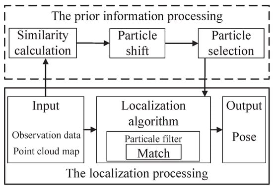
Figure 1.
System framework.
The framework of the point cloud localization system based on prior information fusion proposed in this paper includes two parts: localization processing and prior information processing. The localization processing includes data input, localization, and output, which is consistent with the current popular point cloud location processing framework. The prior information processing includes a similarity calculations, particle shift, particle selection, and fusion localization. First, the similarity calculation extracts the similarity between the observation point cloud and the map from the input data. The particle shift is used to find the particles close to the real localization in the particle update stage. Subsequently, particle selection is carried out based on the particle shift, such that the particles used for positioning converge in the direction of greater similarity. Fusion localization is achieved by particle resampling.
In the positioning state prediction stage, the particle filter needs to sample m particles to form a particle pose set and then predict and transfer the state of particles to obtain a new particle set. Subsequently, the weight of the particle is calculated, and the particle set is resampled. The resampled particle set determines the final positioning output of the particle filter algorithm. Therefore, if we can optimize the particle set after the transfer and improve the convergence and accuracy of the particle set, the positioning output will be improved. Therefore, the basic idea of the PSF is to calculate the similarity between the transferred point cloud and the map point cloud. The higher the similarity is, the greater the particle weight is. We then resample the particles based on the similarity, and the particles represented by the point cloud with higher similarity can be selected as the final localization particles. This allows particles used for localization to converge in the direction of greater similarity and improves positioning accuracy.
In this paper, the PSF algorithm mainly includes a state transition and observation. Generally, a dynamic system can be represented by the state transition probability (prior probability) and the observation probability . In addition, the reliability (posterior probability) of the state of the current dynamic system is estimated based on the historical observation and the past control vector . According to Bayesian theory, the relationship between prior probability and posterior probability is as follows:
However, due to the influence of obstacles and noise, and since the change trend of the particle set is nonlinear, there are many errors in the calculation of . After particle resampling, in the process of particle renewal, it may cause particle degradation and finally fall into a local optimum. Therefore, we seek to find the relationship between the particles and the true value, recalculate and update the particles to ensure the diversity of the particles, and achieve more accurate localization. Given , the particle set generated by the state transition, and , another particle set generated by calculating the weight and resampled, is the particle weight. The output of localization is as follows:
where represents the accuracy of the PF localization algorithm prediction. The closer its value is to the true value, the smaller the error is, and the higher the localization accuracy is. The variance indicates the degree of the convergence of the particles. The variance and convergence of the particles are inversely proportional. As the variance reduces, the particle-to-particle distance also decreases, and the localization becomes more stable. According to the localization algorithm framework proposed in Figure 1, we seek to design an optimization algorithm for the intermediate parameter of the particle set, which can obtain a smaller variance.
We denote each particle as a six-vector particle, with parameters containing three-dimensional coordinates, the vehicle heading angle, the pitch angle, and the roll angle, recorded as . In order to calculate the particle weight, it is necessary to transfer the observation point cloud obtained by the LiDAR on the vehicle to gain the observation point cloud in global coordinates. The particles can be shifted by
where represents the rotation of the angular state of the vehicle, and represents the translation of the coordinates of the particles. The point cloud corresponding to the particle is also transformed by the same rotation and translation to obtain the observation point cloud in global coordinates. We then calculate the Euclidean distance between the transferred point cloud and the map point cloud to judge the similarity between the two. The sum of the distance between the observation point cloud and the map point cloud reduces, the similarity increases correspondingly, and the weight also increases. Finally, the point cloud with higher similarity is screened out through resampling it as the final localization particle.
In order to optimize the particle set after the state transition, the convergence of the particle set after weight calculation and particle resampling is higher; thus, localization accuracy is improved.
2.2. Similarity Calculation and Particle Shift
The particle shift process matches observation data to the map in the particle update stage to make particles closer to the real localization. This is based on the following facts.
- (1)
- Each particle is regarded as one possible localization point. The particle weight indicates the similarity between the observation point cloud and the data around the localization point. As a scalar, Euclidean distance is used in the convergence process to measure the similarity between the particle and its true value.
- (2)
- For the randomness of particles and the complexity of the traffic environment, the localization indicated by the particles with a high similarity is not true, but the particles near the true value will be close to the true value.
In order to calculate the particle shift, this paper assumes that the state space is continuous and that the real localization point is included in this space. Ideally, as the localization accuracy increases, the similarity between the particles and the real state increases, so the point-to-point corresponding distances between the observation particle and the map are smaller. In this paper, the variable represents the similarity, which is the average inverse of the sum of the distance between the observation point cloud and the map point cloud.
where is a point in the observation point cloud, and denotes the nearest point to . After the particles converge, the particles are transformed, and the value of the particles increases, such that the particles approach the true value. In order to calculate this transformation, it needs to be converted into a least squares problem.
The observation point cloud is represented by the set , and the set of the closest points corresponding to in the map is represented by . The centroid of the set is represented by .
The centroid of the set is represented by .
We define a transformation matrix as , where is a rotation matrix, and is a translation matrix. and are obtained by minimizing the opposite of similarity . The formula is described as
We then obtain a corresponding solution through singular value decomposition, i.e., a rotation transformation matrix. A shifting particle is chosen with the value increased after transformation.
2.3. Particle Selection
After the particles shift, the point cloud with its closest observation point changes. The similarity between the shifting particles and the true value may decrease. In order to solve the problem that particles may fall into local optimization after shifting, this paper introduces a simulated annealing algorithm to select the shifted particles, optimizing particle shift while maintaining particle diversity.
The flow chart of the particle shift selection algorithm based on the simulated annealing algorithm is shown in Figure 2. The observation point cloud carried by the shifted particles is represented by the point set , and the closest point set between the point set and the map is represented by . The similarity after the particle shift is represented by .
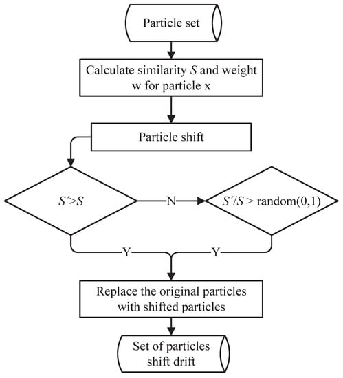
Figure 2.
The particle selection method.
If , the shifted particle is valid, and it will be added to the particle set . If , we compare the value between and the probability p. If the , we select this particle shift; otherwise, no particle shift is required, and the particle remains unchanged. Through the above selection algorithm, the PSF algorithm can be further prevented from falling into the local optimization, and the problem of particle degradation can be alleviated. The particle selection algorithm can be described in Algorithm 1. is the particle set obtained through prediction in the PSF algorithm. is the weight calculated by similarity. represents the point cloud collected by the vehicle in real time. represents the high-precision point cloud image. represents the particle shift calculation algorithm based on Section 2.2. The output is the particle set changed by the particle shift algorithm.
| Algorithm 1 Particle Selection. |
| Input: Output: 1: 2: fordo 3: 4: 5: if then 6: and 7: else 8: if then 9: and 10: else 11: do nothing 12: end if 13: end if 14: end for 15: return ; 16: |
2.4. PSF Based on Prior Information
There are four steps in the PSF algorithm: sampling, particle shift, weighting, and resampling. The algorithm makes the particles close to the real value with the shift of particles in order to obtain a higher localization accuracy. Figure 3 shows the PSF algorithm for localization combined with the high-precision point cloud map and the real-time observation data. The steps of the PSF localization algorithm are as follows:
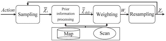
Figure 3.
The PSF localization algorithm.
- (1)
- In the initialization stage, the original particle pose is obtained by uniform sampling in the possible localization area, and its weight is the same.
- (2)
- In the state prediction stage of localization, the data is used to transfer the state of the particles to obtain the particle pose after the transfer. Moreover, because the particle set is discrete in practical applications, it is usually possible to directly use the particles after the state transition to form a particle set without reducing the number of particles, which is expressed as .
- (3)
- Since the particle set after the state transition is mixed with a high amount of noise, the particle aggregation becomes divergent. and measurement data are used in the particle shift algorithm to shift the particles before the particles calculate and update the weights. The updated particle set is more convergent to prevent particle degradation. The obtained optimized particle set after the shift is denoted as .
- (4)
- The particle weight of the shift particle set is calculated.
- (5)
- In the state update stage of localization, the weights of the shifted particles are normalized, and the particles are then resampled according to the weights. A new particle set is reconstructed.
- (6)
- The cumulative mean and the variance of the output particle set are used as the location estimation results. Starting again from Step (1), is then used as the the original set of particle poses in the next iteration. We assume that the localization result is obtained at time and that , , and are the mean values of the localization. Taking the x-axis as an example, the localization error is as followswhere represents the localization error on the x-axis at time . is the mean of the coordinates of n particles on the x-axis at time . i.e., . represents the true value of the positioning on the x-axis at the current moment.
The cumulative mean error is obtained by adding the localization error values , , , at all times. The cumulative mean error means the cumulative degree of the localization error. The smaller the cumulative localization error is, the higher the localization stability of the algorithm is. The formulation for the cumulative mean error is given by
The cumulative variance represents the convergence performance of the particles in the particle filter algorithm. The smaller the variance is, the closer the particle is to the real localization, which means that the particle filter has a higher convergence performance. The cumulative variance of the coordinates of n particles on the x-axis at time is defined as
where .
3. Experimental Results
In order to test the improved PF localization algorithm, this paper adopts the KITTI dataset, which is used internationally as simulation data. The dataset S03 corresponds to a suburban area, S05 corresponds to a residential area, and S07 corresponds to a town. These three scenarios are used as test data. Meanwhile, Gaussian noise is added to the ground truth of the three datasets to simulate the localization errors of the GNSS in reality. The localization area is a space with a radius of 0.5 m. The computer used for the experiment has 8 G of RAM, a Core (TM) i5-4200m CPU, a 2.5 GHz main frequency, a Windows 10 operating system, and the open resource library PCL1.72 for point cloud processing.
3.1. Qualitative Analysis
According to the proposed particle shift algorithm, the high-precision point cloud map was first input and used as a reference for localization. All points in the point cloud map were then constructed into a fast index map by KD-Tree, which was used for searching the nearest points and calculating during the localization process. Based on the particle shift algorithm, the value of the particle shift was found for higher particle convergence and more accurate localization. The effect of particle shift is shown in Figure 4. The red and blue points in the figure both represent particles, and the green points represent the raw point cloud. Figure 4a is a visualization of particles after particle resampling based on the particle filter localization algorithm, and Figure 4b is the visualization of particles after the particle shift algorithm. Comparing the particle set in Figure 4a and the particle set in Figure 4b shows that the shifting particle set is closer in space, which means the degree of convergence of the particles is higher.
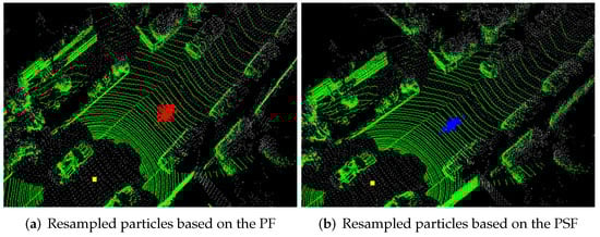
Figure 4.
Comparison with different particle filter algorithm for resampled particles.
3.2. Localization Error Analysis
We used the S07 dataset for testing. The initial localization was set as the origin of the axis, and the rotation angle of each axis of the vehicle was 0. Uniform sampling was conducted in the x and y planes of a circular region with a center radius of 1 m, where the initial localization is the center. On the z-axis, however, the 3D-LiDAR was taken as the center, and the region floating up and down 0.2 m was uniformly sampled n times. On the three axes of yaw, pitch, and roll, Gaussian noise with a mean of 0 rad and a variance of 1 rad was added to each, to sample them n times. Finally, the value after sampling was taken as the initial value of the particles, and the number of samples was the number of particles. The number of samples in the experiment was set to 200. In the process of localization, Gaussian noise was added to the change in the vehicle pose at each moment to simulate the control input obtained from the vehicle control module. Gaussian noise with a mean of 0 m and a variance of 0.6 m was added to the control incremental coordinates of the directions x, y and z, and Gaussian noise with a mean of 0 rad and a variance of 0.1 rad was added to the three rotation angles of yaw, pitch, and roll. These pose changes with noises were used as the control state quantity in the PF for particle prediction. Figure 5 shows the output results of the comparison in the localization on the x, y, and z axes and the heading angle yaw based on the PF algorithm and the PSF algorithm proposed in this paper. x corresponds to different times, and y represents the error values of the directions of each axis and the heading angles represented by the localization output and ground truth of the two algorithms in each axis. In the x-, y-, and z-axes, the error between the PSF is closer to 0 than that between the PF and the true value. In the heading angles, the error of the localization result of the PSF algorithm is also smaller than that of the PF algorithm.
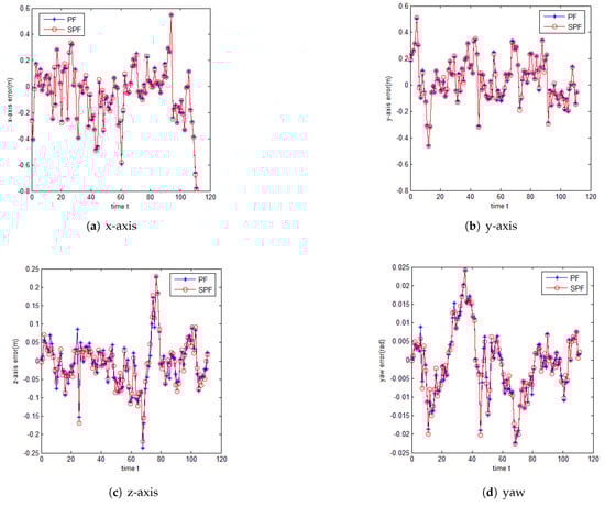
Figure 5.
Localization error.
Figure 6 shows the cumulative comparison of localization errors between the PSF algorithm and the ground truth and between the PF algorithm and the ground truth on the x-, y-, and z-axes in the 100 localization outputs of this experiment. Through the comparison, it was found that, in the directions of each coordinate axis, the cumulative localization error of the PSF algorithm was lower than that of the PF algorithm. In the x-axis, the cumulative error was reduced by 0.74 m, and the cumulative accuracy was improved by 11%. In the y-axis, the cumulative error was reduced by 0.88 m, and the cumulative accuracy was improved by 10%. In the z-axis, the cumulative error was reduced by 0.68 m, and the cumulative accuracy was improved by 14%. The experimental results achieve the purpose of improving the localization accuracy.
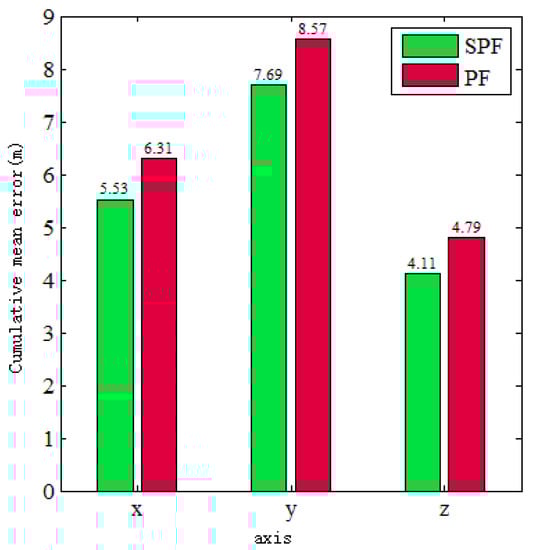
Figure 6.
Cumulative mean error.
Figure 7 illustrates a comparison experiment of 100 localization outputs on the x-, y-, and z-axes between the localization cumulative variances of the PSF algorithm and the ground truth and between those of PF algorithm and the ground truth. It was found that the localization cumulative variance of the particle set after shifting was less than the localization variance of the particle set without shifting. The cumulative localization variances in the x-, y-, and z-axes were reduced by 3.13 m, 3.14 m, and 1.81 m. Meanwhile, the cumulative accuracy in the x-, y-, and z-axes was improved by 27%, 29%, and 82%. This shows that the differences in particles in the particle set after shifting were smaller on each axis. A large number of ground point clouds can provide a reliable matching reference in the z-axis, so the variance of particles shifting in the z-axis was smaller, and the degree of convergence was significantly higher than in the x- and y-axes.
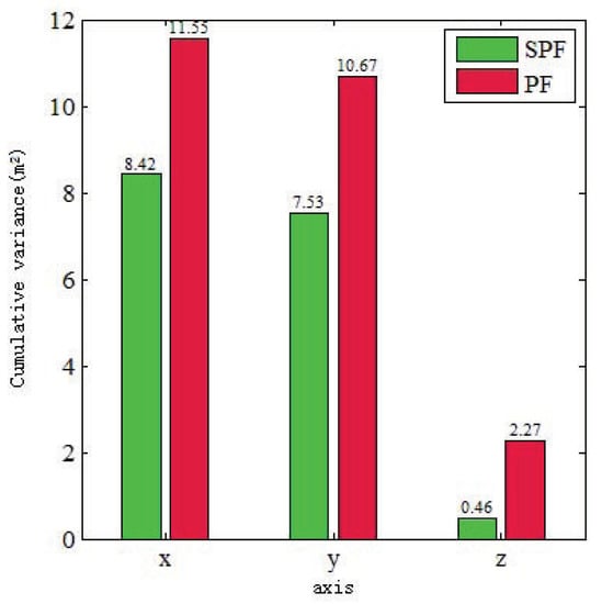
Figure 7.
Cumulative variance comparison.
Figure 8a shows the trajectory of the localization algorithm obtained in this experiment, in which “+-” represents the real vehicle trajectory, “*-” represents the localization trajectory obtained by the PF algorithm, and “o-” refers to the trajectory obtained by the PSF algorithm. The localization trajectories obtained by the PF algorithm and the PSF algorithm were almost identical, and the deviation from the real vehicle trajectory was only 0.4 m. However, the local trajectory map in Figure 8b shows that the trajectory obtained by the PSF algorithm was closer to the ground truth, indicating that its localization accuracy was higher.
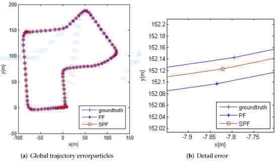
Figure 8.
Localization trajectory.
Finally, we compared the localization time of the above two algorithms with different numbers of particles under the same experimental environmen shown in Figure 9.
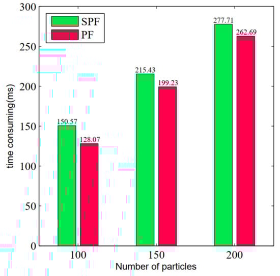
Figure 9.
Time-consumption comparison with different numbers of particles.
Although the calculation time for particle shift of the PSF algorithm is about 20 ms longer than that of the PF algorithm, the time used to calculate particle shift is much less than that of the PF algorithm itself. The experimental result shows that introducing the particle shift algorithm into the PF algorithm not only does not significantly increase the time of the particle-filter-based localization algorithm, but also improves its accuracy and convergence.
4. Conclusions
This paper proposes a PSF localization algorithm framework based on prior information fusion. First, the algorithm computes the prior information similar to the raw point cloud data and the map data of the actual localization of the vehicle. Second, in the particle update stage, the particle shift process matches the observation data to the map. Next, the resampling of the PF algorithm is optimized by using the prior information to improve vehicle localization accuracy. However, the PSF localization algorithm relies on the precise location data of GPS and IMU in the initial stage of localization, so the application prospect of our algorithm is weaker without the assistance of GPS and IMU. In the future, we plan to design an algorithm that enables map-aided vehicle localization without any additional assistance from GPS or IMU.
Author Contributions
Conceptualization, Q.C. and X.L.; methodology and software, X.T. and D.W.; validation, Z.S. and D.W.; writing—original draft preparation and editing, Q.C. and X.T. All authors have read and agreed to the published version of the manuscript.
Funding
This work was supported by grants from the Guangxi Natural Science Foundation (2019GXNSFFA245007), the Key Science and Technology Project of Guangxi (AB21196032), and the National Natural Science Foundation of China (61762030).
Conflicts of Interest
The authors declare no conflict of interest.
References
- Jiang, M.; Wang, H.; Zhang, W.Y.; Qin, H.; Sun, X. Location-based data access control scheme for Internet of Vehicles. Comput. Electr. Eng. 2020, 86, 106716–106725. [Google Scholar] [CrossRef]
- Kim, K.W.; Im, J.H.; Jee, G.I. Tunnel Facility Based Vehicle Localization in Highway Tunnel Using 3D LIDAR. IEEE Trans. Intell. Transp. Syst. 2022, 1–9. [Google Scholar] [CrossRef]
- Ahmad, T.; Li, X.J.; Seet, B.C. Parametric Loop Division for 3D Localization in Wireless Sensor Networks. Sensors 2017, 17, 1697. [Google Scholar] [CrossRef] [PubMed] [Green Version]
- Manfren, M.; Nastasi, B.; Groppi, D.; Garcia, D.A. Open data and energy analytics—An analysis of essential information for energy system planning, design and operation. Energy 2020, 213, 118803–118832. [Google Scholar] [CrossRef]
- Wang, Q.S.; Zhang, J.; Liu, Y.S.; Zhang, X.C. Point Cloud Registration Algorithm Based on Combination of NDT and ICP. Comput. Electron. Agric. 2020, 56, 88–95. [Google Scholar]
- Im, J.H.; Im, S.H.; Jee, J.I. Vertical Corner Feature Based Precise Vehicle Localization Using 3D LIDAR in Urban Area. Sensors 2016, 16, 1268. [Google Scholar] [CrossRef] [PubMed] [Green Version]
- Yoneda, K.; Tehrani, H.; Ogawa, T.; Hukuyama, N.; Mita, S. LiDAR scan feature for localization with highly precise 3-D map. In Proceedings of the IEEE Intelligent Vehicles Symposium Proceedings, Dearborn, MI, USA, 8–11 June 2014; pp. 1345–1350. [Google Scholar]
- Li, L.; Yang, M.; Weng, L.; Wang, C. Robust Localization for Intelligent Vehicles Based on Pole-Like Features Using the Point Cloud. IEEE Trans. Autom. Sci. Eng. 2021, 19, 1095–1108. [Google Scholar] [CrossRef]
- Wolcott, R.W.; Eustice, R.M. Robust LIDAR localization using multiresolution Gaussian mixture maps for autonomous driving. Int. J. Robot. Res. 2017, 36, 282–319. [Google Scholar] [CrossRef]
- Schlichting, A.; Brenner, C. Vehicle localization by lidar point correlation improved by change detection. Int. Arch. Photogramm. Remote Sens. Spat. Inf. Sci. 2016, 41, 703. [Google Scholar] [CrossRef] [Green Version]
- Zhuang, J.C.; Qin, B.X.; Bandyopadhyay, T.; Ang, M.H.; Frazzoli, E.; Rus, D. Synthetic 2D LIDAR for precise vehicle localization in 3D urban environment. In Proceedings of the IEEE International Conference on Robotics and Automation, Karlsruhe, Germany, 6–10 May 2013; pp. 1554–1559. [Google Scholar]
- Qin, B.X.; Zhuang, J.C.; Bandyopadhyay, T.; Ang, M.H.; Frazzoli, E.; Rus, D. Curb-intersection feature based Monte Carlo Localization on urban roads. In Proceedings of the IEEE International Conference on Robotics and Automation, Saint Paul, MN, USA, 14–18 May 2012; pp. 2640–2646. [Google Scholar]
- Sun, P.P.; Zhao, X.M.; Xu, Z.G.; Wang, R.M.; Hai, G.M. A 3D LiDAR Data-Based Dedicated Road Boundary Detection Algorithm for Autonomous Vehicles. IEEE Access 2019, 7, 29623–29638. [Google Scholar] [CrossRef]
- Ding, W.; Hou, S.; Gao, H.; Song, S. Lidar inertial odometry aided robust lidar localization system in changing city scenes. IEEE Int. Conf. Robot. Autom. 2019, 39, 4322–4328. [Google Scholar]
- Wang, R.D.; Li, H.; Zhao, K.; Xu, Y.C. Robust Localization Based on Kernel Density Estimation in Dynamic Diverse City Scenes Using Lidar. Acta Opt. Sin. 2019, 39, 0528003–0528013. [Google Scholar] [CrossRef]
- Castorena, J.; Agarwal, S. Ground-Edge-Based LIDAR Localization Without a Reflectivity Calibration for Autonomous Driving. IEEE Robot. Autom. Lett. 2018, 3, 344–351. [Google Scholar] [CrossRef] [Green Version]
- Lin, M.; Yoon, J.W.; Kim, B.W. Self-driving car location estimation based on a particle-aided unscented Kalman filter. Sensors 2020, 20, 2544. [Google Scholar] [CrossRef] [PubMed]
- Demiguel, M.A.; Garca, F.; Armingol, J.M. Improved LiDAR probabilistic localization for autonomous vehicles using GNSS. Sensors 2020, 20, 3145. [Google Scholar] [CrossRef] [PubMed]
- Feng, Y.; Yan, M.T.; Bo, J.; Zheng, L.T. SLAM Based on Double Layer Unscented Kalman Filter. In Proceedings of the International Conference on Robots Intelligent System, Beijing, China, 19–22 April 2019; pp. 663–668. [Google Scholar]
- Jia, D.P.; Duan, G.X.; Wang, N.; Zhou, Z.G.; Zhong, Z.Y.; Lei, H. Simultaneous Localization and Mapping based on Lidar. In Proceedings of the Chinese Control and Decision Conference, Nanchang, China, 3–5 June 2019; pp. 5528–5532. [Google Scholar]
- Chen, Q.M.; Dong, C.Y.; Mu, Y.Z.; Li, B.C.; Fan, Z.Q.; Wang, Q.L. An Improved Particle Filter SLAM Algorithm for AGVs. In Proceedings of the International Conference on Control Science and Systems Engineering, Beijing, China, 17–19 July 2020; pp. 27–31. [Google Scholar]
- Blanco-Claraco, J.L.; Jose, L.; Mañas-Alvarez, F.; Torres-Morenomo, J.L.; Rodriguez, F.; Gimenez-Fernandez, A. Benchmarking Particle Filter Algorithms for Efficient Velodyne-Based Vehicle Localization. Sensors 2019, 19, 3155. [Google Scholar] [CrossRef] [PubMed] [Green Version]
- Hu, B.S.; Yu, Q.X.; Yu, H.L. Global Vision Localization of Indoor Service Robot Based on Improved Iterative Extended Kalman Particle Filter Algorithm. J. Sens. 2021, 2021, 8819917. [Google Scholar] [CrossRef]
- Jo, H.G.; Cho, H.M.; Jo, S.J.; Kim, E.T. Efficient Grid-Based Rao-Blackwellized Particle Filter SLAM with Interparticle Map Sharing. IEEE/ASME Trans. Mechatron. 2018, 23, 714–724. [Google Scholar] [CrossRef]
Publisher’s Note: MDPI stays neutral with regard to jurisdictional claims in published maps and institutional affiliations. |
© 2022 by the authors. Licensee MDPI, Basel, Switzerland. This article is an open access article distributed under the terms and conditions of the Creative Commons Attribution (CC BY) license (https://creativecommons.org/licenses/by/4.0/).