High-Accuracy 3D Contour Measurement by Using the Quaternion Wavelet Transform Image Denoising Technique

Abstract

In this paper, we propose an image denoising algorithm based on the quaternion wavelet transform (QWT) to address sinusoidal fringe images under strong noise in structured light 3D profilometry. The analysis of a quaternion wavelet shows that the amplitude image of the quaternion wavelet is easily affected by noise. However, the three phase images, which mainly reflect edge and texture information, are randomly and disorderly distributed with respect to noise. The QWT denoising algorithm is suitable for processing sinusoidal fringe images of complex structures in a high-accuracy 3D measurement system. Sinusoidal fringe images are collected and denoised by using the QWT algorithm and classical Gaussian smoothing (GS) denoising algorithm, and GS is used as a reference for the QWT algorithm. The results indicate that the standard deviation is reduced from 0.1448 for raw sinusoidal fringe images to 0.0192, and the signal-to-noise ratio is improved from 4.6213 dB to 13.3463 dB by using the QWT algorithm. The two algorithms have the same denoising effect for a surface with less information. For a surface with rich information, the details of the 3D contour are lost because of the image “blurring” caused by using the GS algorithm, while all edge details of the 3D contour are reconstructed by using the QWT denoising algorithm because of its characteristic of information and noise being separated from the source. For the measured face mask, the error is less than ±0.02 mm. In addition, it takes less than 20 s to run the QWT algorithm to process eight sinusoidal fringe images, which meets the requirements of high-precision measurements.

1. Introduction

With the presence of new requirements in online industrial inspection, intelligent industrial manufacturing [1], reverse engineering [2], cultural relic restoration [3], medical diagnosis [4], and virtual reality, the development of high-resolution and real-time three-dimensional (3D) contour measurement techniques for complex objects has become extremely urgent. Three-dimensional profile measurement methods include the contact type and noncontact type. The disadvantages of the contact 3D profile measurement technique include the degradation of measurement accuracy from local deformation between the measuring head and the measured object; a time-consuming measurement process that is implemented point by point; and surface damage of the measured object from contact stress between the measuring head and the measured object. These disadvantages constrict its application in modern industry. On the contrary, non-contact measurement, obtaining characteristic parameters by means of acoustic, electromagnetic, optical, etc., overcomes many shortcomings of contact measurement. The 3D optical measurement is recognized as the most promising noncontact 3D profile measurement method and has attracted considerable interest because of its advantages of high resolution, non-destructive testing, fast data acquisition, and flexible implementation with a simple hardware configuration. Typical optical noncontact measurement methods include interferometry, time-of-flight, laser scanning, stereo vision, and structured light measurements. Interferometry is more vulnerable to environmental factors, such as vibration, humidity, air pressure, and temperature. The resolution of time-of-flight method, depending on the timing accuracy, which can be improved by increasing the clock frequency, is usually only at the millimeter level [5]. Moreover, for the time-of-flight method, measurements are carried out by point-by-point scanning, so real-time applications cannot be realized. Stereo vision—observing the same object from two viewpoints to obtain a two-dimensional (2D) image of the object from different perspectives, 3D information of the scene being obtained by calculating the position deviation between the image pixels through the trigonometry principle—hardly meets the requirements of a high-precision measurement because of its dependence on the development of computer vision and the measurement accuracy [6]. The principle of the structured light method [7,8,9,10,11] is to project a line or surface structure on the surface of the object to be tested, obtain the image by an image sensor, and then calculate the 3D coordinates of the object by using the trigonometry principle through the system geometry relationship. For a face structured light measurement, some 2D sinusoidal fringe patterns are usually projected on the surface of the object, and the 3D contour is achieved by phase unwrapping. The surface structured light method is the main scheme used to realize real-time 3D profile measurements without the requirement of scanning operations. However, the measurement accuracy of the structured light method not only depends on the accuracy of the fringe phase of the projected grating but is also closely related to the projection environment and the performance of the detector. Although high-density simulated interference fringes can be produced by using Young’s double-hole interference based on the structure of an optical fiber Mach–Zehnder interferometer (MZI) [12] or white light interference, the fringe of the projection is not strictly a sinusoidal distribution, and the stability, phase-shifting accuracy, and background uniformity of the system need to be further improved. Moreover, the signal-to-noise ratio (SNR) of the projected fringe images from interference structures is very low, and serious noise will lead to phase unwrapping errors of the 3D contour. With the rapid development of digital projection technology, 3D profile measurements based on digital fringe projection (DFP) [8,9,11] have aroused increasing interest in recent years because of the advantages of low cost, simple configuration, high accuracy, and high stability. A typical DFP system consists of a digital projector, one or two array image sensors, and a computer. The digital projector actively projects series of special structured patterns on the surface of the object sequentially, while 3D shape information of the measured object can be obtained by phase unwrapping from a series of images detected by the image sensor. The DFP method eliminates phase unwrapping errors caused by nonsinusoidal projection fringes, unreasonable contrast, inaccurate phase shifts, and other factors. The flexible programmability of DFP brings hope for real-time precise 3D contour measurements. However, the correctness of phase unwrapping is not entirely determined by the projection system, and the noise is also the main cause of the phase unwrapping error. The noise can come from image sensors, double-hole interference, a harsh lighting environment, etc. Therefore, image denoising must be carried out before phase unwrapping when the obtained fringe image contains serious noise. In general, the spectrum analysis of image must be performed, and according to the results of the analysis, an appropriate denoising algorithm, such as Gaussian smoothing (GS) filtering, nonlocal means, etc., is selected. GS can effectively eliminate white noise with uniform amplitude, but it will bring a loss of detailed information, such as the edge and texture of the measured object. Nonlocal, meaning a method of smoothing the area around the target pixels according to some similarity, has high definition, but it comes with a high computational complexity and long processing time [13]. Thus, it is the primary goal of image preprocessing for structured light measurements to find a suitable denoising algorithm that meets the following requirements: eliminating all kinds of noise, especially additive noise and speckle noise; reserving the useful information, especially on the edge of the object; and saving time. In this paper, we propose a new image denoising algorithm based on the quaternion wavelet transform (QWT) to process a series of seriously noisy images for structured light measurements and set up a DFP experimental system to demonstrate our image processing scheme. The QWT denoising algorithm can separate information and noise from the source and can remove both Gaussian noise and salt and pepper noise. Moreover, the QWT algorithm can maintain the sinusoidal shape of the fringe and has high time efficiency [14,15,16]. The results of 3D contour reconstruction for the mask indicate that all edge details are accurately displayed and that the small ripple from sinusoidal shape distortion is suppressed. It only takes less than 18 s to process eight pairs of sinusoidal phase modulation images with 2592 × 3872 pixels by using the QWT algorithm. In addition to the application in this paper, other mainstream 3D measurement methods, such as laser scanning with the single-shot raw [17], rotary speckle projector [18], and etc., involving the restoration and reconstruction of edge, texture, and other feature information under bad noise, the signal analysis and noise processing method based on QWT proposed in this paper is also a useful reference.

In this paper, we first proposed the application of the QWT algorithm in 3D imaging, compared with traditional 3D imaging algorithms, such as GS algorithm; in a bad noise environment, the QWT algorithm retains the texture details of the mask, without loss of the mask details, and improves the accuracy of 3D imaging. It also has lower complexity and shorter processing time than the traditional algorithm. The steps we take are shown in Figure 1. First, we use a projector to project stripes onto an object surface and then use an image sensor to detect the reflected image to decompose the received image using quaternion wavelet transform. In the second step, we use the QWT denoising algorithm, calculate the noise variance, estimate the amplitude variance, and determine the threshold and coefficient matrix elements after image reconstruction. The remainder of this paper is organized as follows. In Section 2, we review the basic principle of the structured light measurement system and QWT denoising algorithm. Section 3 presents the experimental results and discussion. The last section concludes this paper.

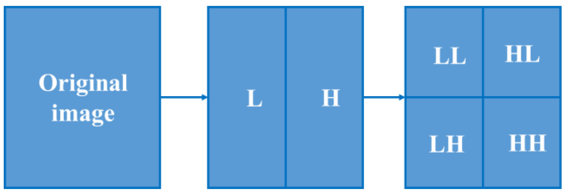
2. Structured Light Measurement System and QWT Denoising Algorithm

A 3D structured light measurement system is shown in Figure 2. Oc is the center point of the image sensor, Or is the center of the projector, and $P(x,y)$ is any point of the measured object. Suppose that a beam of light QrB from the projector is projected on point B on the reference plane, and the light beam is projected on point P of the object because of the existence of the object under testing. From the point of view of the sensor, when there is no object to be measured, point A on the reference plane images a point $(m,n)$ on the sensor array, and point A carries the information of the QrA light from the projector. Due to the existence of the measured object, point P on the object is imaged to the $(m,n)$ of the sensor array, and P carries the information of the light OrB. Therefore, the distance from A to B, expressed as s, carries the information of the height $h(x,y)$ of the object at $P(x,y)$. $h(x,y)$ can be calculated by

$$h(x,y)=\frac{ls(x,y)}{d+s(x,y)}.$$

(1)

where d is the distance between the image sensor and projector, and l is the vertical distance from the projector to the reference plane. The spatial period of sinusoidal fringes on the xoy plane is ${\lambda }_0$. The light intensity of points A and B on the xoy plane can be expressed as

$$I_0=a(x,y)+b(x,y)cos[2\pi {\lambda }_{0}x+{\varphi }_A(x,y)],$$

(2)

$$I=a(x,y)+b(x,y)cos[2\pi {\lambda }_{0}x+{\varphi }_B(x,y)].$$

(3)

s can be obtained by

$$s(x,y)=\frac{({\varphi }_A-{\varphi }_B){\lambda }_0}{2\pi }=\frac{\mathsf{\Delta }\varphi {\lambda }_0}{2\pi }.$$

(4)

Thus, $h(x,y)$ can be calculated by

$$h(x,y)=\frac{l({\varphi }_A-{\varphi }_B)}{({\varphi }_A-{\varphi }_B)+2\pi d/{\lambda }_0}.$$

(5)

Figure 2. Structured light 3D profile measurement system.

Figure 2. Structured light 3D profile measurement system.

The phases ${\varphi }_A(x,y)$ and ${\varphi }_B(x,y)$ need to be extracted from the sinusoidal fringe image captured by the image sensor by the multistep phase-shifting method. N sinusoidal fringe images from the projector by phase-shifting can be described by

$$I_i(m,n)=I_0(m,n)+\gamma (m,n)cos[\varphi (m,n)+{\alpha }_i],i=1,2,\dots ,N$$

(6)

where i is the number of phase shifts, $I_0(m,n)$ is the background gray level, $\gamma (m,n)$ is the modulation depth, ${\alpha }_i$ is the phase of the i-th shift, and $\varphi (m,n)$ is the phase obtained and can be obtained by

$$tan\varphi (m,n)=\frac{{\displaystyle \sum _{n=1}^N}{I}_n(m,n)(sin[2\pi (n-1)/N])}{{\displaystyle \sum _{n=1}^N}{I}_n(m,n)(cos[2\pi (n-1)/N])}.$$

(7)

By using the four-step phase-shifting method, ${\alpha }_1=0$, ${\alpha }_2=\pi /2$, ${\alpha }_3=\pi$, and ${\alpha }_4=3\pi /2$, Equation (7) becomes

$$tan\varphi (m,n)=\frac{I_4(m,n)-I_2(m,n)}{I_1(m,n)-I_3(m,n)}.$$

(8)

According to Equations (1)–(8), $h(x,y)$ is determined by $\varphi (x,y)$, which can be achieved by phase unwrapping. Sinusoidal modulated fringe images contain various types of noise, which affect the accuracy of phase unwrapping. Therefore, before phase unwrapping, it is necessary to denoise the images. The principle of image denoising is to remove all kinds of noise in the image as much as possible, such as Gaussian white noise and salt and pepper noise, while keeping the original image information from loss to the greatest extent possible.

The 2D-DWT decomposition schematic diagram is shown in Figure 3. For every fringe image, one-dimensional (1D) discrete WT (DWT) according to the row of fringe images is carried out, and the L subband or H subband is achieved. Then, one low-frequency subband (LL) and three horizontal (LH), vertical (HL), and diagonal (HH) subbands are obtained by 1D DWT according to the column of L and H subbands. The coefficient for the four subbands is expressed by the real function $f(x,y)$.

As shown in Figure 4, this quaternion wavelet analysis comes from four real-coefficient DWTs. The first DWT corresponds to the real part of the quaternion wavelet analytical signal, $f^q(x,y)$, and the second and third correspond to the first wavelet processed with a partial Hilbert transformation along the horizontal and vertical directions, which are expressed as $H_{Hx}\left[f\left(x,y\right)\right]$ and $H_{Hy}\left[f\left(x,y\right)\right]$, respectively. The last wavelet is obtained from the first wavelet processed with the whole Hilbert transform, and it is expressed as $H_{Hxy}\left[f\left(x,y\right)\right]$. $H_{Hx}\left[f\left(x,y\right)\right]$, $H_{Hy}\left[f\left(x,y\right)\right]$, and $H_{Hxy}\left[f\left(x,y\right)\right]$ correspond to the three imaginary parts, $i,j,k$, of the quaternion wavelet, respectively. Each discrete wavelet analysis can be divided into two parts: decomposition and reconstruction. Each decomposition part can be regarded as a two-dimensional dual-tree complex wavelet transformation. A one-dimensional dual-tree complex wavelet transformation was performed on the rows, and another one-dimensional dual-tree complex wavelet transformation was performed on the columns. In the decomposition operation, the dual-tree filter is adopted with downsampling, including filters $h_0$, $h_1$, $g_0$, and $g_1$, respectively. After decomposition, we can obtain sixteen subsections: $LL$, $LH$, $HL$, $HH$, $L{L}_i$, $L{H}_i$, $H{L}_i$, $H{H}_i$, $L{L}_j$, $L{H}_j$, $H{L}_j$, $H{H}_j$, $L{L}_k$, $L{H}_k$, $H{L}_k$, and $H{H}_k$. After the above wavelet decomposition, a quaternion wavelet can be obtained, and it is expressed as follows:

$$f^q(x,y)=f(x,y)+i{H}_{H\mathrm{x}}\left[f(x,y)\right]+j{H}_{H\mathrm{y}}\left[f(x,y)\right]+k{H}_{Hxy}\left[f(x,y)\right].$$

(9)

Wavelet decomposition can be continued according to the route described above. To select the level of the multilevel quaternion wavelet, the denoising effect, computational complexity, and time consumption should be taken into account. When the number of decomposition layers increases, the complexity increases exponentially. Moreover, if the number of decomposition layers is too large, the image will be too smooth and lose the texture details. Thus, we use a three-level quaternion decomposition.

Then, quaternion $f^q(x,y)$ can also be written in another form:

$$f^q(x,y)=\left|f^q(x,y)\right|e^{j\phi }{e}^{j\theta }{e}^{j\psi }.$$

(10)

where $|f^q(x,y)|$ is the modulus of $f^q(x,y)$, and $\phi ,\theta ,\psi$ are three phase angles that are uniquely defined within the range $(\phi ,\theta ,\psi )\in [\pi ,\pi ]\times [-\pi /2,\pi /2]\times [-\pi /4,\pi /4]$. The quaternion wavelet corresponds to one magnitude and three phases, which can be depicted in the four images shown in Figure 5. The QWT results indicate that three phase images mainly reflect the edge and texture information of the image, which are randomly and disorderly distributed to the noise, while the amplitude image is greatly affected by the noise. Therefore, the principle of denoising is that the amplitude coefficients are processed according to a certain criterion, and the phase coefficients remain. For amplitude images, most of the energy is concentrated on a small number of coefficients with large amplitudes, which represent the edge and other details. The noise mainly corresponds to coefficients with smaller amplitudes. It is reasonable to set a certain threshold to reduce the noise in the amplitude image. The following steps are performed to remove amplitude noise. First, the variance of noise according to the robust estimation method is calculated by [19]

$${\sigma }_{n^{{}^{\prime }}}=\frac{Median\left(\right|{\omega }_{i,j}\left|\right)}{0.6745}.$$

(11)

where ${\omega }_{i,j}$ is the finest subband coefficient, and $|{\omega }_{i,j}|$ denotes its magnitude. Then, the amplitude variance ${\sigma }_w^2$ is estimated by

$${\sigma }_w^2=\frac{1}{N^2}\sum _{|{\omega }_j|\in W\left(k\right)}{\left(\right|{\omega }_j\left|\right)}^2.$$

(12)

where $W\left(k\right)$ is the square-shaped neighborhood window of $|{\omega }_j|$, and $N^2$ is the size of the window. Therefore, QWT coefficients can be obtained by

$$\omega =m^{{}^{\prime }}+n^{{}^{\prime }}.$$

(13)

where $\omega$, $m^{{}^{\prime }}$, and $n^{{}^{\prime }}$ are matrices of the observed QWT coefficients, ideal QWT coefficients, and noise QWT coefficients, respectively. Variance ${\sigma }_{m^{{}^{\prime }}}$ can be estimated by

$${\sigma }_{m^{{}^{\prime }}}=\sqrt{max({{\sigma }_w}^2-{{\sigma }_{n^{{}^{\prime }}}}^2,0)}.$$

(14)

Third, a shrink threshold needs to be determined. For each subband in the QWT domain, if the threshold is too low, then the denoising effect is not obvious. If the threshold is too high, then more details will be “killed’’. Therefore, a reasonable noise-free coefficient’s magnitude m is required by using the Bayes shrink threshold T [20]

$$T=\frac{{\sigma }_{n^{{}^{\prime }}}^2}{{\sigma }_{m^{{}^{\prime }}}}.$$

(15)

Fourth, the element of coefficients matrix m can be determined by the soft thresholding function

$$m_{k,j}^i=\left\{\begin{array}{c}sign\left(w_{k,j}^i\right)\times \left(\right|w_{k,j}^i|-T_{k,j}^i),if|w_{k,j}^i|>T_{k,j}^i\hfill \\ 0,else\hfill \end{array}\right.$$

(16)

where ${\omega }_{k,j}^i$ is the ith coefficient in the j direction of the k layer, $T_{k,j}^i$ is the corresponding threshold, and $m_{k,j}^i$ is the coefficient after denoising.

Finally, by performing an inverse QWT on the estimated magnitude and the original phase to obtain QWT coefficients, four denoised sinusoidal modulated fringe images can be reconstructed. After QWT denoising, the phase unwrapping algorithm can be applied to the denoised sinusoidal modulation fringe images.

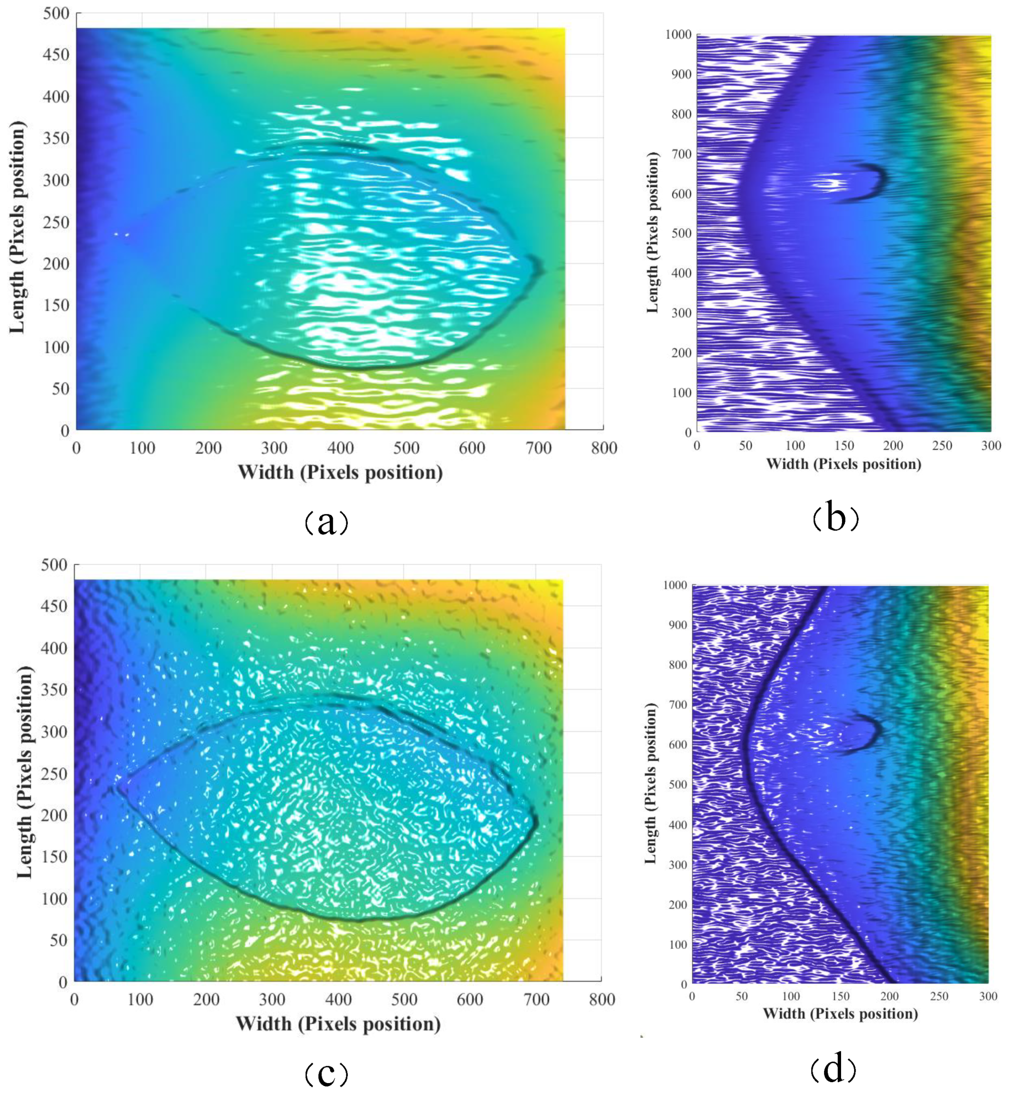
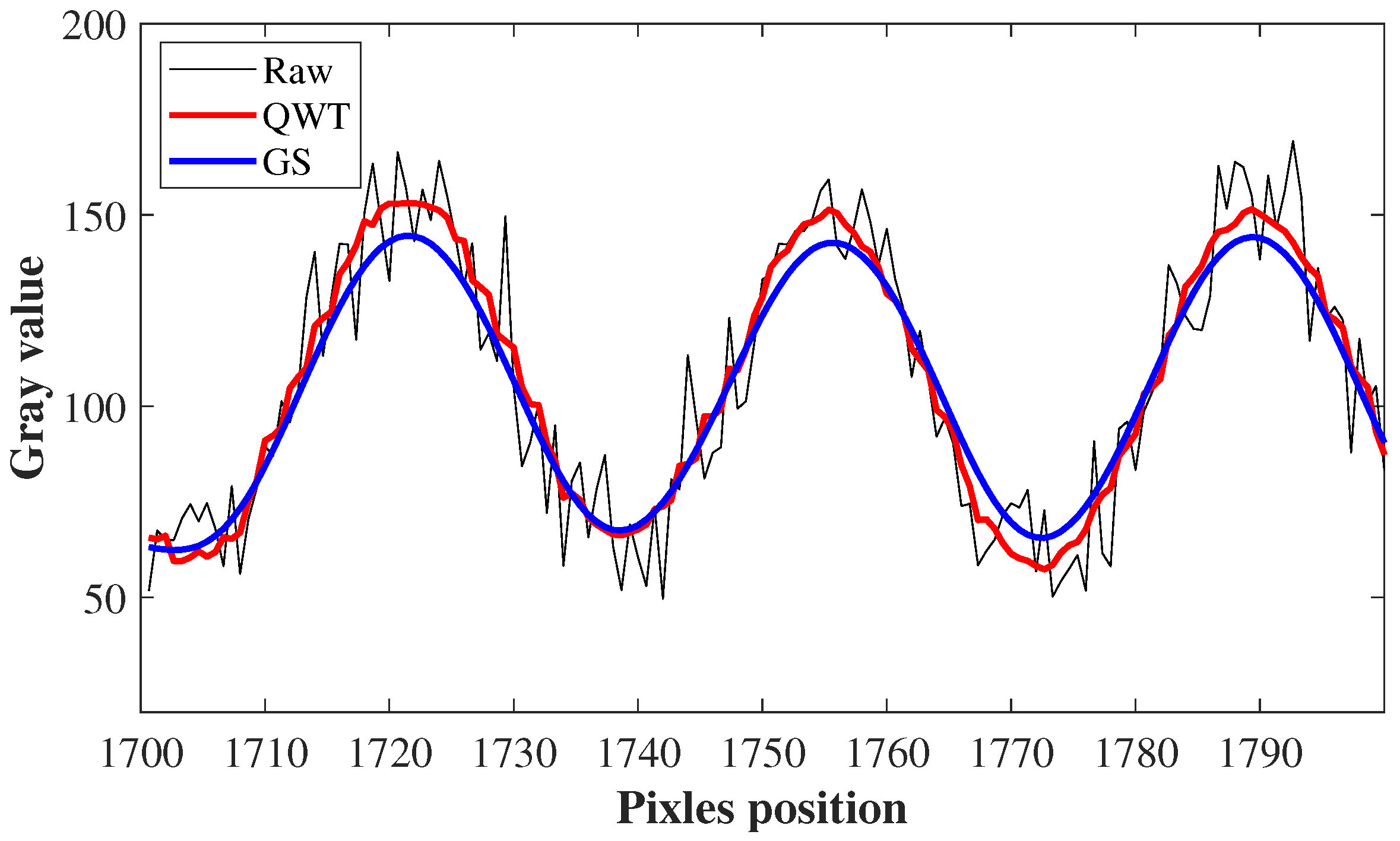
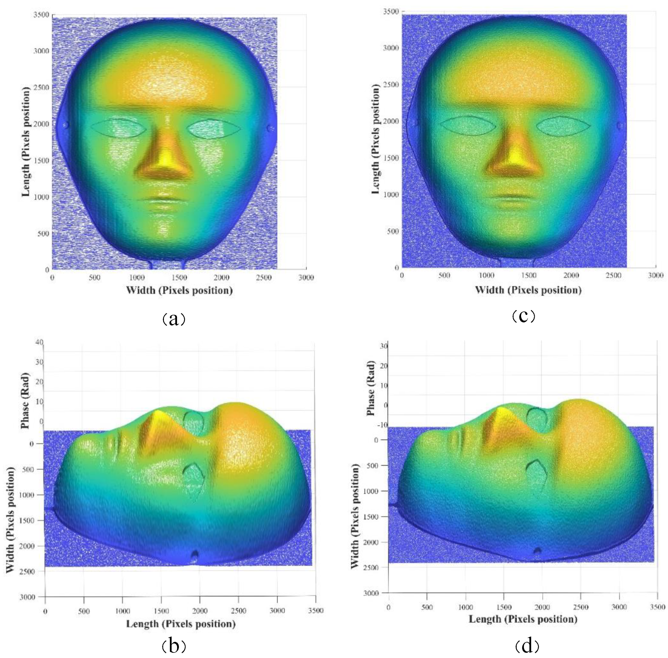
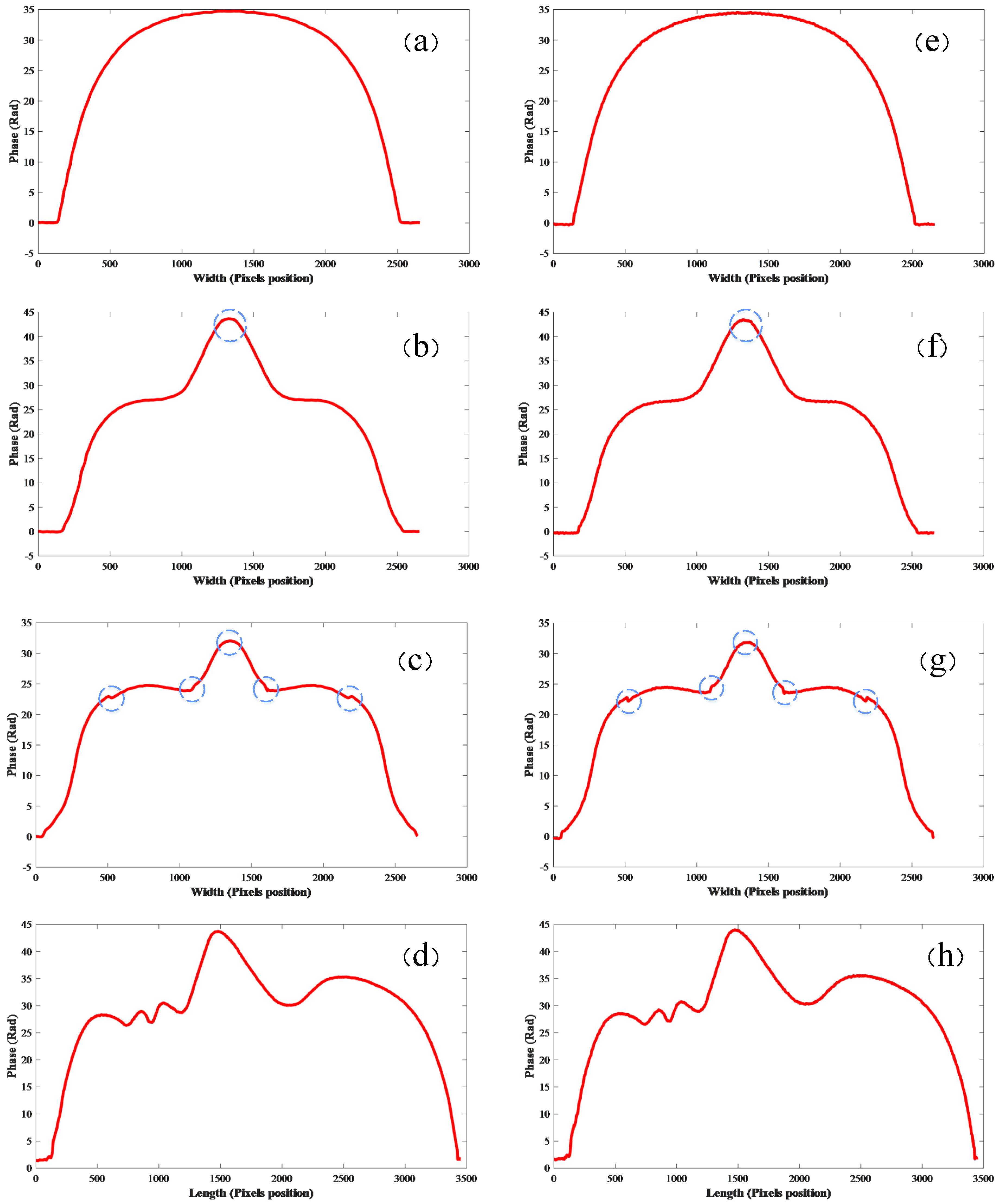
3. Results and Discussion

In the measurement system shown in Figure 2, the distance between the projector and the reference white screen is 80 cm, the image sensor contains 2592 × 3872 pixels, and an Acer D606D projector is selected. By using the dual-frequency heterodyne method, the sinusoidal fringes with 128 and 127 periods are generated by the computer and then projected to the reference white screen and the measured objects by four-step phase-shifting. The quantization bit of the image sensor is 8 bits. Parameters such as the brightness and contrast of the projector are properly adjusted to keep the quantization interval between 20 and 240. Due to the large amount of white Gaussian noise in the images, to highlight the performance advantages of QWT denoising, we choose the GS denoising algorithm for comparison. To balance the denoising and measurement accuracy, a smoothing window of 50 × 50 is selected for the GS denoising algorithm. To evaluate the denoising effect of the QWT algorithm, we first select an image on the reference screen for analysis. Parts of the raw sinusoidal fringe image and its corresponding result processed by the GS and QWT denoising algorithms are shown in Figure 6. After a simple visual inspection of the three images, it is found that the original sinusoidal fringe image is almost covered by white or black noise points, while the noise points are almost completely removed in the denoised images. The fringes after denoising by GS have some clear vertical “scratches”, while those processed by QWT denoising are very smooth and natural. The denoising effect of the algorithm can also be evaluated quantitatively by the standard deviation (SD) and SNR. The calculated results show that the SD is 0.1448 for the raw image and 0.0282 and 0.0192 for the denoised images of the GS and QWT algorithms, respectively. The SNR of 4.6213 dB obtained from the raw image can be substantially boosted to 11.6759 dB and 13.3463 dB by applying the GS and QWT denoising algorithms, respectively. Therefore, intuitively, the denoising effect of QWT is better than that of the GS denoising algorithm.

The performance of denoising algorithms can also be evaluated by the shape of the extracted curves. Figure 7 shows the curves extracted from the raw sinusoidal fringe image on the reference white plane and the corresponding denoised results by the GS and QWT algorithms. The smoothing window for the GS denoising algorithm is 50 × 50. The gray distribution curves processed by the two methods maintain a good sinusoidal in shape, and gray distribution curves for GS are relatively smooth, while that for QWT has little “spurs”. However, this will cause more feature information denoised by GS, such as edge and texture, to be potentially lost.

Because the reference white screen contains less image information, we also choose the results of phase unwrapping of the reference plane to investigate the denoising effect of the two algorithms on the image with less information. Figure 8 shows the principal phase distributions of unwrapping obtained by GS and QWT denoising. The phase distributions of the principal value obtained by the two algorithms are almost identical; this shows that the QWT algorithm can achieve the same denoising effect as the GS algorithm with a 50 × 50 smoothing window for the smooth region without edge, texture, and other feature information.

To further compare the differences of various denoising algorithms, a group of face mask images being projected with different phase sinusoidal fringes are unwrapped. The raw image and results of phase unwrapping with raw data are shown in Figure 9. Two-dimensional Fourier analysis for the original image must be carried out first; then, the frequency domain of the image is determined according to the analysis results, and frequency domain filtering is performed for the interval beyond the frequency domain range of the image. The same frequency domain range is adopted after the images are denoised by the GS or QWT algorithms. Due to the serious noise in raw images, although all sinusoidal fringe images are filtered in the frequency domain, the phase unwrapping accuracy is relatively low, there are many phase error areas at the mask edge, and it is difficult to recover by the phase error correction algorithm. Therefore, it can be concluded that image denoising must be carried out first for a 3D measurement in a high noise environment.

The different angle 3D contours of phase unwrapping obtained from the images by using the GS and QWT denoising algorithms are shown in Figure 10. Almost no phase unwrapping errors were found in the 3D contours from GS, while the phase of all the points on the face mask is correct except for some sporadic phase errors at the edge. These incorrect phase points can be easily detected and corrected. Intuitively, the result of GS is relatively stiff and lacks texture. In contrast, that from the QWT looks natural and closer to the real face mask. The SDs for the 3D mask are 0.0239 and 0.0502 from the GS algorithm and the QWT algorithm, respectively. Quantitatively, the overall denoising effect of the two algorithms is almost the same.

Although GS has achieved a good denoising effect in areas with less information, such as the forehead, it is not satisfactory in areas with rich information, such as eyes and edges. The details of the eyes and edge of the face mask from GS and QWT are shown in Figure 11. The eyelids and edge become blurred because of the weighted mean processing in the Gaussian smoothing algorithm with a 50 × 50 window. Because of the effective separation of noise and information in the QWT denoising algorithm, the useful information can be retained as much as possible while removing the noise, and the details of the eyelids and edge of the mask from the QWT are very clear.

To further investigate the influence of the denoising algorithm on the measurement accuracy, we extract the cross-sectional curves of different parts of the face mask, which come from the results of phase unwrapping by using the GS and QWT denoising algorithms, and the results are shown in Figure 12. For the regions with less information, such as the forehead and nose, the cross-sectional curves obtained by the two methods are almost the same. For the parts with a large amount of information, such as the eyes, the changes in eyelids obtained by the GS algorithm are relatively gentle, while those obtained by the QWT algorithm are relatively steep. Quantitatively, the thickness of the eyelid from the GS algorithm is 0.681 mm, and the width of coverage between the lowest point and the highest point is 1.59 mm, but for the QWT algorithm, the thickness of the eyelid is 1.99 mm, and the width of coverage is 0.47 mm. The result by QWT is consistent with the actual 2 mm mask thickness. At the widest part of the mask, the width value from the results of the QWT algorithm is 160.01 mm, while it is 160.53 mm for the GS algorithm. For the curves of the vertical section, the maximum distance from the results of the GS algorithm is 220.02 mm, and that for the QWT algorithm is 220.27 mm. All values obtained by using the QWT are consistent with the actual size of the mask: 220 × 160 × 60 mm. The results obtained by the GS algorithm have obvious deviations. Therefore, for 3D measurements of complex structure surfaces, when the required measurement accuracy is very high, the QWT algorithm is suitable for denoising sinusoidal fringe images full of noise.

The efficiency of the algorithm can be evaluated by the running time of the algorithm on the computer. It takes approximately 16 s to run the GS algorithm to process eight pairs of sinusoidal fringe images with 2592 × 3872 pixels, while it takes less than 20 s for the QWT algorithm, which can meet the requirements of most high-precision measurements. Finally, we have summarized the whole numerical results as shown in

Table 1. Comparison between Gauss algorithm and QWT algorithm.

Algorithm	SD for Images	SNR	SD for Mask	Thickness	Coverage	Width	Running Time
GS	0.0282	11.6759 dB	0.0239	0.681 mm	1.59 mm	160.53 mm	16 s
QWT	0.0192	13.3463 dB	0.0502	1.99 mm	0.47 mm	160.01 mm	20 s

. The QWT is more efficient.

4. Conclusions

A QWT denoising algorithm is proposed to process the sinusoidal fringe images collected by array image sensors in a structured light 3D profile measurement system. Theoretical analysis shows that noise and useful information can be effectively separated after the image is decomposed by the quaternion wavelet. Then, a soft threshold function is introduced to remove the noise in the amplitude image of the quaternion wavelet, and the phase image with useful information remains. According to the theoretical results, the QWT denoising algorithm is suitable for image denoising during precise measurements of 3D contours for complex structures. A structured light 3D profile measurement system is set up to demonstrate the proposed denoising algorithm, and the classical GS denoising algorithm is used for comparison. For a sinusoidal fringe image with substantial noise, the processing results of the two algorithms indicate that the SD is reduced from 0.1448 for the raw image to 0.0282 and 0.0192, and the SNR is boosted from 4.6213 dB for the raw image to 11.6759 dB and 13.3463 dB by applying the GS and QWT denoising algorithms, respectively. The extracted curve from the image denoised by GS has some small “burrs”, while the curve from the image denoised by GS is very smooth and is similar to a sine wave in shape. The results of phase unwrapping indicate that the results obtained by the two denoising methods are almost the same for the surface with less information. For a surface with rich information, the image blur introduced by GS will cause a loss of surface details, especially at the edge of the structure. However, using the sinusoidal fringe image denoised by the QWT algorithm, the details of the 3D contour of a complex structure can be recovered completely, and for the measured face mask, the error is less than ±0.02 mm. In the application of real 3D imaging, CCD will inevitably show jitter and error when the object is in dynamic motion. The result of our work provides the possibility of a theoretical scheme for noise reduction in 3D imaging, but we believe that the QWT denoising algorithm will play a role in 3D precision measurements of complex structures.

References

1. Stickland, M.; McKay, S.; Scanlon, T. The development of a three dimensional imaging system and its application in computer aided design workstations. Mechatronics 2003, 13, 521–532. [Google Scholar] [CrossRef]
2. Xinmin, L.; Zhongqin, L.; Tian, H.; Ziping, Z. A study of a reverse engineering system based on vision sensor for free-form surfaces. Comput. Ind. Eng. 2001, 40, 215–227. [Google Scholar] [CrossRef]
3. Spagnoloa, G.S.; Ambrosinib, D.; Paolettib, D.; Accardoc, G. Fibre optic projected fringes for monitoring marble surface status. J. Cult. Herit. 2000, 1, S337–S343. [Google Scholar] [CrossRef]
4. Tepper, O.M.; Small, K.; Rudolph, L.; Choi, M.; Karp, N. Virtual 3-dimensional modeling as a valuable adjunct to aesthetic and reconstructive breast surgery. Am. J. Surg. 2006, 192, 548–551. [Google Scholar] [CrossRef] [PubMed]
5. Jarvis, R.A. A Laser Time-of-Flight Range Scanner for Robotic Vision. IEEE Trans. Pattern Anal. Mach. Intell. 1983, 5, 505–512. [Google Scholar] [CrossRef] [PubMed]
6. Li, C.; Wang, Y.; Wang, J.; Yao, H.; Liu, X.; Gao, R.; Yang, L.; Xu, H.; Zhang, Q.; Ma, P.; et al. Convolutional Neural Network-Aided DP-64 QAM Coherent Optical Communication Systems. J. Light. Technol. 2022, 40, 2880–2889. [Google Scholar] [CrossRef]
7. Jalkio, J.A.; Kim, R.C.; Case, S.K. Three Dimensional Inspection Using Multistripe Structured Light. Opt. Eng. 1985, 24, 966–974. [Google Scholar] [CrossRef]
8. Qian, J.; Feng, S.; Tao, T.; Hu, Y.; Liu, K.; Wu, S.; Chen, Q.; Zuo, C. High-resolution real-time 360 3D model reconstruction of a handheld object with fringe projection profilometry. Opt. Lett. 2019, 44, 5751–5754. [Google Scholar] [CrossRef] [PubMed]
9. Wu, G.; Wu, Y.; Li, L.; Liu, F. High-resolution few-pattern method for 3D optical measurement. Opt. Lett. 2019, 44, 3602–3605. [Google Scholar] [CrossRef] [PubMed]
10. Wu, Z.; Guo, W.; Zhang, Q. High-speed three-dimensional shape measurement based on shifting Gray-code light. Opt. Express 2019, 27, 22631–22644. [Google Scholar] [CrossRef] [PubMed]
11. Yin, W.; Feng, S.; Tao, T.; Huang, L.; Trusiak, M.; Chen, Q.; Zuo, C. High-speed 3D shape measurement using the optimized composite fringe patterns and stereo-assisted structured light system. Opt. Express 2019, 27, 2411–2431. [Google Scholar] [CrossRef] [PubMed]
12. Zhang, C.; Duan, F.J. Phase stepping methods based on PTDC for Fiber-Optic Projected-Fringe Digital Interferometry. Opt. Laser Technol. 2012, 44, 1089–1094. [Google Scholar]
13. Wang, Y.; Yao, H.; Wang, J.; Xin, X. Distributed Optical Fiber Sensing System for Large Infrastructure Temperature Monitoring. IEEE Internet Things J. 2022, 9, 3333–3345. [Google Scholar] [CrossRef]
14. Gai, S.; Yang, G.; Zhang, S. Multiscale texture classification using reduced quaternion wavelet transform. AEU—Int. J. Electron. Commun. 2013, 67, 233–241. [Google Scholar] [CrossRef]
15. Liu, Y.; Jin, J.; Wang, Q.; Shen, Y. Phase-preserving speckle reduction based on soft thresholding in quaternion wavelet domain. J. Electron. Imaging 2012, 21, 043009. [Google Scholar] [CrossRef]
16. Chai, P.; Luo, X.; Zhang, Z. Image Fusion Using Quaternion Wavelet Transform and Multiple Features. IEEE Access 2017, 5, 6724–6734. [Google Scholar] [CrossRef]
17. Yin, Y.; Wu, K.; Lu, L.; Song, L.; Zhong, Z.; Xi, J.; Yang, Z. High dynamic range 3D laser scanning with the single-shot raw image of a color camera. Opt. Express 2021, 29, 43626–43641. [Google Scholar] [CrossRef]
18. Zhou, P.; Zhu, J.; Xiong, W.; Zhang, J. 3D face imaging with the spatial-temporalcorrelation method using a rotary speckle projector. Appl. Opt. 2021, 60, 5925–5935. [Google Scholar] [CrossRef] [PubMed]
19. Donoho, D.; Johnstone, I. Ideal Spatial Adaptation by Wavelet Shrinkage. Biometrika 1998, 81, 425–455. [Google Scholar] [CrossRef]
20. Chang, S.; Yu, B.; Vetterli, M. Adaptive Wavelet Thresholding for Image Denoising and Compression. IEEE Trans. Image Process. 2000, 9, 1532–1546. [Google Scholar] [CrossRef] [Green Version]
Figure 1. Algorithmic Operation Flowchart.
Electronics 11 01807 g001
Figure 3. Image wavelet decomposition schematic diagram.
Electronics 11 01807 g003
Figure 4. Quaternion wavelet principle.
Electronics 11 01807 g004
Figure 5. Results of decomposition by QWT: (a) magnitude and (bd) the 3 terms of phase ( φ , θ , ψ ).
Electronics 11 01807 g005
Figure 6. Raw sinusoidal fringe image (a) and the processing of corresponding results by using GS (b) and QWT (c).
Electronics 11 01807 g006
Figure 7. Curves extracted from different images.
Electronics 11 01807 g007
Figure 8. Principal phase distributions of phase unwrapping by using GS (a) and QWT (b).
Electronics 11 01807 g008
Figure 9. Face mask (a) and its 3D contour of phase unwrapping from raw images (b).
Electronics 11 01807 g009
Figure 10. Results of mask phase unwrapping via the GS denoising algorithm: frontal face (a,b) side face; results of mask phase unwrapping via the QWT denoising algorithm: frontal face (c,d) side face.
Electronics 11 01807 g010
Figure 11. Details of eyelids (a) and edges (b) by using using the GS algorithm; details of eyelids (c) and edges (d) by the QWT algorithm.
Electronics 11 01807 g011
Figure 12. Cross-sectional curves of the forehead (a), nose (b), eye (c), and vertical section curve (d) by using GS algorithm. Cross-sectional curves of the forehead (e), nose (f), eye (g), and vertical section curve (h) by using QWT algorithm.
Electronics 11 01807 g012