Force Tracking Control of Functional Electrical Stimulation via Hybrid Active Disturbance Rejection Control

Abstract

Stroke is a worldwide disease with a high incidence rate. After surviving a stroke, most patients are left with impaired upper or lower limb. Muscle force training is vital for stroke patients to recover limb function and improve their quality of life. This paper proposes a force tracking control method for upper limb based on functional electrical stimulation (FES), which is a promising rehabilitation approach. A modified Hammerstein model is proposed to describe the nonlinear dynamics of biceps brachii, which consists of a nonlinear mapping function, linear dynamics and time delay component to represent the biochemical process of muscle contraction. A quick model identification method is presented based on the least square algorithm. To deal with the variation of muscle dynamics, a hybrid active disturbance rejection control (ADRC) is proposed to estimate and compensate for the model uncertainty and unmeasured disturbances. The parameter tuning process is given. In the end, the performance of the proposed methods is verified via simulations and experiments. Compared with the Proportional integral derivative controller (PID) method, the proposed methods could suppress the model uncertainty and improve the tracking precision.

1. Introduction

Stroke is a disease with a high incidence rate and high disability rate considered at a global level. Almost fifteen million people suffer a stroke worldwide, and only 5% of survivors with severe disability regain upper–limb function [1], and 50% to 80% of survivors have varying degrees of disabling sequelae in China [2]. Most stroke patients without rehabilitation are at risk of muscular dystrophy [3]. Functional electrical stimulation (FES) is a promising approach for motor rehabilitation, and is carried out by applying artificial stimulation to muscles and nervous system to enable functional training. FES has been applied to hand rehabilitation [4], upper limb rehabilitation [5,6,7,8], treadmill walking [9], FES–cycling [10] and so on. Those applications focus on motor rehabilitation, though muscle force training could improve motor function significantly [11]. Furthermore, muscle force control could be regarded as an inner–loop in the closed–loop motion control of motor rehabilitation [12], and a precise force tracking control benefits the performance of motor rehabilitation. For those reasons, we develop a muscle force tracking control system in this article.

The target of the proposed system is to impel the output force of selected muscle to track a given reference. The output force is derived from the contraction of muscle fibers which are activated by the artificial stimulation applied by FES and involve complex electrophysiological process [12]. It is almost impossible to build a precise mechanism model of a musculoskeletal system, and models widely used in this art are empirical models, such as Hill–Type models [13] and their modifications [14], the neural network model [15] and the Hammerstein model [16]. Consisting of piecewise nonlinear functions, Hill–Type models could fit the experimental data precisely [17], but it is not easy to be identified and applied to the control system design. The neural network model only needs input and output data. However, enormous data is required for the fitting of neural network [18]. Different from the Hill–Type model, the Hammerstein model comprises a static nonlinear function followed by a dynamic linear block, and could be identified efficiently [19,20]. There is a time–varying input delay between the application of electrical stimulation and the corresponding muscle contraction, which is caused by the electrochemical process and named as electromechanical delay (EMD) [21]. EMD is critical to the closed–loop control performance, and can even destabilize the control system. Although EMD has been explored and modeled [21,22], it has not been fully used to improve closed–loop control performance. In this paper, a musculoskeletal model combining the Hammerstein model and EMD is proposed. Based on the proposed model, a closed–loop control method is proposed to achieve a precise force tracking control.

Different control methods have been applied to the control of FES system, such as PID and their modifications [23], adaptive fuzzy terminal sliding mode control method [24], reinforcement learning method [7], neural network based modeling and control method [25], iterative learning control method [26], multiple–model adaptive control method [16], etc. However, none of those methods took EMD into account. PID with delay compensation method [27] and a closed–loop method robust to unknown time–varying EMD [28] were proposed to deal with EMD, although in those research the dynamics of muscle contraction was omitted, and the modeling precision and the control performance were deteriorated inevitably. Affected by characteristics and status of a musculoskeletal system, the musculoskeletal model varies from person to person, even from time to time. To deal with the variation, adaptive control [16,29] and robust control methods [30,31] are applied, in which the structure or boundary uncertainties are assumed to be known. In this work, active disturbance rejection control (ADRC) is employed and improved to estimate and compensate for the model error, and then a precise force tracking control is realized.

ADRC is proposed in [32] and improved in [33,34], which consists of tracking differentiators (TD), non–linear state error feedback (NLSEF) and extended state observe (ESO). The external disturbance and unmodeled system dynamics are regarded as an extended state and estimated by ESO, then compensated to the control loop. With this mechanism, a vast range of uncertainties could be dealt with, releasing the requirement of a precise mathematical model [35]. ADRC has drawn considerable attention and has been applied to many applications, such as superheated steam temperature control [36,37], flight control [38], etc. For the time delay systems, several methods based on ADRC have been proposed, such as increasing order method [39], predictive input/output method [40], and delayed input method [41]. The first method increases the order of the plant model to approximate the time delay, while the second method designs a predictor to eliminate the effect of time delay, the two methods will increase the controller’s complexity. Compared with the first two methods, only a time delay module is added to ESO in the last one. In this article, the last method is employed to reduce the effect of EMD.

The objective of this article is to propose a modeling method and a precise force tracking control on healthy participants. These proposed methods have the potential to be applied to unhealthy participants and improve the performance of FES–induced rehabilitation. For this purpose, three contributions are made as follows:

• A modified Hammerstein model, including nonlinear mapping function, linear dynamics and EMD, is proposed and used to model the nonlinear dynamics of biceps. The three parts of the proposed model are identified respectively. To speed up the identification process, a fast identification method is presented, in which the linear dynamics and EMD are identified only one time for a participant. In contrast, the nonlinear mapping function will be identified before each experiment.
• A hybrid ADRC method is presented, in which the inverse of the static nonlinear function is cascaded into the control loop to attenuate the nonlinearity of the musculoskeletal system, and a delayed input module is added to reduce the effect of EMD. The controller parameters will be constant once tuned according to the identified model.
• The performance of the proposed methods is verified by experiments and comparisons with the traditional PID method. These results indicate that the proposed methods could be used to improve the FES–induced motion rehabilitation performance of closed–loop controllers that are insensitive to time–varying musculoskeletal characteristics.

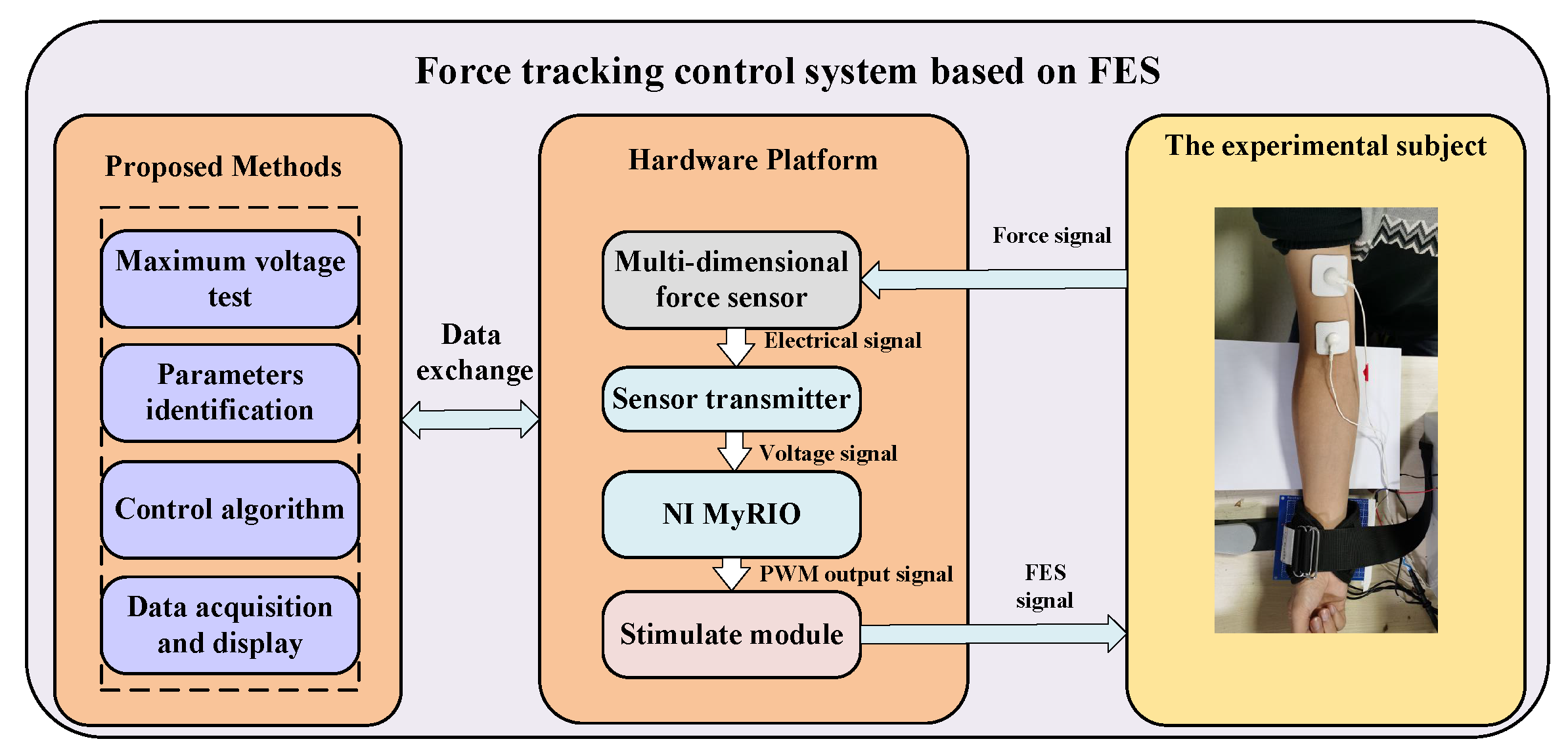
The rest of the paper is arranged as follows: Section 2 establishes a parameterized nonlinear biceps brachii musculoskeletal model with Hammerstein structure, and a hybrid ADRC consisting of feedforward control and time delay synchronization is put forward. Simulation and experiments are executed in Section 3 to verify the performance of proposed methods. Finally, Section 4 summarizes the paper and draws conclusions.

2. System Overview

2.1. Experimental Setup

To realize precise muscle force control, an experimental platform is set up as shown in Figure 1, which consists of the hardware system and software system. All methods proposed in this paper are verified on this platform. To make this paper more readable, a brief introduction of the hardware system and software system are first given.

In the hardware system, there are mainly four parts, i.e., multi–dimensional force sensor, sensor transmitter, controller (NI MyRIO 1900) and multi–channel electrical stimulator module. Three component forces are measured by the multi–dimensional force sensor, and then enlarged and filtered by the sensor transmitter. The analog signals of the three component forces are converted to digital signals via an analog–digital converter in NI MyRIO. Then, the output force of the muscle, the resultant force of the three component forces, is calculated. The control signal generated by a controller running on NI MyRIO is transmitted to the multi–channel electrical stimulator and applied to the biceps brachii muscle of experimental subjects via electrode pads.

The software system is implemented in LabVIEW and running on the NI MyRIO. The software system consists of four parts, which are maximum stimulus voltage test module, parameters identification module, ADRC controller, and data acquisition and display module. The voltage threshold of FES varies from person to person due to interpersonal differences in skin features and pain tolerance. Thus, it is necessary to determine the maximum stimulus voltage before carrying out any experiment. The second module is used to identify the parameters of nonlinear mapping function, which is the most critical composition of the proposed modified Hammerstein model based on which the ADRC controller is designed. The ADRC controller generates the control signal according to the error between the reference force and the output of biceps brachii muscle. The last module acquires data of the platform i.e., reference signal, the output force of biceps, the control signal, and displays these information to the user. The above modules constitute the closed–loop control system shown in Figure 2.

2.2. Modified Hammerstein Model and Parameter Identification

A precise model could improve the control accuracy dramatically. However, due to the unknown electrophysiological process and lack of a sensing approach for muscle fiber states in vivo, it is almost impossible to model the dynamics of biceps brachii muscle precisely. To obtain a more precise biceps model and to balance the model parameter identified complexity and ease–of–use, a modified Hammerstein model is proposed, which takes the time delay characteristic of biceps into consideration. The model parameters identification method is given and verified via experiments.

2.2.1. Modified Hammerstein Model

The proposed model consists of a nonlinear mapping function, linear dynamics and time delay as shown in Figure 3.

The nonlinear mapping function, which is also named as isometric recruitment curve (IRC), represents the nonlinear response of biceps brachii muscle to FES. To analyze and describe the nonlinear response, four participants’ biceps are stimulated by a sinusoidal signal of which the period is much larger than the rise time of the linear dynamics, and the amplitudes are participants’ maximum stimulus voltage and varies from person to person, then the output signal is recorded. The results are shown in Figure 4a, whose horizontal axis represents the duration of a pulse–width modulation (PWM) voltage generator, of which the PWM period is constant at 40 ms. The vertical axis represents the force generated by participants’ biceps muscle. There are four curves representing the response of four participants. Though the curves are different from each other significantly, they are in the same shape, that is, the S–curve. A polynomial function is used to fit the S–curve, that is,

$$f\left(u\right)=c_0+c_{1}u+c_2{u}^2+c_3{u}^3+\dots +c_q{u}^q,$$

(1)

where u is the control input of FES, $c_0$, $c_1$, $c_2$, …, $c_q$ represent the coefficients of the IRC.

The linear dynamics, i.e., linear activation dynamics (LAD), models the dynamical characteristics of biceps, which could be written in

$$G_L\left(s\right)=\frac{b_0}{s^{\mathrm{n}}+a_{\mathrm{n}-1}{s}^{\mathrm{n}-1}+a_{\mathrm{n}-2}{s}^{\mathrm{n}-2}+\cdots a_{1}s+a_0},$$

(2)

where $a_0,...,a_{\mathrm{n}-1}$, $b_0$ are the constant coefficients determined by dynamics characteristic of biceps contraction. Here, $b_0$ is around 1 due to the majority gain from functional electrical stimulation to the output force is captured by the nonlinear mapping function.

The last term is a time delay caused by the electromechanical process. For a precise force control, the time delay could not be omitted, and is formulated as

$$G_{\tau }\left(s\right)=e^{-\tau s},$$

(3)

where $\tau$ is time constant. To identify $\tau$, step signals with different values are applied to a participant’s biceps. The output signals are recorded and shown in Figure 4b, from which we could get a conclusion that the time delay $\tau$ is constant for different stimulation signals. In this article, the time constant $\tau$ is calculated by counting the time interval from the start of stimulation and the time that the output increases to 10% of the maximum output.

2.2.2. Model Parameter Identification Methods

In this subsection, the parameters of the three modules are identified sequentially. First, the parameter $\tau$ of the time delay is calculated according to the time difference between input and output. Three tests are carried out with different step input signals for a participant, the inputs and outputs are shown in Figure 4b, in which the input signals (solid lines) correspond to the left vertical ordinate and the output signals (dotted lines) corresponds to the right vertical ordinate. According to the experiment data, the lag time is calculated as mentioned before.

Then, the order and coefficients of the polynomial function are estimated according to the sinusoidal response experiments. To determine the polynomial order, regression analysis is used to compare the fitting performance of polynomial functions whose order is from first to fifth. Once the polynomial order is determined, the coefficients could be fitted by optimizing the objective function

$$\begin{array}{c}\hfill \min I=\min \sum _{i=0}^{\mathrm{M}}{\left[f\left(u_i\right)-y_i\right]}^2=\underset{c_k}{\min }\sum _{i=0}^{\mathrm{M}}{\left(\sum _{k=0}^q{c}_k{u}_i^k-y_i\right)}^2,\end{array}$$

(4)

where $u_i,y_i,i=0,1,\cdots ,\mathrm{M}$ are input and output data, and q is the polynomial order.

In the view of actual situation, the dead zone and saturation zone are introduced into IRC. According to the state of muscles during stimulation, $f\left(u\right)$ is divided into three regions. The first is the dead zone, where the output of biceps muscle is zero. Electrical stimulation needs to surpass the threshold of the dead zone ${\mathrm{T}}_{\min }$. After the electrical stimulation exceeds the dead zone, it enters the nonlinear zone, in which the muscle output force is positively correlated with the stimulation intensity. When the electrical stimulation increases to a value ${\mathrm{T}}_{\max }$, the muscle output force does not change anymore and $f\left(u\right)$ enters the saturation area. The $f\left(u\right)$ is described by a segment function

$$f\left(u\right)=\left\{\begin{array}{cc}\hfill 0,\hfill & \hfill u<{\mathrm{T}}_{\min }\hfill \\ \hfill c_0+c_{1}u+...+c_q{u}^q,\hfill & \hfill {\mathrm{T}}_{\min }\le u<{\mathrm{T}}_{\max }\hfill \\ \hfill {\mathrm{f}}_{\max },\hfill & \hfill {\mathrm{T}}_{\max }\le u\hfill \end{array}\right.,$$

(5)

where ${\mathrm{T}}_{\min }$ is the threshold of the stimulus intensity dead zone, and ${\mathrm{T}}_{\max }$ is the threshold of the saturation zone. ${\mathrm{T}}_{\min }$ and ${\mathrm{T}}_{\max }$ vary from person to person and are determined by Maximum voltage test. ${\mathrm{f}}_{\max }$ is muscle output force in the saturated zone.

The higher the order of the system is, the more difficult it is to design the controller. To simplify the design of the controller, the linear activation dynamics adopts a second order model. Unmodeled error will be estimated and compensated by the controller designed in the next section. LAD is modeled as

$$G_L\left(s\right)=\frac{b_0}{s^2+a_{1}s+a_0}.$$

(6)

This model is discretized firstly and then identified by the least square method where the input for LAD is the electrical stimulation transformed by the nonlinear mapping function and the output is step response which is dealt with the inverse transformation of time delay $e^{-\tau s}$. Then, the whole mathematical model of biceps muscle is

$$\left\{\begin{array}{cc}\hfill f\left(u\right)\hfill & \hfill =c_0+c_{1}u+c_2{u}^2+\cdots +c_q{u}^q\hfill \\ \hfill G\left(s\right)\hfill & \hfill =G_L\left(s\right)G_{\tau }\left(s\right)=\frac{b_0}{s^2+a_{1}s+a_2}{e}^{-\tau s}\hfill \end{array}\right..$$

(7)

2.3. FES Controller Architecture

In this section, the traditional ADRC design process is presented first. Then, a modified structure of ADRC is proposed to compensate the nonlinear mapping and time delay of biceps and improve the accuracy of the output force.

2.3.1. Traditional ADRC Method

The foundation of ADRC is that most single–input–single–output (SISO) systems could be modeled by “series integrator”, and the unmodeled dynamics, input and output disturbance are regarded as “total disturbance” represented as an extended state which could be estimated and compensated by extended states observer (ESO). The block diagram of ADRC is shown in Figure 5. In the view of completeness and continuity of this paper, the following content and Equations (8)–(13) are extracted from [32] and rewritten to present the basic structure of ADRC. The readers may refer to [32] for more details on the ADRC algorithm.

For a given system (8),

$$\left\{\begin{array}{c}\hfill {\dot{x}}_1=x_2\hfill \\ \hfill {\dot{x}}_2=x_3\hfill \\ \hfill ⋮\hfill \\ \hfill {\dot{x}}_{\mathrm{n}-1}=x_{\mathrm{n}}\hfill \\ \hfill {\dot{x}}_{\mathrm{n}}=-a_0{x}_1-a_1{x}_1-\cdots -a_{\mathrm{n}-1}{x}_{\mathrm{n}}+bu+d\hfill \\ \hfill y=x_1\hfill \end{array},\right.$$

(8)

where d represents the total disturbance and unmodeled dynamics, u is the control signal, b is gain coefficient $a_0,a_1,\cdots ,a_{\mathrm{n}-1}$ are model parameters. Then, the general ADRC controller could be designed.

As shown in Figure 5, ESO is used to estimated the states according to input and output data, in which $z_1\left(k\right)$, $z_2\left(k\right)$$...$$z_{\mathrm{n}}\left(k\right)$ are the estimation of $x_1\left(k\right)$, $x_2\left(k\right)$$...$$x_{\mathrm{n}}\left(k\right)$. $z_{\mathrm{n}+1}\left(k\right)$ represents the model uncertainty and total disturbance $d\left(k\right)$. The discrete form of ESO can be formulated as

$$\left\{\begin{array}{c}\hfill e=z_1-x_1\hfill \\ \hfill z_1(k+1)=z_1\left(k\right)+h\left(z_2\left(k\right)-{\beta }_{1}g\left(e\right)\right)\hfill \\ \hfill z_2(k+1)=z_2\left(k\right)+h\left(z_3\left(k\right)-{\beta }_{2}g\left(e\right)\right)\hfill \\ \hfill ⋮\hfill \\ \hfill z_{\mathrm{n}}(k+1)=z_{\mathrm{n}}\left(k\right)+h\left(z_{\mathrm{n}+1}\left(k\right)-{\beta }_{\mathrm{n}}g\left(e\right)\right)+bu\left(k\right)\hfill \\ \hfill z_{\mathrm{n}+1}(k+1)=z_{\mathrm{n}+1}\left(k\right)-h{\beta }_{\mathrm{n}+1}g\left(e\right)\hfill \\ \hfill \widehat{y}\left(k\right)=z_1\left(k\right)\hfill \end{array},\right.$$

(9)

where h represents the control period, and e represents the state estimation error. The parameters ${\beta }_1$, ${\beta }_2$$...$${\beta }_{\mathrm{n}+1}$ are the observer gains. Those parameters of the nonlinear ESO are given empirically. $g\left(e\right)$ is error function which could be selected as $g\left(e\right)=fal(e,\alpha ,\delta )$ [32],

$$fal(e,\alpha ,\delta )=\left\{\begin{array}{cc}\hfill {\left|e\right|}^{\alpha }\mathrm{sgn}\left(e\right),\hfill & \hfill \left|e\right|>\delta \hfill \\ \hfill e/{\delta }^{-\alpha },\hfill & \hfill \left|e\right|⩽\delta \hfill \end{array},\right.$$

(10)

where $\alpha <1$ and $\delta >0$.

The TD module is used to arrange the transition process of the reference and extract its differential signal. A discrete form of high–order TD is designed as

$$\left\{\begin{array}{c}\hfill v_1(k+1)=v_1\left(k\right)+\mathrm{h}{\mathrm{v}}_2\left(\mathrm{k}\right)\hfill \\ \hfill v_2(k+1)=v_2\left(k\right)+\mathrm{h}{\mathrm{v}}_3\left(\mathrm{k}\right)\hfill \\ \hfill ⋮\hfill \\ \hfill v_{\mathrm{n}}(k+1)=v_{\mathrm{n}}\left(k\right)+\mathrm{h}\ast \mathrm{fhan}\left({\mathrm{v}}_1-{\mathrm{V}}_0,{\mathrm{v}}_2,\mathrm{r},\mathrm{h}\right)\hfill \end{array},\right.$$

(11)

where $fhan(v_1-V_0,v_2,r,\mathrm{h})$ is

$$\left\{\begin{array}{c}\hfill o=r{\mathrm{h}}^2,w_0=\mathrm{h}{v}_2\hfill \\ \hfill y=v_1-V_0+w_0\hfill \\ \hfill w_1=\sqrt{o}(o+8|y\left|\right)\hfill \\ \hfill w_2=w_0+\mathrm{sign}\left(y\right)\left(w_1-o\right)/2\hfill \\ \hfill s_r=\mathrm{sign}(y+o)-\mathrm{sign}(y-o)/2\hfill \\ \hfill w=\left(w_0+y-w_2\right)s_r+w_2\hfill \\ \hfill s_w=(\mathrm{sign}(w+o)-\mathrm{sign}(w-o))/2\hfill \\ \hfill fhan=-r(w/o-\mathrm{sign}\left(w\right))s_w-r\mathrm{sign}\left(w\right)\hfill \end{array},\right.$$

(12)

and $v_i$ is equal to the i–order derivative of the tracking signal which i = 1, 2 … n. $V_0$ is the reference signal, r is the tracking gain coefficient and $\mathrm{h}$ is the control period.

The NLFES strategy takes the form of

$$\left\{\begin{array}{c}\hfill e_1\left(k\right)=v_1\left(k\right)-z_1\left(k\right)\hfill \\ \hfill e_2\left(k\right)=v_2\left(k\right)-z_2\left(k\right)\hfill \\ \hfill ⋮\hfill \\ \hfill e_{\mathrm{n}}\left(k\right)=v_{\mathrm{n}}\left(k\right)-z_{\mathrm{n}}\left(k\right)\hfill \\ \hfill u_0\left(k\right)=k_{01}fal\left(e_1\left(k\right),{\alpha }_p,{\delta }_0\right)+k_{02}fal\left(e_2\left(k\right),{\alpha }_p,{\delta }_0\right)+\dots +k_{0\mathrm{n}}fal(e_{\mathrm{n}}\left(k\right),{\alpha }_p,{\delta }_0)\hfill \\ \hfill u\left(k\right)=u_0\left(k\right)-z_{\mathrm{n}+1}\left(k\right)/b\hfill \end{array},\right.$$

(13)

where $e_{\mathrm{n}}\left(k\right)$ is the difference between estimated states and output of TD. $k_{01}$, $k_{02}$, …, $k_{0\mathrm{n}}$ are the gain coefficients of NLFES.

2.3.2. Hybrid ADRC Controller Design for Modified Hammerstein Model

In this section, a hybrid ADRC controller for the force tracking control of biceps brachii muscle is designed based on the proposed modified Hammerstein model. As shown in Figure 6, the inverse function of nonlinear mapping, obtained according to Equation (5), is used as a feedforward controller to compensate for the nonlinear isometric recruitment characteristics.

Then the muscle model is compensated to be a cascaded system with linear active dynamics and a time delay module,

$$G_{td}\left(s\right)=G_L\left(s\right)e^{-\tau s}.$$

(14)

The existence of time delay in the system will cause the input and output to be asynchronous which will worsen the estimation performance of ESO and cause the system to oscillate if the estimated states are fed back to the system without compensation. The basic idea of time delay compensation in ADRC is to synchronize input and output. In the proposed hybrid ADRC, there are two Time Delay modules as shown in Figure 6, where Time Delay 1 is the time lag characteristics of biceps muscle, while Time Delay 2 is used to synchronize the muscular input stimulus with the muscular force output.

Consequently, the compensated muscle model can be approximated to be a 2nd order linear system. A 2nd order ESO is established following the method mentioned above. TD generates the differential signal of the reference signal. Then, the stimulation signal u is generated by NLSEF according to the difference between the differential signal and the estimated states.

3. Experiments and Results

To verify the performance of the proposed methods, a hardware platform is designed as shown in Figure 7, in which module 1 is used to fasten participants’ wrist and a force sensor is fixed under the module to measure biceps muscle contraction force, module 2 is a force sensor transmitter which enlarges and filters the sensor signal, module 3 is NI MyRIO 1900 on which all the methods are executed, module 4 is a self–made multi–channel electrical stimulator which is used to apply electrical stimulation to participants’ biceps muscle, module 5 provides the voltage suitable for module 4, and module 6 is a pair of electrodes.

Six participants were recruited under the following criteria: (1) The participant’s upper limb is functional; (2) No history of allergy to electrode materials; (3) No history of epilepsy or heart disease. Ethical approval was obtained from the Zhengzhou University, China (No.ZZURIB2019–004). Written informed consent was given to and signed by all six participants.

In the following, simulations are carried out first based on the biceps model which is identified via the methods mentioned in Section 2.2. A hybrid ADRC controller is designed and tuned in the simulations. Then, the tuned ADRC controller is used in the experiments, and comparisons are implemented between the proposed method and the general PID controller.

3.1. Model Parameters Identification

The third participant’s sinusoidal response and step response data are used to identify the model parameters. Based on the identified model, ADRC parameters are tuned, and simulations are carried out. As mentioned in Section 2.2, regression analysis is carried out to determine the order of the nonlinear mapping function. The analysis results are shown in

Table 1. Polynomial fitting analysis with different order.

Fitetype	R–Square	Adj R–sq	RMSE
poly 1	0.874	0.873	3.444
poly 2	0.942	0.942	2.332
poly 3	0.954	0.954	2.073
poly 4	0.963	0.963	1.851
poly 5	0.963	0.963	1.852

.

Here, poly $i,i\in 1,2,3,4,5$ represents polynomial with i–th order. R–square stands for coefficient of determination and shows how well the polynomial function fits the data. Adj R–sq is an abbreviation of adjusted R–squared which is a modified version of R–squared. RMSE is the root mean square error between the experimental data and the predicted data. According to Table 1, the fitting performance of 4th order polynomial and 5th order polynomial is almost the same. To simplify the model and identification complexity, a polynomial with fourth order is selected to fit the IRC curve. The nonlinear mapping function takes the form of the following polynomial

$$f\left(u\right)=c_0+c_{1}u+c_2{u}^2+c_3{u}^3+c_4{u}^4.$$

(15)

Then, we could identify all the parameters of the proposed muscle model. Parameters of the nonlinear mapping function are $c_0=-18.3$, $c_1=2.199$, $c_2=-0.08703$, $c_3=0.001403$, $c_4=-7.185e^{-6}$. The identified IRC is shown in Figure 8a.

The linear activation dynamics parameters are $b_0=1.5$, $a_1=2$, $a_2=1.5$. The time constant of the time delay is $\tau =0.1$. The same input signal i.e., a sine wave with an amplitude of 90 and a period of 8 s, is applied to the biceps model, and the result is shown in Figure 8b.

3.2. ADRC Tuning and Simulations

Though Figure 8b indicates that the identified model fits the biceps muscle output well, modeling error still exists. Furthermore, while the muscle is activated by FES, the nerve signal from participant’s brain may interfere with the FES signal. Especially for stroke patients, their muscles may be affected by neuronal signals persistently. In this paper, this disturbance is assumed to be white Gaussian noise acting on the input channel, and the disturbance variance is 15% of the maximum input signal. Based on the identified parameters and disturbance, a mathematical model with disturbance is built up in MATLAB/Simulink, which is used to tune the parameters of ADRC controller.

The hybrid ADRC controller is designed according to the system (8). The tuning method of ADRC parameters is referred to [42], and the parameters are tuned following the flow chart as shown in Figure 9.

In the beginning, the TD parameter is chosen to generate a smooth reference signal $v_0$ and the derivative of the reference signal $v_1$. Then, the parameters of ESO are adjusted until ESO could track system states precisely. Furthermore, parameters of the NLSEF are tuned to achieve a minimum force tracking error. Finally, the parameters of each part of ADRC are set as follows:

TD: $r=1,000,000$.

ESO: ${\beta }_1=40$, ${\beta }_2=50$, ${\beta }_3=100$, $\alpha =0.01$, $\delta =0.3$, $\mathrm{h}=0.01$.

NLSEF: $k_{01}=1.5$, $k_{02}=0.8$.

To verify the force tracking performance of the designed controller, a step signal with an amplitude of 15 N is adopted as the reference signal, and the output of the closed loop system is shown in Figure 10a.

In Figure 10a, y shown in green line represents the biceps output force curve, and $z_1$ shown in blue dash line is the estimation of y. This figure indicates that the estimation states could track the real states precisely without delay and the system output could track the reference signal with a small tracking error and the input disturbance is suppressed. There is no overshoot during the entire transition. In order to verify the tracking capability, the reference signal is set as a sinusoidal signal with a period of 8 s and an amplitude of 15 N. The simulation results are shown in Figure 10b. In Figure 10b, the red line is the reference signal, y shown in green line represents the muscle output force curve, and $z_1$ shown in blue dash line is the estimation of y. The delay of y to the expected signal reflects the system time delay. The two simulations show that the designed controller has satisfactory tracking performance and robustness.

3.3. Experiments Result

It should be noted that the maximum voltage test must be performed on the participants first, so as to find the maximum voltage tolerance of the different participants and screen out the maximum output force, which will be used to design the amplitude of the reference signal for different participants respectively.

Due to muscle fatigue, the biceps model changes along with the experiment process, such that the modeling error increases. In this paper, the linear dynamics and EMD in the biceps model of each participant are identified only one time, and the model parameters will keep constant during all the experiments. In contrast, the nonlinear mapping function is identified before each kind of experiment. The modeling error is desired to be compensated by ADRC. The identified model parameters are used to design an ESO for each participant, respectively, while the parameters of NLSEF will keep constant for all participants. Three kinds of experiments are carried out and will be introduced in the following.

3.3.1. Force Tracking Control for Different Reference

The first kind is tracking different reference force signal experiments executed on one participant. The contraction force generated by the selected participant should be larger than 20 N. Then, three step signals with expected values of 20 N, 15 N and 10 N are used as reference. The results are recorded and shown in Figure 11a.

In Figure 11, the solid lines are reference signals which represent the force signal that we expect the participants follow, while the dash–lines are the output force of biceps muscle which are measured by a force sensor and recorded by the NI MyRIO 1900. The output force signal is recorded at the beginning of an experiment and lasts until the end of the experiment Though the output force fluctuates around the reference due to modeling error, neural signals and environmental disturbance, most force tracking error is less than 1 N. This indicates that ADRC has enough robustness to suppress the total disturbance. There is a time delay between the output and input signal, which is induced by the EMD.

In daily life, many simple actions, such as holding a cup, pushing a door, pulling a drawer and so on, have significant changes in the generated force of biceps. All these forces can be synthesized by sinusoidal signals. Sine waves with a period of 8 s and amplitude of 10 N, 15 N and 20 N are used as the reference signals as shown in Figure 11b. The results show that the proposed controller works well for different reference signals.

3.3.2. Force Tracking Control for Different Participants

The second kind is tracking the same reference experiments executed on all the six participants. The references are also set as step signal and sinusoidal signal. For experiments with step signals, the amplitude should be a value that all participants could generate persistently, and is chosen as 10 N. The experiment results are shown in Figure 12a, in which the dashed line is the reference signal and the solid lines with different colors represent the response of different participants. The first 2 s is dynamic response, and the steady state response is between 2 s and 7 s. To analyze the performance of the proposed controller, the amplitude of steady–state error is taken into account and calculated as $|e_y|=|y_{ref}-y|$. The maximum, mean, mode and standard deviation of each experiment’s $|e_y|$ are calculated and shown in

Table 2. Force tracking error analysis of step response experiments on six participants.

	Maximum	Mean	Mode	Standard
	Value	Value	Number	Deviation
Participant 1	1.123	0.443	0.659	0.330
Participant 2	0.859	0.150	0.017	0.139
Participant 3	0.995	0.418	0.068	0.237
Participant 4	0.989	0.243	0.293	0.197
Participant 5	0.627	0.175	0.225	0.113
Participant 6	1.053	0.322	0.266	0.208

.

According to the analysis, the mean value, mode number, and standard deviation of the steady–state errors are all less than 0.5, and the maximum values are less than 1.2 N. These results indicate that the ADRC could achieve satisfying control performance in different participants.

For experiments with sinusoidal signals, the amplitude is set as a value that all participants could reach instantaneously, and is chosen as 15 N. The results of hybrid ADRC tracking sinusoidal signals executed on six participants are shown in Figure 12b, in which the dashed line is reference signal and the solid lines with different colors represent the response of different participants.The amplitude and period of the reference signal are 15 N and 8 s, respectively. The amplitude of tracking error is obtained as mentioned before, and the maximum, average, mode, and standard deviation are calculated and shown in

Table 3. Force tracking error analysis of sinusoidal response experiments on six participants.

	Maximum	Mean	Mode	Standard
	Value	Value	Number	Deviation
Participant 1	3.839	1.180	0.159	0.812
Participant 2	2.676	1.113	0.190	0.720
Participant 3	4.551	1.171	0.059	0.910
Participant 4	2.490	0.957	0.521	0.577
Participant 5	2.455	1.101	0.137	0.676
Participant 6	2.636	1.422	0.050	0.838

.

Due to EMD, the tracking performance of sinusoidal signal is worse than that of step signal. The statistical parameters of each participant in Table 3 are in high consistency. Taking standard deviation as an example, the difference between the maximum value and the minimum value is within 0.4, which fully indicates that hybrid ADRC is able to produce stable output results when applied to different participants. Though there are some tracking errors and fluctuations, the performance is acceptable in consideration that the parameters of the controller are the same for all participants. A conclusion could be drawn that the proposed hybrid ADRC is a general controller which only needs few model identification works.

3.3.3. Comparison with PID Controller

The last kind of experiment is a comparison with PID. These experiments are executed on one participant. PID is still dominant in most industrial control processes. That is why we compare the control performance of the proposed hybrid ADRC controller with that of PID controller. Experiments are carried out to track step signal and sinusoidal signal. The experimental results are shown in Figure 13a,b, in which the red line, green dotted line and blue dashed line represent the reference signal, output with PID controller and output with Hybrid ADRC controller. Obviously, the control performance of the proposed hybrid ADRC is better than that of PID, which can also be authenticated by the analytical results shown in

Table 4. Force tracking error analysis of the comparison experiments between PID and Hybrid ADRC with step reference.

Type	Maximum	Mean	Mode	Standard
	Value	Value	Number	Deviation
PID	3.057	0.767	0.064	0.704
Hybrid ADRC	0.859	0.150	0.017	0.139

and

Table 5. Force tracking error analysis of the comparison experiments between PID and Hybrid ADRC with sinusoidal reference.

Type	Maximum	Mean	Mode	Standard
	Value	Value	Number	Deviation
PID	4.55	1.706	0.654	1.27
Hybrid ADRC	2.490	0.957	0.529	0.577

.

According to the three kinds of experiments, it is verified that the proposed hybrid ADRC has a better control performance than PID, and could achieve a satisfied tracking precision when executed on different participants.

4. Conclusions

In this paper, a force tracking control system for biceps based on functional electrical stimulation is presented. To achieve precise force tracking, a modified Hammerstein model is proposed to describe the nonlinear dynamics of biceps, which consists of a nonlinear mapping function, linear dynamics and time delay component to represent the biochemical process of muscle contraction. A fast model identification method is presented based on least square algorithms. To deal with the variation of muscle models, a hybrid active disturbance rejection control (ADRC) is proposed to estimate and compensate for the model uncertainty and unmeasured disturbances. The parameter tuning process is given. In the end, the performance of the proposed methods is verified via simulations and experiments. Compared with PID method, the proposed methods could suppress the model uncertainty and improve the force tracking precision. In the future, the proposed method could be used as an inner–loop of upper–limb position control.

References

1. Barrreca, S.; Wolf, S.L.; Fasoli, S.; Bohannon, R. Treatment interventions for the paretic upper limb of stroke survivors: A critical review. Neurorehabilit. Neural Repair 2003, 17, 220–226. [Google Scholar] [CrossRef]
2. Wu, S.; Wu, B.; Liu, M. Stroke in China: Advances and challenges in epidemiology, prevention, and management. Lancet Neurol. 2019, 18, 394–405. [Google Scholar] [CrossRef]
3. Chang, K.V.; Wu, W.T.; Huang, K.C.; Han, D.S. Segmental body composition transitions in stroke patients: Trunks are different from extremities and strokes are as important as hemiparesis. Clin. Nutr. 2020, 39, 1968–1973. [Google Scholar] [CrossRef] [PubMed]
4. Zhou, Y.; Zeng, J.; Li, K.; Fang, Y.; Liu, H. Voluntary and FES-Induced Finger Movement Estimation Using Muscle Deformation Features. IEEE Trans. Ind. Electron. 2020, 67, 4002–4012. [Google Scholar] [CrossRef]
5. Rushton, D. Functional electrical stimulation and rehabilitation—An hypothesis. Med. Eng. Phys. 2003, 25, 75–78. [Google Scholar] [CrossRef]
6. Wolf, D.; Schearer, E. Evaluating an open-loop functional electrical stimulation controller for holding the shoulder and elbow configuration of a paralyzed arm. In Proceedings of the International Conference on Rehabilitation Robotics (ICORR), London, UK, 17–20 July 2017; pp. 789–794. [Google Scholar]
7. Jagodnik, K.; Thomas, P.; Bogert, A.; Branicky, M.; Kirsch, R. Training an actor-critic reinforcement learning controller for arm movement using human-generated rewards. IEEE Trans. Neural Syst. Rehabil. Eng. 2017, 25, 1892–1905. [Google Scholar] [CrossRef]
8. Sampson, P.; Freeman, C.; Coote, S.; Demain, S.; Feys, P.; Meadmore, K.; Hughes, A. Using functional electrical stimulation mediated by iterative learning control and robotics to improve arm movement for people with multiple sclerosis. IEEE Trans. Neural Syst. Rehabil. Eng. 2016, 24, 235–248. [Google Scholar] [CrossRef] [Green Version]
9. Jiang, C.; Zheng, M.; Li, Y.; Wang, X.; Li, L.; Song, R. Iterative Adjustment of Stimulation Timing and Intensity During FES-Assisted Treadmill Walking for Patients After Stroke. IEEE Trans. Neural Syst. Rehabil. Eng. 2020, 28, 1292–1298. [Google Scholar] [CrossRef]
10. Bellman, M.J.; Downey, R.J.; Parikh, A.; Dixon, W.E. Automatic Control of Cycling Induced by Functional Electrical Stimulation With Electric Motor Assistance. IEEE Trans. Autom. Sci. Eng. 2017, 14, 1225–1234. [Google Scholar] [CrossRef]
11. Veldema, J.; Jansen, P. Ergometer Training in Stroke Rehabilitation: Systematic Review and Meta-analysis. Arch. Phys. Med. Rehabil. 2020, 101, 674–689. [Google Scholar] [CrossRef]
12. Zhang, D.; Wei, T.A. Musculoskeletal Models of Tremor; Springer: New York, NY, USA, 2013; pp. 79–107. [Google Scholar]
13. Miller, R.H. Hill-Based Muscle Modeling. In Handbook of Human Motion; Springer: Berlin, Germany, 2018; pp. 373–394. [Google Scholar]
14. Carriou, V.; Boudaoud, S.; Laforet, J.; Mendes, A.; Canon, F.; Guiraud, D. Multiscale Hill-type modeling of the mechanical muscle behavior driven by the neural drive in isometric conditions. Comput. Biol. Med. 2019, 115, 14. [Google Scholar] [CrossRef] [PubMed]
15. Sharma, N.; Gregory, C.M.; Johnson, M.; Dixon, W.E. Closed-Loop Neural Network-Based NMES Control for Human Limb Tracking. IEEE Trans. Control. Syst. Technol. 2012, 20, 712–725. [Google Scholar] [CrossRef] [Green Version]
16. Brend, O.; Freeman, C.; French, M. Multiple-Model Adaptive Control of Functional Electrical Stimulation. IEEE Trans. Control. Syst. Technol. 2015, 23, 1901–1913. [Google Scholar] [CrossRef] [Green Version]
17. Sun, L.X.; Sun, Y.F.; Huang, Z.P.; Hou, J.T.; Wu, J.K. Improved Hill-type musculotendon models with activation-force-length coupling. Technol. Health Care 2018, 26, 909–920. [Google Scholar] [CrossRef]
18. Hu, H.; Peng, R.; Tai, Y.W.; Tang, C.K. Network trimming: A data-driven neuron pruning approach towards efficient deep architectures. arXiv 2016, arXiv:1607.03250. [Google Scholar]
19. Jalaleddini, K.; Kearney, R.E. Subspace Identification of SISO Hammerstein Systems: Application to Stretch Reflex Identification. IEEE Trans. Biomed. Eng. 2013, 60, 2725–2734. [Google Scholar] [CrossRef]
20. Copur, E.; Freeman, C.; Chu, B.; Laila, D. System identification for FES-based tremor suppression. Eur. J. Control 2016, 27, 45–59. [Google Scholar] [CrossRef]
21. Allen, B.C.; Stubbs, K.J.; Dixon, W.E. Characterization of the Time-Varying Nature of Electromechanical Delay During FES-Cycling. IEEE Trans. Neural Syst. Rehabil. Eng. 2020, 28, 2236–2245. [Google Scholar] [CrossRef]
22. Downey, R.J.; Merad, M.; Gonzalez, E.J.; Dixon, W.E. The Time-Varying Nature of Electromechanical Delay and Muscle Control Effectiveness in Response to Stimulation-Induced Fatigue. IEEE Trans. Neural Syst. Rehabil. Eng. 2017, 25, 1397–1408. [Google Scholar] [CrossRef]
23. Paz, P.; Oliveira, T.R.; Pino, A.V.; Fontana, A.P. Model-Free Neuromuscular Electrical Stimulation by Stochastic Extremum Seeking. IEEE Trans. Control. Syst. Technol. 2020, 28, 238–253. [Google Scholar] [CrossRef]
24. Rouhani, E.; Erfanian, A. A Finite-time Adaptive Fuzzy Terminal Sliding Mode Control for Uncertain Nonlinear Systems. Int. J. Control. Autom. Syst. 2018, 16, 1938–1950. [Google Scholar] [CrossRef]
25. Li, Y.R.; Chen, W.X.; Chen, J.; Chen, X.; Liang, J.; Du, M. Neural network based modeling and control of elbow joint motion under functional electrical stimulation. Neurocomputing 2019, 340, 171–179. [Google Scholar] [CrossRef]
26. Huo, B.; Freeman, C.T.; Liu, Y. Data-driven gradient-based point-to-point iterative learning control for nonlinear systems. Nonlinear Dyn. 2020, 102, 269–283. [Google Scholar] [CrossRef]
27. Alibeji, N.; Kirsch, N.; Farrokhi, S.; Sharma, N. Further results on predictor-based control of neuromuscular electrical stimulation. IEEE Trans. Neural Syst. Rehabil. Eng. 2015, 23, 1095–1105. [Google Scholar] [CrossRef] [PubMed]
28. Obuz, S.; Duenas, V.H.; Downey, R.J.; Klotz, J.R.; Dixon, W.E. Closed-Loop Neuromuscular Electrical Stimulation Method Provides Robustness to Unknown Time-Varying Input Delay in Muscle Dynamics. IEEE Trans. Control. Syst. Technol. 2020, 28, 2482–2489. [Google Scholar] [CrossRef]
29. Roux-Oliveira, T.; Costa, L.R.; Pino, A.V.; Paz, P. Extremum Seeking-based Adaptive PID Control applied to Neuromuscular Electrical Stimulation. An. Acad. Bras. Cienc. 2019, 91, 20. [Google Scholar] [CrossRef]
30. Freeman, C. Robust ILC design with application to stroke rehabilitation. Automatica 2017, 81, 270–278. [Google Scholar] [CrossRef]
31. Teodoro, R.G.; Nunes, W.R.B.M.; de Araujo, R.A.; Sanches, M.A.A.; Teixeira, M.C.M.; de Carvalho, A.A. Robust switched control design for electrically stimulated lower limbs: A linear model analysis in healthy and spinal cord injured subjects. Control Eng. Pract. 2020, 102, 104530. [Google Scholar] [CrossRef]
32. Han, J. From PID to active disturbance rejection control. IEEE Trans. Ind. Electron. 2009, 56, 900–906. [Google Scholar] [CrossRef]
33. Jin, H.; Song, J.; Lan, W.; Gao, Z. On the characteristics of ADRC: A PID interpretation. Sci. China Inf. Sci 2019, 63, 209201. [Google Scholar] [CrossRef]
34. Zhao, Z.L.; Guo, B.Z. On active disturbance rejection control for nonlinear systems using time-varying gain. Eur. J. Control 2015, 23, 62–70. [Google Scholar] [CrossRef]
35. Huang, Y.; Xue, W. Active disturbance rejection control: Methodology and theoretical analysis. ISA Trans. 2014, 53, 963–976. [Google Scholar] [CrossRef] [PubMed]
36. Wu, Z.; Li, D.; Xue, Y.; Chen, Y. Gain scheduling design based on active disturbance rejection control for thermal power plant under full operating conditions. Energy 2019, 185, 744–762. [Google Scholar] [CrossRef]
37. Wu, Z.; Li, D.; Chen, Y. Active Disturbance Rejection Control Design Based on Probabilistic Robustness for Uncertain Systems. Ind. Eng. Chem. Res. 2020, 59, 18070–18087. [Google Scholar] [CrossRef]
38. Wang, J.; He, L.; Sun, M. Application of active disturbance rejection control to integrated flight-propulsion control. In Proceedings of the Chinese Control and Decision Conference, Xuzhou, China, 26–28 May 2010; pp. 2565–2569. [Google Scholar]
39. Xia, Y.; Shi, P.; Liu, G.P.; Rees, D.; Han, J. Active disturbance rejection control for uncertain multivariable systems with time-delay. IET Control. Theory Appl. 2007, 1, 75–81. [Google Scholar] [CrossRef]
40. Zheng, Q.; Gao, Z. Predictive active disturbance rejection control for processes with time delay. ISA Trans. 2014, 53, 873–881. [Google Scholar] [CrossRef]
41. Wang, L.; Tong, C.; Li, Q.; Yin, Z.; Gao, Z. A practical decoupling control solution for hot strip width and gauge regulation based on active disturbance rejection. Control Theory Appl. 2012, 29, 1471–1478. [Google Scholar]
42. Goforth, F.J.; Gao, Z. An active disturbance rejection control solution for hysteresis compensation. In Proceedings of the 2008 American Control Conference, Seattle, WA, USA, 11–13 June 2008; pp. 2202–2208. [Google Scholar]
Figure 1. Structure diagram of force tracking control system.
Electronics 11 01727 g001
Figure 2. Closed–loop control system of biceps force tracking control.
Electronics 11 01727 g002
Figure 3. Modified Hammerstein model.
Electronics 11 01727 g003
Figure 4. Experiments for model parameters identification. (a) Sinusoidal response of four participants. (b) Time delay under different FES control input (The primary axis (left) and second axis (right) represent the control input and the force signal, respectively.).
Electronics 11 01727 g004
Figure 5. Traditional ADRC control system.
Electronics 11 01727 g005
Figure 6. The proposed Hybrid ADRC control system.
Electronics 11 01727 g006
Figure 7. Hardware platform of the proposed force tracking control system. (Module 1 is used to fix wrist; module 2 is a force sensor transmitter; module 3 is a NI MyRIO 1900; module 4 is a multi–channel electrical stimulator; module 5 supplies power; module 6 is a pair of electrodes.)
Electronics 11 01727 g007
Figure 8. Model parameters Identification results. (a) Sinusoidal response data and the fitted nonlinear mapping function. (b) Experiment data and output force of identified model with the same control input.
Electronics 11 01727 g008
Figure 9. Tuning process of hybrid ADRC parameters.
Electronics 11 01727 g009
Figure 10. Simulation validation of the proposed control system. (a) Step response simulations. (b) Sinusoidal response simulation.
Electronics 11 01727 g010
Figure 11. Experiments carried on one participant. (a) Step response experiments of Hybrid ADRC. (b) Sinusoidal response experiments of Hybrid ADRC.
Electronics 11 01727 g011
Figure 12. Experiments of Hybrid ADRC on six participants. (a) Step response experiments. (b) Sinusoidal response experiments.
Electronics 11 01727 g012
Figure 13. Comparison experiments between Hybrid ADRC and PID. (a) Experiments with step Reference. (b) Experiments with sinusoidal Reference.
Electronics 11 01727 g013