Detailed Placement and Global Routing Co-Optimization with Complex Constraints

Abstract

With several divided stages, placement and routing are the most critical and challenging steps in VLSI physical design. To ensure that physical implementation problems can be manageable and converged in a reasonable runtime, placement/routing problems are usually further split into several sub-problems, which may cause conservative margin reservation and mis-correlation. Therefore, it is desirable to design an algorithm that can accurately and efficiently consider placement and routing simultaneously. In this paper, we propose a detailed placement and global routing co-optimization algorithm while considering complex routing constraints to avoid conservative margin reservation and mis-correlation in placement/routing stages. Firstly, we present a rapidly preprocessing technology based on R-tree to improve the initial routing results. After that, a BFS-based approximate optimal addressing algorithm in 3D is designed to find a proper destination for cell movement. We propose an optimal region selection algorithm based on the partial routing solution to jump out of the local optimal solution. Further, a fast partial net rip-up and rerouted algorithm is used in the process of cell movement. Finally, we adopt an efficient refinement technique to reduce the routing length further. Compared with the top 3 winners according to the 2020 ICCAD CAD contest benchmarks, the experimental results show that our algorithm achieves the best routing length reduction for all cases with a shorter runtime. On average, our algorithm can improve 0.7%, 1.5%, and 1.7% for the first, second, and third place, respectively. In addition, we can still obtain the best results after relaxing the maximum cell movement constraint, which further illustrates the effectiveness of our algorithm.

1. Introduction

In recent years, with the rapid development of integrated circuit manufacturing processes, the geometric dimensions of the integrated circuit have been continuously reduced, and the integration level has continued to increase. Coupled with the limitations of storage space and packaging process limitations, very large scale integration (VLSI) design has increased dramatically. Physical design is one of the key aspects of VLSI design and is the core of electronic design automation (EDA) tools. It mainly includes the following stages: partitioning, floorplanning, placement, and routing [1].

Placement and routing are the most critical and challenging steps in VLSI physical design. It is a typical large scale NP-hard problem which significantly impacts the performance indicators of integrated circuits. To ensure that physical implementation problems can be manageable and converged in a reasonable runtime, placement/routing problems are usually split into several sub-problems: global placement, legalization, detailed placement, global routing, and detailed routing. The global placement stage finds the location for each cell to minimize some performance (for example, the total wirelength) while ignoring some cell overlaps. The legalization stage eliminates all overlaps while maintaining global placement results as much as possible. The detailed placement stage further optimizes the result of legalization by moving cells. In the global routing stage, all nets are routed on a coarse grid map, and the approximate routing of all nets is determined; that is, the routing range is allocated for each net. According to the guide of the global routing result, the detailed routing stage determines the specific routing of each net while all design rules are satisfied.

1.1. Previous Works

Detailed placement is a discrete optimization problem which is also crucial to the quality of the placement solution. By legally relocating the movable cells, detailed placement can improve the solution while satisfying some design constraints, such as routing congestion or placement density [2]. One of the most commonly used methods for detailed placement is the sliding window technique. The branch and bound placer [3] reorders adjacent cell groups in a row by the sliding window technique, where the cells are optimally reordered in each window. Another important method is cell matching. NTUplace3 [4] proposes to find a set of exchangeable/independent cells in a given window and formulates a bipartite matching problem by assigning cells to available slots in the window. Cell moving/swapping technique is also a beneficial and effective method for detailed placement. FastPlace-DP [5] moves/swaps cells to their optimal location without overlapping and changing other cells. After finding the optimal region, the cell is exchanged with other cells or white space in the optimal region. The overlap penalty is estimated by the distance that shifts the surrounding cells to a legalized position. The difference between the total wirelength before and after the exchange and the penalty charged on the increasing overlap is a measure of selecting the cell or space in the optimal region. In addition, some detailed placers are trying to improve the routability while reducing the wirelength. For example, RippleDP [6] uses congestion-aware FastPlace-DP to avoid swapping/moving cells to possible routing congestion regions. After moving cells to the optimal HPWL regions, the locations can be locally improved by inter-row moves, cell reordering, and compaction. However, these methods are seldom considered routability, and there may still be greater congestion in the subsequent global routing stage.

Traditionally, global routers route a path for each net on a fixed placement result of detailed placers. There are two strategies to performing the global routing process on the 3-dimensional structure. One is to solve the routing problems on the 3D routing grids directly. FGR [7], which is based on the discrete Lagrange multipliers technique, can obtain a good 3D routing result at the cost of an extremely long runtime. GRIP [8] applies integer programming to minimize wirelength simultaneously and via cost without a layer assignment phase. GRIP also consumes too much runtime to be practical. Recently, CUGR [9] makes great use of the 3D structure of a grid graph with a probability-based cost scheme, 3D pattern routing, and multi-level 3D maze routing. The other approach is to transform the 3D routing grids into 2D grids. FLUTE [10] is conventionally employed to decompose each multi-pin net into a set of two-pin nets to generate an initial solution. After performing 2D global routing, 2D solutions are extended to 3D solutions with layer assignment techniques. Most global routers adopt this two-step routing strategy and achieve high-performance routing results, such as NCTU-GR 2.0 [11], FastRoute 4.0 [12], NTU-GR [13] and NTHU-Route 2.0 [14]. However, these routers consider routes on a fixed placement result which does not allow cell movement. Thus, global routing information can no longer be fed back to the placement to optimize the wirelength further.

However, this divide-and-conquer approach may cause information asymmetry between sub-problems. For example, a placer should systematically guide a router to avoid congestion and achieve high routability by considering cell density or pin density. But cell density or pin density of the placement stage may not accurately depict the actual track density of the routing congestion problem. To bridge the gap between placement and routing, previous works on IPR [15], GRPlacer [16], CRISP [17] and FastRoute [18] all combine a fast global router within their placer to offer accurate wirelength estimation. SRP [19] considers routing and placement simultaneously based on a given placement and global routing result to relocate cells that obstruct routability. The work [20] proposes an ILP-based cell movement to move cells and route nets at the same time after global routing. In the work, it chooses the median point of all the cells in the connected nets as the candidate location, and constructs the integer linear programming (ILP) model according to the possible routings. In the model, the cells that do not belong to the same net are allowed to move at the same time. By dividing the region, it can reduce the size of the ILP model and take benefit from parallel processing of the independent areas. The wirelength can be improved significantly, even when only 2% of the cells moved. However, there are two major drawbacks of their proposed algorithm: (1) the runtime of ILP is sensitive to the quality of the initial solution according to their experimental results, so that an inferior initial routing solution and placement can cause much more runtime in their algorithm; and (2) their method has poor scalability due to the high complexity of solving ILP, and the method is also time-consuming, even when only 2% cells are moved and the problem is handled region by region.

Furthermore, to alleviate the misalignment between placement and routing, the 2020 ICCAD [21] held a CAD contest called routing with cell movement that detailed how placement and global routing could cooperate to optimize the routing length further. Cell movement is allowed during the global routing process instead of routing a path for each net on a fixed placement result. Namely, within the time limited in the contest, this global router can move certain cells from one grid to another if all the given routing constraints can still be satisfied while the wirelength can be further reduced. These make the problem more complicated, and how to solve this problem efficiently is a huge challenge. The work [22] proposes an incremental 3D global routing engine considering cell movement and complex routing constraints to relocate cells and reroute nets. Firstly, Ref. [22] uses a congestion-aware 3D global router to reconnect all the pins of each net with minimized wires and vias. Then, the wirelength-driven movement evaluation method is proposed to find the desired locations for movable cells. Finally, cell-movement-driven incremental routing moves and routes all candidate positions in parallel and determines the desired routing paths that achieve the minimum routing resources without any routing violation.

1.2. Our Works

In this paper, we propose an effective cell movement method with efficient incremental routing, which can co-optimize the detailed placement and global routing simultaneously to get the optimal solution. The main contributions of our work are summarized as follows:

• We propose an improved batch scheduling method which can increase the speed of scheduling the net into disjoint batches by 70× in this contest. Further, by combining FLUTE and maze routing, we propose a fast and effective preprocessing and refinement strategy;
• To find a proper destination for cell movement, a BFS-based approximate optimal addressing algorithm in 3D is designed. Further, we propose an optimal region selection algorithm based on the partial routing solution to jump out of the local optimal solution;
• According to the requirements of our work, four partial rip-up strategies for routing length optimization are presented to make a trade-off between quality and efficiency. Unlike previous works, we present a new routing cost function to consider this problem better. In addition, to improve the rerouting efficiency, we use the A* and the multi-source multi-sink maze routing algorithms to perform partial rerouting operations jointly;
• Compared with the top 3 winners according to the 2020 ICCAD CAD contest benchmarks [21], experimental results show that our algorithm achieves the best routing length reduction for all cases with a shorter runtime. On average, our algorithm can improve 0.7%, 1.5%, and 1.7% for the first, second, and third place, respectively. In addition, we can still get the best results after relaxing the maximum cell movement constraint, which further illustrates the effectiveness of our algorithm.

The remainder of this paper is organized as follows. Section 2 describes the problem statement and our algorithm flow. Section 3 gives the preprocessing scheme of the initial routing result. Section 4 introduces our partial rip-up, destination selection and partial reroute algorithm. Section 5 presents our refinement approach. Section 6 shows the experimental results. Finally, conclusions are made in Section 7.

2. Problem Description and Algorithm Flow

2.1. Problem Description

In the detailed placement stage, the placement result is usually improved by moving or swapping cells while maintaining the legality between cells. In this paper, we consider the cell movement problem with the given placed and routed design which was presented in the ICCAD’20 CAD Contest [21]. In this problem, routing resources, including pins and nets, are typically abstracted as a 3D grid graph called gGrids (global grids), where the cell movement and 3D routing can be operated on gGrid. The number of rows $N_r$ and columns $N_c$ of the gGrids for all the routing layers is the same and given. The number of routing layers is given as $N_l$, and via (vertical interconnect access) is simply modeled as z-direction routing.

The capacity $c\left(u\right)$ is defined as the maximum number of routing tracks that can cross the gGrid u. With the given capacity value of the gGrid on each layer, the capacity of some certain gGrids will be increased or decreased based on the default value. Traditionally, the demand $d\left(u\right)$ is defined as the actual number of routing tracks crossing the gGrid u. In this problem, the demand $d\left(u\right)$ of a gGrid u would be the summation of four parts, i.e., routing segments demand, all blockage demands, extra demand in the same gGrid and extra demand in adjacent horizontal gGrid(s). (1) Routing demand could be calculated as the number of nets which has routing segment in this gGrid. It should be noted that the number of routing segments in a net crossing one gGrid has no additional effect on the routing demand (must be one demand); (2) Blockage demand of the belonging cell will be added to the grid where the cell located, and will change as the location of the cell changes; (3) When a certain pair of cells is placed in the same gGrid, it would need an extra demand for this gGrid; (4) When a certain pair of cells exists in adjacent horizontal gGrids, these two adjacent gGrids would both need extra demand. Congestion happens when the demand $d\left(u\right)$ exceed the capacity $c\left(u\right)$ assigned to the gGrid u. The resource $r\left(u\right)$ is defined as the difference between the routing capacity and demand, i.e., $r\left(u\right)=c\left(u\right)-d\left(u\right)$. If $r\left(u\right)<0$, it indicates insufficient resources in gGird u, which is called routing overflow.

According to the given initial global routing result and the circuit netlist N, the movable cells can be moved from one gGrid to another, and thus can re-connect the broken routing paths incrementally for connected nets with all the given routing constraints satisfied while the total routing length is minimized. The routing length is calculated by the number of gGrids that all nets span (the number of vias is the same as routings in other directions). The given routing constraints of the problem that should be satisfied are listed as follows.

• No overflow gGrid constraint $C1$: Overflow is not allowed, which means the demand for a gGrid should not exceed its capacity;
• No open net constraint $C2$: The router should produce a routing solution with all pins of nets connected, i.e., having no open net;
• Maximum cell movement constraint $C3$: In order to maintain information of the given placement results and avoid generating completely altered placement results, the total number of moved cells during the cell movement should be constrained to 30% among all cells;
• Net-based minimum layer constraint $C4$: The net $e_j$ may have a minimum layer routing constraint $mi{n}_{l,j}$. The pins whose z-coordinate are smaller than the minimum layer constraint need to be connected to the minimum layer through vias, and further, the $H/V$-direction routing of this net will be only on or above the given minimum layer;
• Layer routing direction constraint $C5$: The routing direction is horizontal on the first layer $M1$, and it is different on any two adjacent layers. In other words, $H/V$-direction routing must route on the odd/even layer, respectively.

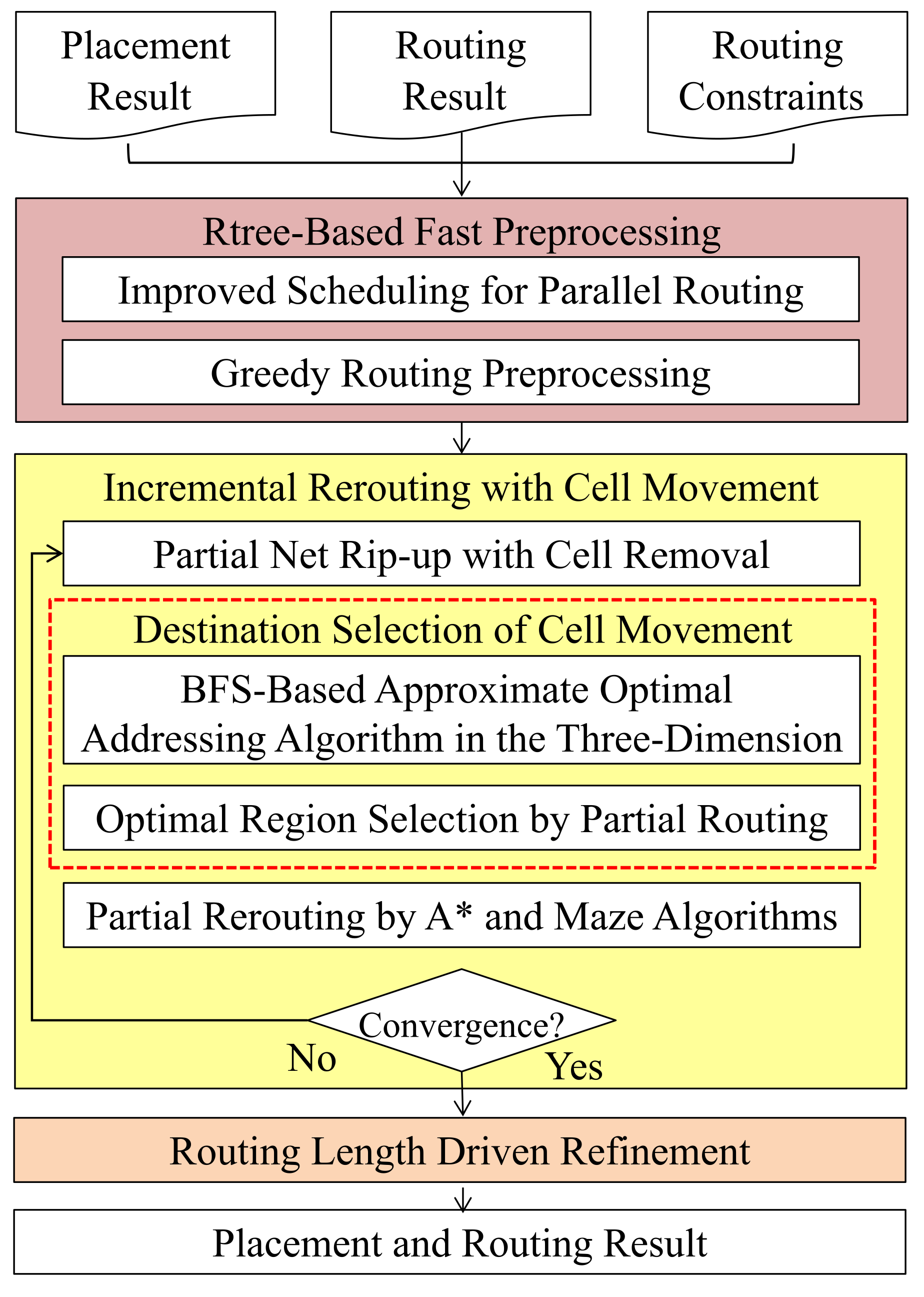
2.2. Our Algorithm Flow

Figure 1 shows the overall flow of the proposed approach, which consists of three major stages: Rtree-based fast preprocessing, incremental rerouting with cell movement, and routing length driven refinement. In the preprocessing stage, we first present improved scheduling for parallel routing based on R-tree. After that, a greedy selection strategy is used to accept the solution with routing length reduction. During the incremental rerouting with cell movement stage, four partial rip-up strategies are proposed to make a trade-off between quality and efficiency while removing the cell. According to different partial rip-up strategies, a BFS-based approximate optimal addressing algorithm in 3D and an optimal region selection by partial routing solution are proposed to find the candidate destinations of the removed cell. A partial rerouting algorithm hybrid A* and multi-source, multi-sink maze algorithm is proposed to find the optimal destination of cell movement in parallel. Finally, an efficient refinement is adopted to reduce the routing length further.

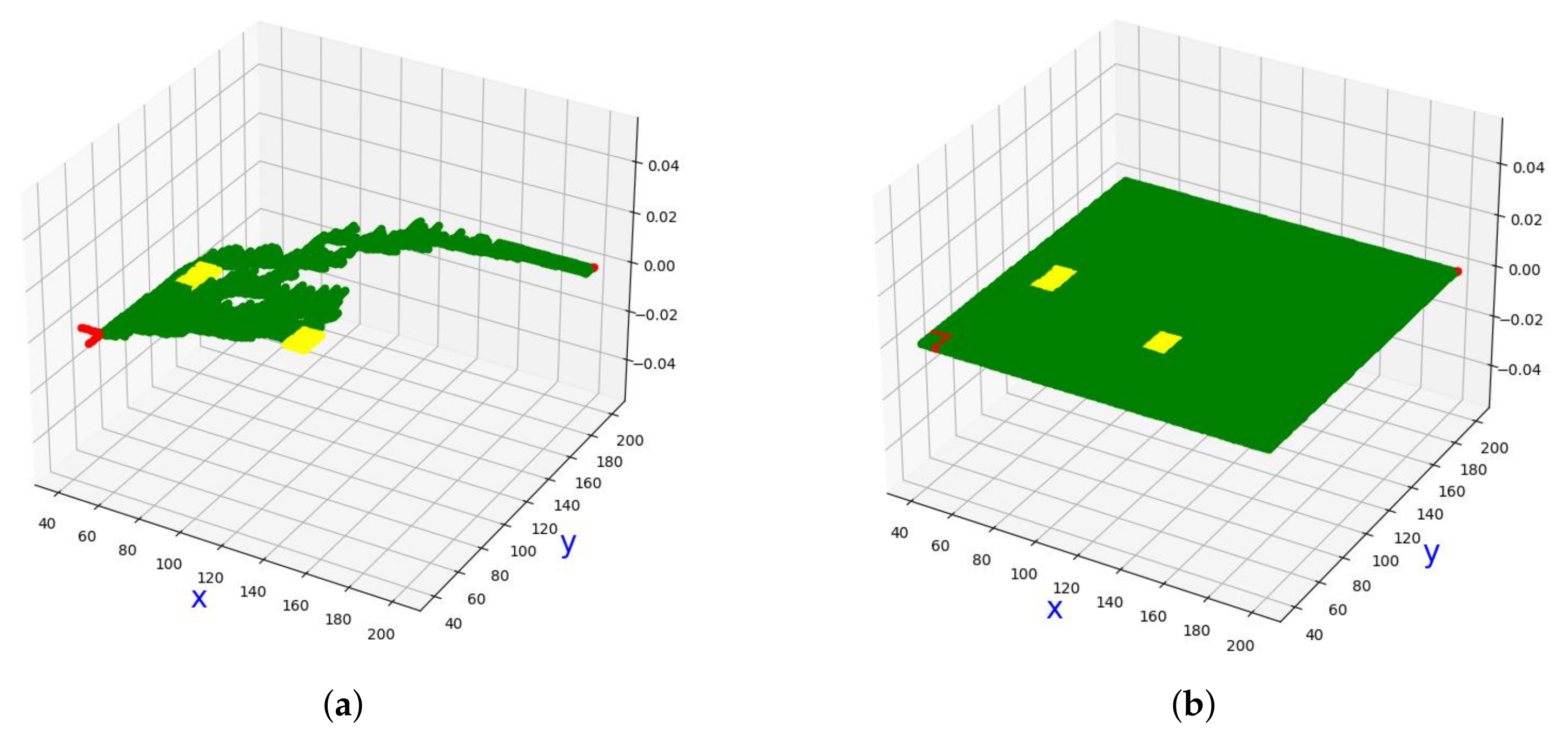
3. RTree-Based Fast Preprocessing

In the global routing stage, the complex net structure, unreasonable routing or infeasible ripping-up result in closed loops and needless nodes. The redundant routing result increases the routing length and makes the region congested. Firstly, we mark all the net points in the bounding box as unvisited, and the topology of the tree will be built in Figure 2a. A-F in Figure 2 are the grids where the net passes. Secondly, the depth-first search (DFS) technology is used to mark the visited nodes in Figure 2b, and the nodes that have no pin will be removed in the process of backtracking in Figure 2c,d. After the above operations, the closed loops of nets will be broken, and the redundant nodes will be deleted. More importantly, the routing length and congestion will be significantly improved.

According to the bounding boxes of the given initial routing result, we build R-trees [23] and later query nets with the disjoint border from the R-trees. Similar to [24], we propose the scheduling of all the batches in our work by Algorithm 1. Since conflicts are more likely to occur between large nets, line 1 sorts all nets in decreasing the size of the bounding boxes. Nets are assigned one after another by joining an existing batch or building a new batch (lines 2–18), thus minimizing the number of batches. R-trees are used to judge the overlap between a net bounding box and a candidate batch. In application, we found that most of the R-tree queries in the later stage of the original algorithm failed, which caused a lot of time to be wasted. Therefore, lines 9–11 added some criteria to judge whether enough nets have been added to a batch. Since nets with shorter wirelength have a smaller solution space and a larger number of pins makes it difficult to route, line 19 reordered the batchlist. In this way, the total scheduling runtime can be improved by 70× (detailed comparisons are shown in the Section 6.2). Figure 3 shows an example of our scheduling, where red and green rectangles represent different batches, respectively.

Algorithm 1 Improved Scheduling for Parallel Routing.

Input:  Nets; Output:  BatchList; 1: Sort all nets in decreasing size of the bounding boxes; 2: for each net $e_i$ do 3:   for each batch $b_j$ in BatchList do 4:    if batch $b_j$ is full then 5:     continue; 6:    end if 7:    if the bounding box of $e_i$ has no overlap with $b_j$ then 8:     Add $e_i$ into $b_j$; 9:     if $nums\left(b_j\right)\ge n_b$ or $A_{cur}/A_{total}>t$ then 10:      $b_j\leftarrow$ full; 11:     end if 12:     break; 13:    end if 14:    if $e_i$ has not been assigned to any batch then 15:     Build a new batch and added $e_i$; 16:    end if 17:   end for 18: end for 19: Sort the batchList with shorter wirelength and a larger number of pins.

Compared with the congestion-aware 3D global routing in the work [22], we use a greedy method of mixing FLUTE and maze routing in each batch to optimize the initial solution. Our greedy preprocessing algorithm for the initial global routing result is shown in Algorithm 2. Firstly, line 4 uses a very fast and accurate rectilinear Steiner minimal tree (RSMT) algorithm called fast lookup table estimation (FLUTE) [10]. A net-breaking technique is used for high-degree nets to reduce the net size until the table can be used. In addition, an edge shifting technique is used to direct routing demand away from the congested regions by moving some tree edges without increasing wirelength [25] in line 5. After that, all Steiner trees are broken into 2-pin nets, which are better results in 2D layout. Thus, we use L-shaped pattern routing and layer assignment to rapidly get a reasonable 3D routing result (lines 6–8). During multi-layer global routing, Ref. [26] adopted dynamic programming to find a layer assignment result such that the via cost is minimized while the given congestion constraints are satisfied. Lines 9–12 accept the result if the solution has no overflow and is shorter than the initial result. Otherwise, we use maze routing [25] to reroute the whole net in the 3D boundary. Maze routing is the most popular and powerful technique in global routing to find a path while avoiding congestion. According to some cost functions, maze routing facilitates the shortest path connecting two pins through the fewest congestion grids. The cost function will be introduced in Section 4.3.

Algorithm 2 Greedy Routing Preprocessing.

Input:  BatchList, Initial Global Routing; Output:  Routing Result; 1: for BatchList $b_j$ do 2:   for net $e_i$ in BatchList $b_j$ do 3:    Ripup initial routing solution; 4:    DoFLUTE; 5:    DoEdgeShift; 6:    for each sub-2-pin nets do 7:     Pattern routing and layer assignment; 8:    end for 9:    if !isOverflow $\&\&$ $r{l}_{So{l}_f}$ < $r{l}_{initial}$ then 10:     Accept the FLUTE solution $So{l}_f$; 11:     continue; 12:    end if 13:    Reject the FLUTE solution $So{l}_f$; 14:    Reroute with 3D maze routing; 15:    if $r{l}_{So{l}_m}$ > $r{l}_{initial}$ then 16:     Restore initial routing; 17:     continue; 18:    end if 19:    Accept the maze solution $So{l}_m$; 20:   end for 21: end for

4. Incremental Rerouting with Cell Movement

In this section, we introduce our partial rip-up, destination selection and partial rerouting algorithm. The specific process is as follows. Firstly, we calculate the wirelength of the bounding box that can be reduced by moving it to its optimal region [5], and reorder by the decreasing order. For each cell, we rip up the connected nets partially and find the candidate destinations. For each candidate destination, we first update the extra demand and check that there is no overflow constraint $C1$, and thus reroute the remaining routing paths and the destination gGrid to obtain the reduced routing length. Since, at most, only one destination will be selected, these rerouting processes can be processed in parallel.

4.1. Partial Net Rip-Up with Cell Removal

For cell movement, the nets which connect to the pins of removed cells relocated need to be ripped up before being re-routed. However, dismantling the entire net inevitably brings a lot of unnecessary recalculation because some parts of the nets are not directly connected with the pins of the removed cell or away from the congested region. It is time-saving and computation-reducing to retain some parts of the net which have little effect on the re-routing of the relocated cell. Therefore, under different conditions, we propose a novel method to achieve the different reuse of parts of routing paths which is suitable for our problem. This method is more comprehensive than the previous works [22] and SRP [19], where [22] would keep the remaining wires in one connected component and [19] do not consider the impact of the Steiner points. For convenience, we introduce these schemes in this section. When we delete the routing path connected to the pin on the cell to be moved, four cases will be considered as follows (the detailed illustration is shown in Figure 4). For simplicity, we only show the case of the 2D rip up. For a 3D case, the via above the minimum layer are treated as normal paths, and the via below the minimum layer may be removed as the pin is removed (the via which is used by other pins can be still reserved). Assuming that there are n nodes in the single net, by recursively traversing the nodes, we can dismantle the unwanted part of the net within $O\left(n\right)$ time complexity.

Case $R1$: In Figure 4a, grid (7, 3) contains two pins. After removing the red removed pin, we would not rip up any paths connecting to the grid, as in Figure 4b. If there is the minimum layer constraint on this net, and there is a via in this grid, only the via of another pin is reserved.

Case $R2$: In Figure 4c, grid (0, 3) only contains a removed pin, and we delete the connected paths from this pin until we reach a grid that contains a pin or a Steiner point, as in Figure 4d. In this case, the remaining paths may be divided into multiple subnets which are equal to the degree of this pin. We will connect these subnets and the relocated pin after finding the new location.

Case $R3$: In Figure 4e, grid (0, 3) contains a removed pin whose degree is larger than one. When the remaining path need to be connected (which is discussed in Section 4.2.1), we would not rip up any paths connecting to the grid, as in Figure 4f.

Case $R4$: In Figure 4g, grid (3, 0) contains a removed pin, and we delete the connected paths from this pin until reaching a grid that contains a pin or until the second passed Steiner point, as in Figure 4h. Compared with case $R2$, this case will destroy the local topology, and we believe that the construction of the first passed Steiner point will largely depend on the position of the removed pin. For example, if the removed pin is located at the grid (3, 4), the Steiner point in the grid (3, 3) would not guarantee the shortest length of the net.

4.2. Destination Selection of Cell Movement

In our work, we select one cell to remove each time, and find an optimal moving position to obtain the maximum routing length reduction. Different from the previous work [19], the purpose of SRP is to optimize routability. In this contest, we need to optimize the routing length as much as possible without causing routing overflow. In order to achieve this goal, we propose the following two candidate destination selection schemes.

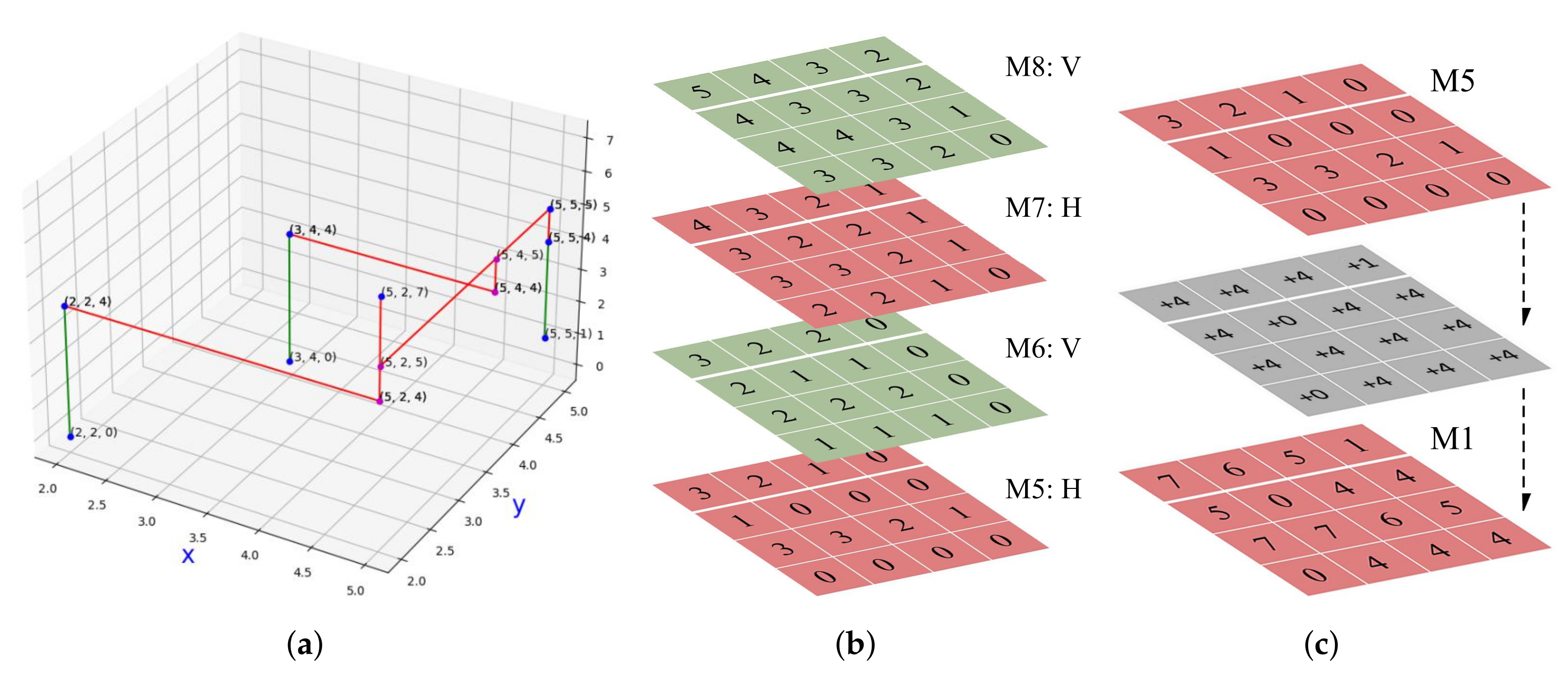
4.2.1. BFS-Based Approximate Optimal Addressing Algorithm in 3D

To reduce the number of routing operations, which is extremely time-consuming, we need to approximate the routing process as accurately as possible to select the destination. Based on some routing constraints (layer direction, minimum layer, via reused, overflow), we propose a breadth-first search (BFS)-based approximate optimal addressing algorithm in 3D in Algorithm 3. In this algorithm, we divide the routing range into two parts. The part on the minimum layer uses a 3D search strategy and directly performs calculations below the minimum layer to significantly reduce the number of search calculations.

Obviously, if the cell is moved beyond the outer border of its current routing paths, the routing length is almost impossible to reduce. The range $[x_l,y_b]\times [x_r,y_t]$ is obtained by the bounding box of all paths in the connected nets $E_i$. For each net $e_j\in E_i$, lines 5–9 first execute different rip-up strategies according to different situations to get the remaining paths. Since multiple subnets are searched together, it is challenging to ensure efficiency while considering the Steiner points. Therefore, if the net $e_j$ has another pin in the same grid $(x_i,y_i,z_{mi{n}_j})$ ($z_{mi{n}_j}$ denotes the pin coordinate in the z-direction on the minimum layer in net $e_j$), or the degree of this pin is greater than one, we need to ensure that each remaining path is still connected in this method (see Figure 4b,f). Otherwise, we delete the connected paths from this pin until reaching a grid that contains a pin or a Steiner point. Furthermore, line 10 calculates the routing length of the removed paths $r{l}_j$ and the removed via $\Delta vi{a}_{\{j,(x_i,y_i)\}}$, which has no overlap with other via in this net.

For each net $e_j$, the z-range $z_b,z_t$ is obtained by the bounding box of the z-direction of $e_j$ on the minimum layer where $z_t$ must larger than $z_b$ for the different layer directions (if the congestion is severe, we extend $z_t=z_t+1$). Lines 12–16 add the remaining paths to the queue q and mark them as visited, and the cost $di{s}_j$ of the gGrid p is 0. Lines 17–30 pop the gGrid in the queue one by one and search the adjacent gGrids according to the direction of the layer. If an adjacent gGrid is un-visited, mark it as visited and increase its cost by 1, and then add the gGrid to the queue except for the demand equal to the capacity (which means that no path can pass through this gGrid). Repeat the operation within the given search range $[x_l,y_b,z_b]\times [x_r,y_t,z_t]$ until the queue is empty. Finally, line 31 takes the cost of the layer $di{s}_{j,z_{mi{n}_j}}$ where the pin $z_{mi{n}_j}$ is located. Then, we add the length of the required via to each destination, and deduct the length of the overlapping part if the via of other pins can be reused. After searching for all the nets $E_i$, the cost $dis(x,y,z)$ represents the total routing length that the cell moves to the destination $(x,y,z)$, and $rl$ is the total rip-up routing length. Even if we consider the congestion area where a single net cannot pass through in lines 24–26, there may be multiple routing paths passing through the area close to overflow at the same time, which results in the actual routing length being larger than $dis(x,y,z)$. Therefore, when $dis(x,y,z)$ is less than $rl$, line 35 adds $grid(x,y,z)$ to the priority queue C.

Algorithm 3 The 3D BFS-based Approximate Optimal Addressing Algorithm.

Input: Removed cell i, the connected nets $E_i$, rip-up routing length $rl=0$; Output: Candidate destinations priority queue C; 1: $x_i,y_i\leftarrow$ the origin location of removed cell i; 2: $x_l,x_r\leftarrow$ the left, right border of all paths in nets $E_i$; 3: $y_b,y_t\leftarrow$ the bottom, top border of all paths in nets $E_i$; 4: for net $e_j\in E_i$ do 5:  if another pin in $grid(x_i,y_i,z_{mi{n}_j})$ or $degree>1$ then 6:   $ripupSe{t}_j$ ← keep all paths by $R1$ or $R3$; 7:  else 8:   $ripupSe{t}_j$ ← the remaining paths by $R2$; 9:  end if 10:  $rl\leftarrow rl+r{l}_j+\Delta vi{a}_{\{j,(x_i,y_i)\}}$; 11:  $z_b,z_t(>z_b)\leftarrow$ the bottom, top border of $e_j$ on the minimum layer $mi{n}_{l,j}$; 12:  for $p\in ripupSe{t}_j$ do 13:   $q.push\left(p\right)$; 14:   $visited\left(p\right)$ ← true; 15:   $di{s}_j\left(p\right)$ ← 0; 16:  end for 17:  while $q\ne ⌀$ do 18:   for $gri{d}_{cur}\in q$ do 19:    $gri{d}_{cur}.pop\left(\right)$; 20:    for $gri{d}_{adj}\in direction(gri{d}_{cur},z_{cur})$ do 21:     if $gri{d}_{adj}\in [x_l,y_b,z_b]\times [x_r,y_t,z_t]$ && $!visited\left(gri{d}_{adj}\right)$ then 22:      $visited\left(gri{d}_{adj}\right)\leftarrow true$; 23:      $di{s}_j\left(gri{d}_{adj}\right)\leftarrow di{s}_j\left(gri{d}_{cur}\right)+1$; 24:      if $d\left(gri{d}_{adj}\right)<c\left(gri{d}_{adj}\right)$ then 25:       $q.push\left(gri{d}_{adj}\right)$; 26:      end if 27:     end if 28:    end for 29:   end for 30:  end while 31:  $dis\leftarrow dis+di{s}_{j,z_{mi{n}_{l,j}}}+vi{a}_j-overlap(i,k_{k\in e_j\setminus i})$; 32: end for 33: for$(x,y,z)\in [x_l,y_b,z_b]\times [x_r,y_t,z_t]$do 34:  if $dis(x,y,z)<rl$ then 35:   Add $(x,y,z)$ to C; 36:  end if 37: end for

An example of this algorithm is shown in Figure 5. In the figure, we want to search for the candidate destination of the removed pin whose z-coordinate is $M1$ and minimum layer is $M5$ within the bounding box of the existing routing path. In Figure 5a, the red and green lines represent the routing path on the minimum layer and via, respectively. In our algorithm, we separate the routing region by minimum layer to improve efficiency. On the minimum layer, we set the routing paths in Figure 5a to 0, and use BFS to find the distance while the layer direction is satisfied in Figure 5b. After that, since the minimum layer constraint for the removed pin is $M5$, we take $M5$’s distance map and add the length of the required via to each gGrid in Figure 5c. In particular, when the via can be reused, only the length of the newly added non-overlapping part needs to be added. In this algorithm, each net in $E_i$ is unrelated and can be processed in parallel at the same time. In addition, dividing the search range according to the minimum layer can reduce a lot of search space, which makes the algorithm more efficient. Different from the distance formulation in the previous work [22], our direct search method is closer to the real routing process. Even though our method has spent more time than [22], a more accurate destination selection may reduce the time for subsequent reroutes.

Here we analyze the complexity of the algorithm. For each net $e_j$, there are $V=(x_l-x_r)\times (yt-yb)\times (z_t-z_b)$ gGrids in the search region. Lines 5–16 takes time $O\left(V\right)$. Each $pop$ and $push$ operation on the priority queue q takes time $O\left(lgV\right)$. For each gGrid, there are at most 4 neighbors adjacent to it. Lines 22–23 take time $O\left(1\right)$. Line 17 has at most V iterations for the whole loop. The total complexity is therefore $O\left(VlgV\right)$.

4.2.2. Optimal Region Selection Using Partial Routing Solution

In the previous section, due to the limitation of the search method, we require the remaining paths to be connected. This will cause the new destination of the cell to depend on the previous topological structure, and it is easy to fall into a locally optimal solution. In most cases, the structure of the first Steiner point directly connected to the removed cell is largely related to the cell location. Therefore, we adopt the $R4$ strategy, which deletes the connected paths from this pin until reaching a grid that contains a pin or the second passed Steiner point in the hope of constructing a better topology according to the new location of the cell. In this case, a net may be divided into multiple disconnected subnets. Therefore, we improve the optimal region technique in the previous work [5] to find the candidate destination of the cell.

In the previous work [5], if only one cell i is allowed to move, the region with the optimal wirelength after placing the cell is defined as the “optimal region” of this cell. This region is determined by the median idea in the work [27]. As shown in Figure 6a, we show the optimal region obtained by this method. For the movable cell i, we traverse all the connected nets and find their bounding boxes (not including this cell). For each net j, the left, right, lower and upper boundaries are denoted by $x_l,x_r,y_l,$ and $y_u$, respectively. In the figure, there are three nets connecting to cell i. There are 5, 4 and 3 cells (denoted by diamonds) in net 1, 2 and 3, respectively. The bold dotted boundary boxes are the bounding boxes for the nets excluding cell i. From [27], the optimal region $[x_{r_2},y_{l_2}]\times [x_{l_3},y_{u_2}]$ is given by the medians of the $x-$series $(x_{l_1},x_{l_2},x_{r_2},x_{l_3},x_{r_3},x_{r_1})$ and $y-$series $(y_{l_3},y_{u_3},y_{l_2},y_{u_2},y_{l_1},y_{u_2})$ of the bounding boxes. At any gGrid in this optimal region, the sum of the distances to the bold dotted boundary boxes is equal and smaller than the other gGrids.

In the previous work, the optimal region was only related to the cell’s position, and the minimum estimated wirelength may have a large gap with the actual routing length. In this work, we have identified the cell’s position as well as the actual routing solution. The information of routing paths usually contains routing constraints, such as layer direction and congestion. For example, in Figure 6b, we consider the routing paths on the basis of Figure 6a. In the figure, the straight line represents the remaining paths, and the dashed line represents the removed paths while removing cell i. In net 1, the cells at $y_{u_1}$ are routed downward instead of connected as a horizontal line because they are affected by the layer direction constraint. In this case, the optimal region is $[x_{r_2},y_{l_1}]\times [x_{l_3},y_{l_2}]$, which is smaller than the region in Figure 6a. The best moving destination of the removed cell are all $(x_{r_2},y_{l_2})$ in both two figures. Even in some complex situations, the original method may miss the correct location. In particular, we prioritize the gGrids such that the via can be reused in the optimal region. In general, this improved method can consider routing constraints as much as possible, and the runtime will not be increased while optimizing the results.

4.3. Partial Rerouting by A* and Maze Routing Algorithms

A complete routing tree is built by re-routing the several disconnected sub-nets together. Before proposing the routing algorithm, we first give our cost function and briefly explain some basic routing operations in our algorithm. In our problem, the via is simplified to route on the z-direction. Thus, the cost function presented in the work [9] is shown as follows:

$$cos{t}_1\left(u\right)=wl\left(u\right)+wl\left(u\right)\times \frac{d\left(u\right)}{c\left(u\right)}\times \alpha \times \frac{1}{1+e^{\beta \times r\left(u\right)}},$$

(1)

where $wl\left(u\right)$ is the wirelength cost, and the function on the right side forms the congestion cost. $d\left(u\right)/c\left(u\right)$ and $r\left(u\right)$ represent the possibility of overflow and the resource, respectively. $\alpha$ determines the ratio of the congestion term, and variable $\beta$ of the logistic function determines the global router’s sensitivity to overflow. In this problem, there is already a legal initial routing solution, and the objective of rerouting is to reduce the routing length without causing routing overflow. In order to make the solution easier, we use multiple iterations for routing every time until we get a solution without overflow. The cost function in our work is modified as follows:

$$cos{t}_2\left(u\right)=1+\frac{\alpha }{1+e^{\beta \times r\left(u\right)}}+iter\times max(\theta -r\left(u\right),0)\times \gamma ,$$

(2)

where $iter\in \{1,2,3\}$ is the iteration in the routing process and $\gamma$ is a penalty factor to avoid routing through the gGrid that is about to overflow. $\theta$ is a positive integer that controls the available capacity. We remove $d\left(u\right)/c\left(u\right)$ because none of the grids overflowed (must be $d\left(u\right)\le c\left(u\right)$) in this problem. To reduce the routing length as much as possible, we should not treat gGrids differently as long as there are sufficient resources. We only need to avoid crossing the gGrid where the demand is close to capacity.

To avoid unnecessary searches, we only rerouted inside the bounding box that the origin routing path of the net passed through at the beginning. Since the pins are usually on the lower layer, the higher metal layers are usually not used for 3D routing. Therefore, the congestion of the lower layers would be greater than that of the higher layers. If a solution without overflow can be found, we expand the search range in the z-direction as the iteration increases. We do not expand in the $x,y$-direction because we prefer to route with less congestion when the same routing length would be increased.

Among the current global routing tools, the more popular one is maze routing with multiple sources and multiple sinks. In this problem, the goal is to connect the removed cell and multiple subnets (in most cases, no more than 3). We use multi-source multi-sink maze routing [25] to generate good routing solutions for the multi-pin nets. The time complexity is $O\left(VlogV\right)$, where V is the gGrid points in the search region. This method considers the existing routing tree instead of restricting the two endpoints of the routing path to be the original endpoints of the edge being routed. We treat the removed cell as the source, and all the gGrid points on the remaining paths as sinks. Similar to Dijkstra’s algorithm, when a gGrid point is extracted from the priority queue, the cost is the shortest distance from sources to this gGrid point. Once a gGrid point in a sink is extracted from the priority queue, new sources are constructed together with old sources, the shortest paths, and the encountered subnets. The search process is performed again until all the gGrid points are connected.

However, in our work, the difference is that we only partially rip up the net. For example, we adopt the $R2$ rip up strategy to reroute the candidate destinations obtained in Section 4.2.1 (the worst case is to connect the disconnected subnets according to the $R3$ situation, and then connect to the target gGrid. Therefore, it will be better than the estimated result); for the candidate destinations obtained in Section 4.2.2, the $R4$ rip up strategy is adopted to reroute. For the case where a cell will connect to a subnet, we can use the A* algorithm [28] to improve efficiency. The A* algorithm has been applied to global routing [29]. The A* algorithm is the most effective direct search method for solving the shortest path in a static road network, and it is also a practical algorithm for solving many search problems. If the estimated distance value is closer to the actual value in the algorithm, the search speed is faster. In our method, we use the priority queue to select the gGrid $(x,y,z)$ with the current lowest cost, and then use the following heuristic function $Cos{t}_{astar}$ (3) to guide the search direction of the algorithm:

$$Cos{t}_{astar}=Cos{t}_{predict}+(Cos{t}_{cur}+Cos{t}_{step}(x,y,z)),$$

(3)

where $Cos{t}_{predict}$, $Cos{t}_{cur}$ and $Cos{t}_{step}(x,y,z)$ represent the minimum cost estimate to the target gGrid, current cost, and the step cost with the current gGrid to the next gGrid, respectively. If $Cos{t}_{predict}$ is smaller than the actual routing length, the optimal solution can be obtained while the search range is large and the efficiency is low. If $Cos{t}_{predict}$ is equal to the actual routing length, the search efficiency at this time is the highest, and the solution is optimal. The $Cos{t}_{predict}$ is estimated by 3D distance estimation. In the x and y direction, the distance estimation is carried out by the Manhattan distance between the current gGrid and the target gGrid. In the z direction, the distance is estimated by the following equation.

$$\left\{\begin{array}{c}abs(z_{cur}-z_{tar}),z_{cur}\ne z_{tar},\hfill \\ 0,z_{cur}=z_{tar}\&y_{cur}=y_{tar}\&\mathrm{direction}\mathrm{is}\mathrm{horizontal},\hfill \\ 0,z_{cur}=z_{tar}\&x_{cur}=x_{tar}\&\mathrm{direction}\mathrm{is}\mathrm{vertical},\hfill \\ 2,\mathrm{else}.\hfill \end{array}\right.$$

(4)

The result estimated is the minimum routing result that satisfies the layer direction constraint, which must be no greater than the actual routing result. Therefore, while ensuring the quality of the solution, it can ensure that the search is carried out in the direction of the target point, which is obviously better than the directionless search of Dijkstra’s algorithm. A simple illustration of the 2D routing process is shown in Figure 7, which is similar when extended to 3D. In the figure, red points represent the subnet and the removed pin to be connected, yellow rectangles are obstacles where demand is equal to capacity, and green points represent the grid traversed during the search process. In our algorithm, we control the search range within the bounding box of the existing paths. Different from the complete search of Dijkstra’s algorithm in Figure 7b, the A* algorithm is directional, which can reduce a large number of unnecessary searches, as in Figure 7a.

5. Routing Length Driven Refinement

When the number of movable cells reaches the prescribed maximum number, we stop looking for the cells that need to be moved. However, due to the movement sequence, some cells that have already moved can be optimized again. In addition, due to the partial rip-up and reroute of the net in the above section, some of the nets may not have the optimal topology. Therefore, in this section, we further optimize the results. In this stage, $\theta$ in Equation (2) is equal to one, using all capacity as much as possible.

If a cell that has been moved is encountered, it will move again. Therefore, we propose a similar but faster 2D BFS scheme to move the cell in this section. Similar to the process of Algorithm 3, we ignore some routing constraints and perform a breadth-first search in a 2D range. The distance of the $z-$direction is replaced by the minimum distance between the subnet and the removed pin. If these are on the same layer and not on the same straight line, the distance in the $z-$direction is 2. After considering the reuse of the vias, the estimated distance for the cell to move to any point in the range is obtained. Since this strategy ignores some routing constraints, the obtained candidate locations will be slightly more than the 3D search. At this stage, there are fewer destinations where the cell can move with the reducing routing length. We adopt the $R4$ rip-up method and set the termination condition of rerouting as long as there is a location that the length can be reduced.

After that, we reroute each net to get a better topology, as in Algorithm 4. In the algorithm, line 4 first reroutes with the FLUTE, which is shown in Algorithm 2, lines 4–8. If the number of pins does not exceed 9, FLUTE usually find the optimal solution. Otherwise, even if the FLUTE solution $So{l}_f$ can achieve a smaller length than the initial solution, we still use maze routing to get a solution $So{l}_m$. In lines 14–18, when the minimum length of these two solutions is larger than the initial solution, we restore the initial routing state. Otherwise, we choose the solution which has a smaller routing length. It should be noted that when the rerouted is unsuccessful or the solution has routing overflow, the routing length $rl$ is set to be INT_MAX.

Algorithm 4 Routing Length Driven Refinement.

Input:  BatchList, Global Routing Result; Output:  Final Routing Result; 1: for BatchList $b_j$ do 2:   for net $e_i$ in BatchList $b_j$ do 3:    Rip-up routing solution; 4:    FLUTE in Algorithm 2, lines 4–8; 5:    if $r{l}_{So{l}_f}$ ≤ $r{l}_{initial}$ then 6:     if $pins.size\left(\right)\le 9$ then 7:      Accept the FLUTE solution $So{l}_f$; 8:      continue; 9:     else 10:      Store the FLUTE solution $So{l}_f$; 11:     end if 12:    end if 13:    Reroute the solution $So{l}_m$ with 3D maze routing; 14:    if $min(r{l}_{So{l}_f},r{l}_{So{l}_m})$ > $r{l}_{initial}$ then 15:     Restore initial routing; 16:    else 17:     Accept new solution by $min(r{l}_{So{l}_f},r{l}_{So{l}_m})$; 18:    end if 19:   end for 20: end for

6. Experimental Results

In this section, we first introduce our experimental setup and benchmarks. Then, we study the parallel technology used in this paper to show its impact on performance. After that, we compare our results with the top 3 winners of the ICCAD’20 CAD contest. Finally, we change the maximum cell movement constraint to demonstrate the performance of our proposed algorithm further.

6.1. Experimental Setup and Benchmarks

We implemented our routing with the cell movement algorithm in the C++ programming language on a 64-bit CentOS Linux workstation with an Intel(R) Xeon(R) CPU [email protected] GHz, 128 GB memory, and 8 threads. All the experiments were based on the benchmark suite of the CAD contest benchmarks from ICCAD 2020 [30].

Table 1. Benchmark statistics.

Case	#gGrids	#Layers	#CellInsts	#Nets	Initial #Routes	Initial Length	Max Move
case1	5 × 5	3	8	6	42	64	2
case2	4 × 4	3	6	6	20	30	3
case3	27 × 33	7	2735	2644	26,046	32,600	820
case4	277 × 277	12	204,206	179,996	3,530,382	4,680,681	61,261
case5	104 × 103	16	96,682	92,546	1,404,555	1,763,627	29,004
case6	237 × 236	16	352,269	332,080	4,575,644	7,188,481	105,680
case3B	29 × 29	7	2604	2563	24,829	29,748	781
case4B	277 × 277	12	207,347	183,137	3,661,438	4,886,698	62,204
case5B	104 × 103	16	96,689	92,559	1,368,552	1,721,530	29,006
case6B	237 × 236	16	352,234	332,045	4,685,372	7,340,802	105,670

shows the statistics of the released benchmarks, where “#gGrids”, “#Layers”, “#CellInsts”, “#Nets”, and “Initial #Routes” represent the number of gGrids, routing layers, cells, nets, and the initial routes, respectively. “Initial Length” denotes the total routing length of the initial routes. “Max Move” is the maximum cell movement constraint, which is limited to 30% among all cells in the contest. In these benchmarks, the scales of case1 and case2 are too small and are only used as initial examples in the contest, so that subsequent experiments will exclude these two examples.

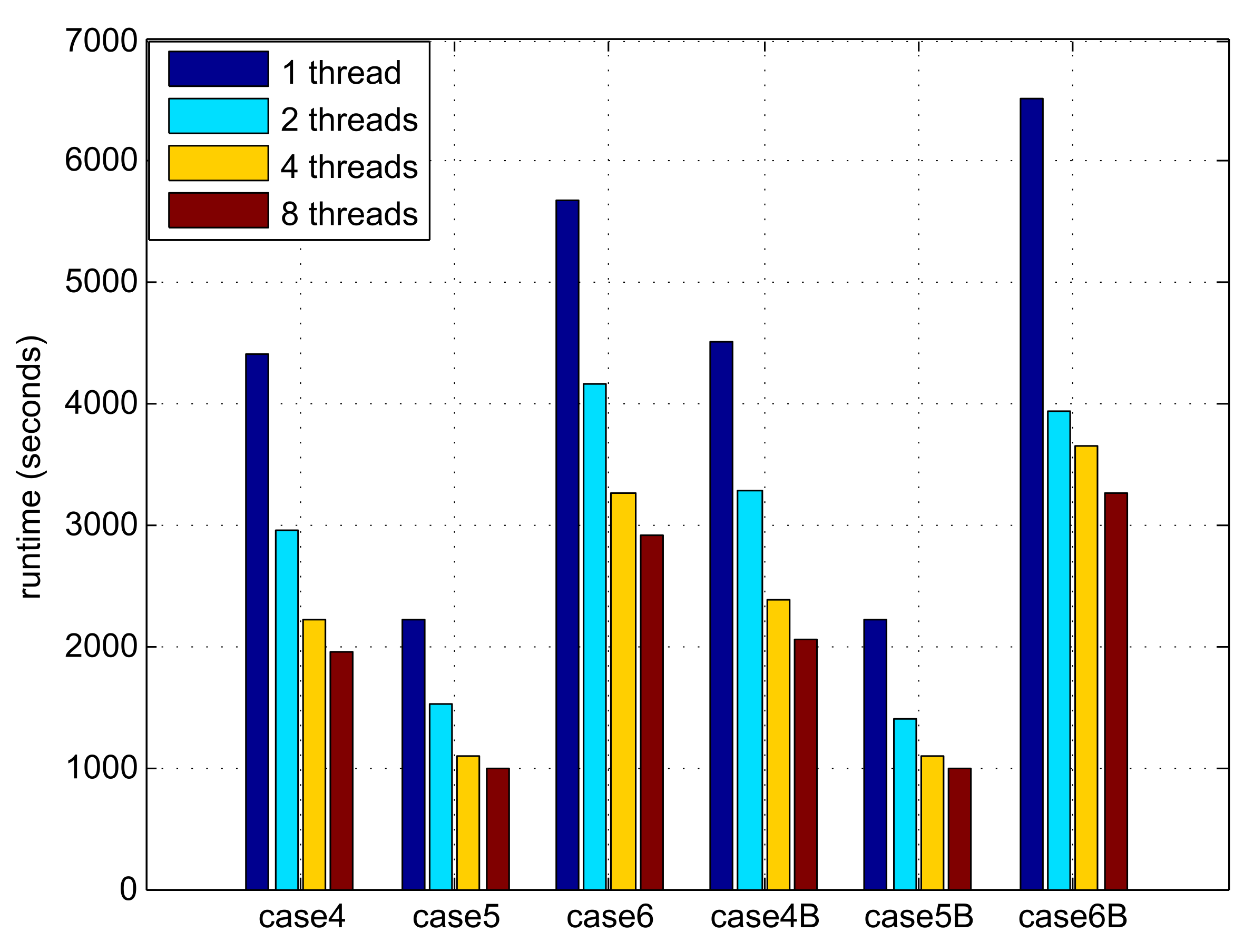
6.2. Parallel Technology

In this subsection, we study the parallel technology used in this paper to show its impact on performance. Firstly, we show the comparison results of the simultaneous maze rerouting for all nets with the batch scheduling strategy in

Table 2. Comparison results with the batch scheduling strategy.

Case	No Parallel		Batch Scheduling [24]			Improved Batch Scheduling
	RL-Red.	R-Times	B-Times	RL-Red.	R-Times	B-Times	RL-Red.	R-Times
case4	1,614,410	85	11.81	1,614,207	31	0.19	1,614,468	23
case5	442,207	25	7.94	441,314	18	0.13	441,678	15
case6	2,311,638	324	62.24	2,301,046	161	0.61	2,307,982	106
case4B	1,678,151	79	13.13	1,677,705	39	0.23	1,678,086	27
case5B	424,909	24	7.73	424,220	20	0.13	424,626	16
case6B	2,348,845	352	62.87	2,325,592	187	0.66	2,339,623	121
Normalized	1.001	2.629	73.044	0.998	1.391	1.000	1.000	1.000

. In the table, “RL-Red.”, “B-Times”, and “R-Times” denote the routing length reduction, the batch scheduling runtime (seconds), and the routing runtime (seconds), respectively. The difference between the improved batch scheduling and the original method in [24] is shown in Algorithm 1, line 9, where $n_b,t$ would be chosen by 24 and 0.5. On average, our parallel rerouting can achieve $2.629\times$ faster routing runtime compared with the serial rerouting, and the improved batch scheduling strategy speeds up the origin process by $73\times$. As the number of nets in each batch increases, the routing length decreases because the ordering of nets is destroyed, which also reduces the routing efficiency.

In Section 4.2.1, we proposed a 3D, BFS-based approximate optimal addressing algorithm to find the candidate destinations for the relocated cell. According to the minimum layer constraint, the space is divided into upper and lower parts in our algorithm. The upper part uses the search strategy, and the lower part is directly calculated. In addition, we assume that each net is not related to each other, so it can be parallelized. In Figure 8, “M1” represents the method of directly searching for the layer where the pin is located, and “M2” represents our algorithm. In the figure, we can see that the parallel operation of the connected nets can reduce the running time by about half. In addition, our method can achieve different degrees of efficiency improvement according to the proportion of the minimum layer which occupies the layers that the net passes through. This method of dividing the routing range into two parts according to the minimum layer constraint is also applied to our routing algorithm.

In Section 4.2, the routing length reduction by each cell move is more significant in the early iterations, which also means that there are a large number of candidate destinations. Therefore, we select at most the first $n_s$ candidate destinations with lower cost. For example, we will get a priority queue that estimates the routing length reduction in the 3D BFS-based approximate optimal addressing algorithm. Only gGrids with costs greater than 0 will be added to this priority queue. If the number is greater than $n_s$, only the first $n_s$ items will be taken. In the optimal region selection algorithm, if the number of optimal regions is greater than $n_s$, we give priority to locations where the vias can be reused or have enough $r\left(u\right)$. This method is similar to the top-k candidate positions in work [22]; the difference is that our available candidate destinations may be less than $n_s$. To obtain the trade-off between solution quality and runtime, we set $n_s$ as 8/16, as the number of gGrids is larger/less than 40,000 in this work. These $n_s$ destinations can be rerouted in parallel, and finally, the destination with maximum routing length reduction is selected.

In the entire algorithm, the more time-consuming operations mainly include preprocessing, rip-up, destination selection, partial rerouting for routing length estimation, restoration (routing length is not reduced)/actual routing (routing length reduction), and refinement. Parallel technology can be used in some operations, but there are still certain bottlenecks. For example, in preprocessing and refinement, it is possible to divide the area and thus perform rerouting simultaneously, but it is difficult for the large nets that occupy the primary rerouting time to be independent of each other. In the destinations selection, we can search for different nets simultaneously. However, the number of nets connected to each cell is usually not very large, and the time is mainly affected by the nets with the most search layers in the z-direction. In partial rerouting for routing length estimation, compared with the number of threads, the candidate gGrids are not too numerous, and this value will continue to decrease as the number of moved cells increases. Therefore, the time mainly depends on the gGrid with the longest rerouting time. Combining the above-mentioned technologies, we show the impact of our parallel technology on performance in Figure 9. As the result, our proposed algorithm can obtain an average speedup of $2.15\times$ by using 8 threads.

6.3. Comparison of Results with the Top Three Winners

To demonstrate the performance of our proposed algorithm, we compared it with the top 3 winners of the 2020 ICCAD CAD contest [21]. In this contest, the evaluation score is calculated by summating the routing length reduction of all the nets. The ranking of this contest is based on the summation of the score, while the runtime is limited to 1 h for each case.

Table 3. Comparison of the total length reduction and runtime between our algorithm and top three winners.

Case	First Place		Second Place		Third Place		Ours
	RL-Red.	Times	RL-Red.	Times	RL-Red.	Times	RL-Red.	Times
case3	11,425	34	11,428	4	11,557	111	11,574	24
case4	2,046,811	2221	2,048,105	804	2,037,598	3441	2,064,165	1952
case5	695,219	903	685,173	183	682,963	1213	695,344	999
case6	2,721,274	3171	2,687,926	2217	2,656,320	3511	2,737,732	2918
case3B	11,237	31	11,073	4	11,289	206	11,309	18
case4B	2,182,574	2299	2,180,172	786	2,167,411	3371	2,196,644	2050
case5B	664,347	886	654,797	237	654,183	1226	664,440	989
case6B	2,748,097	3406	2,722,222	2801	2,668,052	3514	2,787,052	3265
Normalized	0.993	1.160	0.985	0.402	0.983	2.986	1.000	1.000

shows the comparison results of the total routing length reduction and runtime between our algorithm and the top three winners. In the table, “RL-Red.”, “Times”, and “Normalized” represent the routing length reduction, runtime for seconds, and the normalized ratios based on our algorithm. The best result for each benchmark is marked in bold. As shown in the table, our algorithm has achieved the best results in all released benchmarks. On average, our algorithm demonstrates improvements of 0.7%, 1.5%, and 1.7% for the first, second, and third place with the comparable runtime, respectively.

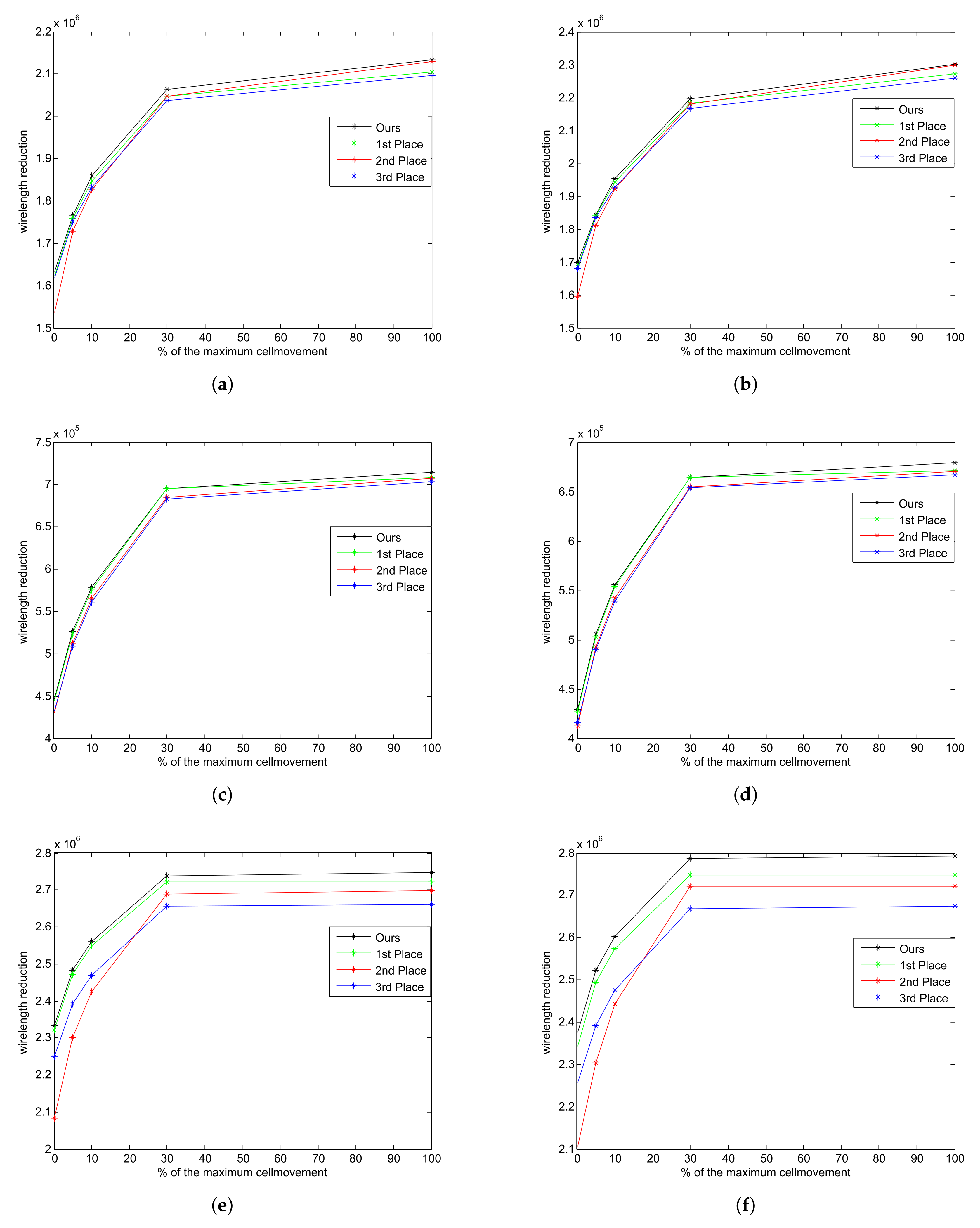
6.4. Results with Relaxed Max Cell Movement Constraint

In this contest, most of the constraints are hard constraints; that is, a legal routing result cannot be produced if they are violated. In practical applications, the maximum cell movement constraint $C3$ may not be necessarily limited by 30%. The 2020 ICCAD contest also gives a reduced routing length by changing the limited maximum cell movement to 0%, 5%, 10%, 30%, and 100%, respectively. Since the contest does not report runtime, we compare the routing length reduction in Figure 10 while the runtime of our results is satisfied within a 1 h limitation. The black, green, red, and blue colored lines in the figure represent our method and the top three winners, respectively. The horizontal axis is the different percentage of maximum cell movement, and the vertical axis is the routing length reduction. As can be seen from the figure, the black line representing our method is always at the top among all lines. This not only illustrates the effectiveness of our routing algorithm but also our cell movement strategy.

7. Conclusions

To resolve the conservative margin reservation and the mis-correlation problem in the divide-and-conquer place and route approach, we design an effective and efficient algorithm to co-optimize the detailed placement and global routing with complex routing constraints. A fast preprocessing technology based on R-tree is presented to improve the initial routing results. During destination selection of cell movement, we propose a 3D, BFS-based approximate optimal addressing algorithm and an optimal region selection using the partial routing solution to find the required locations. A hybrid A* and multi-source, multi-sink maze rerouting algorithm is proposed to find the final destination of cell movement in parallel. The experimental results show that we can obtain the best results with any maximum cell movement. Furthermore, with more advanced manufacturing processes, the constraints continue to increase, such as voltage area constraints, R/C characteristics in different layers, and the timing-based net weight. Our proposed algorithm can be effectively extended to address these problems.

References

1. Alpert, C.J.; Mehta, D.P.; Sapatnekar, S.S. Handbook of Algorithm for Physical Design Automation; Auerbach Publications: New York, NY, USA, 2008. [Google Scholar]
2. Kim, M.C.; Viswanathan, N.; Li, Z.; Alpert, C. ICCAD-2013 CAD contest in placement finishing and benchmark suite. In Proceedings of the IEEE/ACM International Conference on Computer-Aided Design, San Jose, CA, USA, 18–21 November 2013. [Google Scholar]
3. Caldwell, A.E.; Kahng, A.B.; Markov, I.L. Optimal partitioners and end-case placers for standard-cell layout. IEEE Trans. Comput.-Aided Des. Integr. Circuits Syst. 2000, 19, 1304–1313. [Google Scholar] [CrossRef]
4. Chen, T.C.; Jiang, Z.W.; Hsu, T.C.; Chen, H.C.; Chang, Y.W. NTUplace3: An analytical placer for large-scale mixed-size designs with preplaced blocks and density constraints. IEEE Trans. Comput.-Aided Des. Integr. Circuits Syst. 2008, 27, 1228–1240. [Google Scholar] [CrossRef] [Green Version]
5. Pan, M.; Viswanathan, N.; Chu, C. An efficient and effective detailed placement algorithm. In Proceedings of the IEEE/ACM International Conference on Computer-Aided Design, San Jose, CA, USA, 6–10 November 2005; pp. 48–55. [Google Scholar]
6. Chow, W.K.; Kuang, J.; He, X.; Cai, W.; Young, E.F. Cell Density-Driven Detailed Placement with Displacement Constraint. In Proceedings of the 2014 on International Symposium on Physical Design, Petaluma, CA, USA, 30 March–2 April 2014. [Google Scholar]
7. Roy, J.A.; Markov, I.L. High-performance routing at the nanometer scale. IEEE Trans. Comput.-Aided Des. Integr. Circuits Syst. 2008, 27, 1066–1077. [Google Scholar]
8. Wu, T.H.; Davoodi, A.; Linderoth, J.T. Grip: Scalable 3d global routing using integer programming. In Proceedings of the 46th Annual Design Automation Conference, San Francisco, CA, USA, 26–31 July 2009. [Google Scholar]
9. Liu, J.; Pui, C.W.; Wang, F.; Young, E.F.Y. Cugr: Detailed-routability-driven 3d global routing with probabilistic resource model. In Proceedings of the 2020 57th ACM/IEEE Design Automation Conference (DAC), San Francisco, CA, USA, 20–24 July 2020. [Google Scholar]
10. Chu, C.; Wong, Y.C. Flute: Fast lookup table based rectilinear steiner minimal tree algorithm for vlsi design. IEEE Trans. Comput.-Aided Des. Integr. Circuits Syst. 2007, 27, 70–83. [Google Scholar] [CrossRef]
11. Liu, W.H.; Kao, W.C.; Li, Y.L.; Chao, K.Y. Nctu-gr 2.0: Multithreaded collision-aware global routing with bounded-length maze routing. IEEE Trans. Comput.-Aided Des. Integr. Circuits Syst. 2013, 32, 709–722. [Google Scholar]
12. Xu, Y.; Zhang, Y.; Chu, C. Fastroute 4.0: Global router with efficient via minimization. In Proceedings of the Asia and South Pacific Design Automation Conference (ASP-DAC), Yokohama, Japan, 19–22 January 2009. [Google Scholar]
13. Chen, H.Y.; Hsu, C.H.; Chang, Y.W. High-performance global routing with fast overflow reduction. In Proceedings of the ACM/IEEE Design Automation Conference (DAC), Yokohama, Japan, 19–22 January 2009. [Google Scholar]
14. Chang, Y.J.; Lee, Y.T.; Wang, T.C. Nthu-route 2.0: A fast and stable global router. In Proceedings of the IEEE/ACM International Conference on Computer-Aided Design (ICCAD), San Jose, CA, USA, 10–13 November 2008. [Google Scholar]
15. Pan, M.; Chu, C. IPR: An integrated placement and routing algorithm. In Proceedings of the ACM/IEEE Design Automation Conference (DAC), San Diego, CA, USA, 4–8 June 2007. [Google Scholar]
16. Dai, K.R.; Lu, C.H.; Li, Y.L. GRPlacer: Improving routability and wire-length of global routing with circuit replacement. In Proceedings of the IEEE/ACM International Conference on Computer-Aided Design (ICCAD), San Jose, CA, USA, 2–5 November 2009. [Google Scholar]
17. Roy, J.A.; Viswanathan, N.; Nam, G.J.; Alpert, C.J.; Markov, I.L. CRISP: Congestion reduction by iterated spreading during placement. In Proceedings of the IEEE/ACM International Conference on Computer-Aided Design (ICCAD), San Jose, CA, USA, 2–5 November 2009. [Google Scholar]
18. Pan, M.; Chu, C. FastRoute: A Step to Integrate Global Routing into Placement. In Proceedings of the IEEE/ACM International Conference on Computer-Aided Design (ICCAD), San Jose, CA, USA, 5–9 November 2006. [Google Scholar]
19. He, X.; Chow, W.K.; Young, E.F. SRP: Simultaneous routing and placement for congestion refinement. In Proceedings of the ACM International Symposium on Physical design (ISPD), Stateline, NV, USA, 24–27 March 2013; pp. 108–113. [Google Scholar]
20. Fontana, T.A.; Aghaeekiasaraee, E.; Netto, R.; Almeida, S.F.; Gandhi, U.; Tabrizi, A.F.; Westwick, D.; Behjat, L.; Güntzel, J.L. ILP-Based Global Routing Optimization with Cell Movements. In Proceedings of the IEEE Computer Society Annual Symposium on VLSI (ISVLSI), Tampa, FL, USA, 7–9 July 2021. [Google Scholar]
21. Hu, K.S.; Yang, M.J.; Yu, T.C.; Chen, G.C. ICCAD-2020 CAD contest in Routing with Cell Movement. In Proceedings of the IEEE/ACM International Conference on Computer-Aided Design, San Diego, CA, USA, 2–5 November 2020. [Google Scholar]
22. Zou, P.; Lin, Z.; Ma, C.; Yu, J.; Chen, J. Late Breaking Results: Incremental 3D Global Routing Considering Cell Movement. In Proceedings of the 2021 58th ACM/IEEE Design Automation Conference (DAC), San Francisco, CA, USA, 5–9 December 2021; pp. 1366–1367. [Google Scholar]
23. Guttman, A. R-trees: A dynamic index structure for spatial searching. In Proceedings of the 1984 ACM SIGMOD international Conference on Management of Data, Boston, MA, USA, 18–21 June 1984; pp. 47–57. [Google Scholar]
24. Chen, G.; Pui, C.W.; Li, H.; Young, E.F.Y. CU: Detailed Routing by Sparse Grid Graph and Minimum-Area-Captured Path Search. IEEE Trans. Comput.-Aided Des. Integr. Circuits Syst. 2020, 39, 1902–1915. [Google Scholar] [CrossRef]
25. Pan, M.; Chu, C. FastRoute 2.0: A High-quality and Efficient Global Router. In Proceedings of the 2007 Asia and South Pacific Design Automation Conference, Yokohama, Japan, 23–26 January 2007. [Google Scholar]
26. Lee, T.H.; Wang, T.C. Congestion-Constrained Layer Assignment for Via Minimization in Global Routing. IEEE Trans. Comput.-Aided Des. Integr. Circuits Syst. 2008, 27, 1643–1656. [Google Scholar]
27. Goto, S. An Efficient Algorithm for the Two-Dimensional Placement Problem in Electrical Circuit Layout. IEEE Trans. Circuits Syst. 1981, CAS-28, 12–18. [Google Scholar] [CrossRef]
28. Hart, P.E.; Nilsson, N.J.; Raphael, B. A formal basis for the heuristic determination of minimum cost paths. IEEE Trans. Syst. Sci. Cybern. 1968, SSC-4, 100–107. [Google Scholar] [CrossRef]
29. Clow, G.W. A global routing algorithm for general cells. In Proceedings of the ACM/IEEE 21st Design Automation Conference, Albuquerque, NM, USA, 25–27 June 1984. [Google Scholar]
30. 2020 CAD Contest at ICCAD on Routing with Cell Movement. Available online: http://iccad-contest.org/2020/problems.html (accessed on 1 November 2021).
Figure 1. Our proposed algorithm.
Electronics 11 00051 g001
Figure 2. An example of closed loops and redundant nodes being removed based on depth-first search. (a) Mark all the net points in the bounding box as unvisited. (b) Mark the visited nodes by the DFS technology. (c,d) The nodes that have no pin will be removed in the process of backtracking.
Electronics 11 00051 g002
Figure 3. An example of scheduling, where red and green rectangles represent different batches.
Electronics 11 00051 g003
Figure 4. Four rip up cases considered in our flow. The diamond and circle represent the pin and the Steiner point, respectively. The pin to be removed is marked in red, and the grid in the lower left corner is (0, 0). (a) Grid (7, 3) contains a removed pin. (b) The remaining path and pin for the case R 1 . (c) Grid (0, 3) contains a removed pin. (d) Delete paths until reaching a grid that contains a pin or a Steiner point for the case R 2 . (e) Grid (0, 3) contains a removed pin whose degree is two. (f) Ensure the connectivity of the remaining path for the case R 3 . (g) Grid (3, 0) contains a removed pin. (h) The remaining path after rip up for the case R 4 .
Electronics 11 00051 g004
Figure 5. An example of 3D BFS search process in Algorithm 3. The z-coordinate of the removed pin is M 1 and its minimum layer is M 5 . (a) Routing paths of a net, where the red and green lines represent the routing path on the minimum layer and via, respectively. (b) The distance map above the minimum layer, where the red layer direction is horizontal and the green layer direction is vertical. (c) The distance map of layer M 1 is directly calculated from the distance map of the minimum layer.
Electronics 11 00051 g005
Figure 6. The optimal region obtained by: (a) the method presented in the work [5]. (b) the improved method in our work.
Electronics 11 00051 g006
Figure 7. The search process of (a) the A* algorithm; (b) Dijkstra’s algorithm.
Electronics 11 00051 g007
Figure 8. Comparisons of the 3D, BFS-based approximate optimal addressing algorithm comparisons.
Electronics 11 00051 g008
Figure 9. Runtime comparison among 1, 2, 4 and 8 threads.
Electronics 11 00051 g009
Figure 10. Experimental results with relaxed max cell movement constraint. (a) Case4. (b) Case4b. (c) Case5. (d) Case5b. (e) Case6. (f) Case6b.
Electronics 11 00051 g010