On Performance of Sparse Fast Fourier Transform Algorithms Using the Aliasing Filter

Abstract

Computing the sparse fast Fourier transform (sFFT) has emerged as a critical topic for a long time because of its high efficiency and wide practicability. More than twenty different sFFT algorithms compute discrete Fourier transform (DFT) by their unique methods so far. In order to use them properly, the urgent topic of great concern is how to analyze and evaluate the performance of these algorithms in theory and practice. This paper mainly discusses the technology and performance of sFFT algorithms using the aliasing filter. In the first part, the paper introduces the three frameworks: the one-shot framework based on the compressed sensing (CS) solver, the peeling framework based on the bipartite graph and the iterative framework based on the binary tree search. Then, we obtain the conclusion of the performance of six corresponding algorithms: the sFFT-DT1.0, sFFT-DT2.0, sFFT-DT3.0, FFAST, R-FFAST, and DSFFT algorithms in theory. In the second part, we make two categories of experiments for computing the signals of different SNRs, different lengths, and different sparsities by a standard testing platform and record the run time, the percentage of the signal sampled, and the $L0$, $L1$, and $L2$ errors both in the exactly sparse case and the general sparse case. The results of these performance analyses are our guide to optimize these algorithms and use them selectively.

1. Introduction

The widely popular algorithm to compute DFTs is the famous fast Fourier transform (FFT) [1] invented by Cooley and Tukey, which can reduce the computational complexity of discrete Fourier transform significantly from O($N^2$) to O($N\log N$). The demand for big data computing and low sampling ratios motivates the requirement for the new algorithms to replace previous FFT algorithms that can compute DFT in sublinear time and only use a subset of the input data. The new sFFT algorithms take advantage of the signal’s inherent characteristic that a large number of signals are sparse in the frequency domain, and only $K(K<<N)$ frequencies are non-zeros or are significantly large. Under this assumption, people can reconstruct the spectrum with high accuracy by using only K most significant frequencies. Because of its excellent performance and generally satisfied assumptions, the technology of sFFT was named one of the ten breakthrough technologies in MIT Technology Review in 2012.

Through the first stage in the sFFT frequency bucketization, N frequency coefficients are hashed into B buckets, and the length of one bucket is denoted by L. The effect of the Dirichlet kernel filter is to make the convoluted signal into a rectangular window in the time domain; it can be equivalent to the signal multiplied by a Dirichlet kernel window of size $L(L<<N)$ in the frequency domain. The effect of the flat window filter is to make the signal multiply a mixed window in the time domain; it can be equivalent to the signal convoluted by a flat window of size $L(L<<N)$ in the frequency domain. The effect of the aliasing filter is to make the signal multiply a comb window in the time domain; it can be equivalent to the signal convoluted by a comb window of size $B(B\approx K)$ in the frequency domain. After bucketization, the algorithm only needs to focus on the non-empty buckets and locate the positions and estimated values of the large frequency coefficients in those buckets in what we call the identifying frequencies or the spectrum reconstruction. Concerns regarding the performance of these sFFT algorithms include runtime complexity, sampling complexity, and robustness performance. This paper will provide complete answers in theory and practice.

The first sFFT algorithm, called the Ann Arbor fast Fourier transform (AAFFT) algorithm, using the Dirichlet kernel filter, is a randomized algorithm with runtime and sampling complexity $O\left(K^2\mathrm{poly}(\log N\right))$. The performance of the AAFFT0.5 [2] algorithm was later improved to $O(K$poly(log$N\left)\right)$ in the AAFFT0.9 [3,4] algorithm through the use of unequally-spaced FFTs and the use of a binary search technique for spectrum reconstruction.

The sFFT algorithms using the flat window filter can compute the exact K-sparse signal with runtime complexity $O\left(K\log N\right)$ and general K-sparse signal with runtime complexity $O\left(K\log N\log \right(N/K\left)\right)$. In the one-shot framework, the sFFT1.0 [5] and sFFT2.0 [5] algorithms can locate and estimate the K largest coefficients in one shot. In the iterative framework, the sFFT3.0 [6] and sFFT4.0 [6] algorithm can locate the position by using only 2B or more samples of the filtered signal inspired by the frequency offset estimation both in the exactly sparse case and general sparse case. Later, a new robust algorithm, so-called the Matrix Pencil FFT (MPFFT) algorithm, was proposed in [7] based on the sFFT3.0 algorithm. The paper [8] summarizes the two frameworks and five reconstruction methods of these five corresponding algorithms both in theory and practice.

There are three frameworks for sFFT algorithms using the aliasing filter. The algorithms of the one-shot framework are the so-called sFFT by downsampling in the time domain (sFFT-DT)1.0 [9], sFFT-DT2.0 [10], and sFFT-DT3.0 algorithms. The algorithms of the peeling framework are the so-called fast Fourier aliasing-based sparse transform (FFAST) [11,12] and R-FFAST (Robust FFAST) [13,14] algorithms. The algorithm of the iterative framework is the so-called deterministic sparse FFT (DSFFT) [15] algorithm. This paper mainly discusses the technology and performance of these six algorithms, and all the details will be mentioned later in the paper.

Under the assumption of arbitrary sampling (while utilizing only a fraction of the FFT’s required samples), the Gopher fast Fourier transform (GFFT) [16,17] algorithm and the Christlieb Lawlor Wang sparse Fourier transform (CLW-SFT) [18,19] algorithm can compute the exact K-sparse signal with runtime complexity $O\left(K\log K\right)$. They are aliasing-based search deterministic algorithms guided by the Chinese remainder theorem (CRT). The DMSFT [20] (generated from GFFT) algorithm and CLW-DSFT [20] (generated from CLW-SFT) algorithm can compute the general K-sparse signal with runtime complexity $O\left(K^2\log K\right)$. They use the multiscale error-correcting method to cope with high-level noise.

The paper [21] summarizes a three-step approach in the stage of spectrum reconstruction and provides a standard testing platform to evaluate different sFFT algorithms. There have also been some researches that tried to conquer the sFFT problem from other aspects: complexity [22,23], performance [24,25], software [26,27], hardware [28], higher dimensions [29,30], implementation [31,32], and special setting [33,34] perspectives.

The identification of different sFFT algorithms can be seen through a brief analysis as above. The algorithms using the Dirichlet kernel filter are not efficient because it only bins some frequency coefficients into one bucket one time. The algorithms using the flat filter are probabilistic algorithms with spectrum leakage [21]. In comparison to them, the algorithms using the aliasing filter are very convenient and have no spectrum leakage, whether N is a product of some co-prime numbers or N is a power of two. This type of algorithm is suitable for the exact sparse case and the general sparse case, but it is not easy to solve the worst case because there may be many frequency coefficients in the same bucket accidentally for the reason that the scaling operation is of no use to the filtered signal. As for the application of the algorithms, there are many practical examples, such as the R-FFAST algorithm using in the magnetic resonance imaging (MRI) application. The paper [14] provides empirical experiments on a real MRI dataset, to demonstrate the feasibility of using R-FFAST sampling with LASSO reconstruction. In the experiments, the peak signal to noise ratio (PSNR) with the FFAST sampling was slightly lower than that with Poisson-disk sampling, and visually the images appeared very similar. s The paper is structured as follows. Section 2 provides a brief overview of the basic sFFT technique using the aliasing filter. Section 3 introduces and analyzes three frameworks and six corresponding spectrum reconstruction methods. In Section 4, we analyze and evaluate the performance of six corresponding algorithms in theory. In the one-shot framework, the sFFT-DT1.0, sFFT-DT2.0 and sFFT-DT3.0 algorithms use the CS solver with the help of the moment preserving problem (MPP) method. In the peeling framework, the FFAST and R-FFAST algorithms use the bipartite graph with the help of the packet erasure channel method. In the iterative framework, the DSFFT algorithm uses the binary tree search with the help of the statistical characteristics. In Section 5, we perform two categories of comparison experiments. The first kind of experiment is to compare the algorithms with each other. The second is to compare them with other algorithms. The analysis of the experiment results satisfies the inferences obtained in theory.

2. Preliminaries

In this section, we initially present some notations and basic definitions of sFFTs.

2.1. Notation

The N-th root of unify is denoted by ${\omega }_N=e^{-2\pi \mathbf{i}/N}$. The DFT matrix of size N is denoted by ${\mathbf{F}}_N\in {\mathbb{C}}^{N\times N}$ as follows:

$${\mathbf{F}}_N[j,k]=\frac{1}{N}{\omega }_N^{jk}$$

(1)

The DFT of a vector $x\in {\mathbb{C}}^N$ (consider a signal of size N) is a vector $\widehat{x}\in {\mathbb{C}}^N$ defined as follows:

$$\begin{array}{c}\hfill \widehat{x}={\mathbf{F}}_{N}x\\ \hfill {\widehat{x}}_i=\frac{1}{N}\sum _{j=0}^{N-1}{x}_j{\omega }_N^{ij}\end{array}$$

(2)

In the exactly sparse case, spectrum $\widehat{x}$ is exactly K-sparse if it has exactly K non-zero frequency coefficients while the remaining $N-K$ coefficients are zero. In the general sparse case, spectrum $\widehat{x}$ is general K-sparse if it has K significant frequency coefficients while the remaining $N-K$ coefficients are approximately equal to zero. The goal of sFFT is to recover a K-sparse approximation $\widehat{x^{\prime }}$ by locating K frequency positions $f_0,\dots ,f_{K-1}$ and estimating K largest frequency coefficients ${\widehat{x}}_{f_0},\dots ,{\widehat{x}}_{f_{K-1}}$.

2.2. Frequency Bucketization

The first stage of sFFT is encoding by frequency bucketization. The process of frequency bucketization using the aliasing filter is achieved through shift operation and subsampling operation.

The first technique is the use of shift operation. The offset parameter is denoted by $\tau \in \mathbb{R}$. The shift operation representing the original signal multiplied by matrix ${\mathbf{S}}_{\tau }$. ${\mathbf{S}}_{\tau }\in {\mathbb{R}}^{N\times N}$ is defined as follows:

$${\mathbf{S}}_{\tau }[j,k]=\left\{\begin{array}{cc}1,& j-\tau \equiv k\left(\mathrm{mod}N\right)\\ 0,& \mathrm{o}.\mathrm{w}.\end{array}\right.$$

(3)

If a vector $x^{\prime }\in {\mathbb{C}}^N$, $x^{\prime }={\mathbf{S}}_{\tau }x$, $\widehat{x^{\prime }}={\mathbf{F}}_N{\mathbf{S}}_{\tau }x$, such that:

$$\begin{array}{c}\hfill x_i^{\prime }=x_{(i-\tau )}\\ \hfill x_{i+\tau }^{\prime }=x_i\\ \hfill {\widehat{x^{\prime }}}_i={\widehat{x}}_i{\omega }^{\tau i}\end{array}$$

(4)

The second technique is the use of the aliasing filter. The signal in the time domain is subsampled such that the corresponding spectrum in the frequency domain is aliased. It also means frequency bucketization. The subsampling factor is denoted by $L\in {\mathbb{Z}}^{+}$, representing how many frequencies are aliasing in one bucket. The subsampling number is denoted by $B\in {\mathbb{Z}}^{+}$, representing the number of buckets $(B=N/L)$. The subsampling operation representing the original signal multiplied by matrix ${\mathbf{D}}_L$. ${\mathbf{D}}_L\in {\mathbb{R}}^{B\times N}$ is defined as follows:

$${\mathbf{D}}_L[j,k]=\left\{\begin{array}{cc}1,& k=jL\\ 0,& \mathrm{o}.\mathrm{w}.\end{array}\right.$$

(5)

Let vector ${\widehat{y}}_{B,\tau }\in {\mathbb{C}}^B$ be the filtered spectrum obtained by shift operation and subsampling operation. If ${\widehat{y}}_{B,\tau }={\mathbf{F}}_B{\mathbf{D}}_L{\mathbf{S}}_{\tau }x$, we obtain Equation (6) in bucket i.

$${\widehat{y}}_{B,\tau }\left[i\right]=\sum _{j=0}^{L-1}{\widehat{x}}_{jB+i}{\omega }^{\tau (jB+i)}$$

(6)

As we see above, frequency bucketization includes three steps: shift operation ($x^{\prime }={\mathbf{S}}_{\tau }x$, it costs 0 runtime), subsampling operation ($y_{B,\tau }={\mathbf{D}}_L{\mathbf{S}}_{\tau }x$, it costs B samples), Fourier transform (${\widehat{y}}_{B,\tau }={\mathbf{F}}_B{\mathbf{D}}_L{\mathbf{S}}_{\tau }x$, it costs $B\log B$ runtime). Hence one round of total frequency bucketization costs $B\log B$ runtime and B samples.

3. Techniques

In this section, we introduce an overview of the techniques and frameworks that we will use in the sFFT algorithms based on the aliasing filter.

As mentioned above, frequency bucketization can decrease runtime and sampling complexity because all operations are calculated in B dimensions $(B=O(K),B<<N)$. After frequency bucketization, it needs spectrum reconstruction performed by identifying frequencies that are isolated in their buckets. The aliasing filter may lead to frequency aliasing where more than one significant frequency are aliasing in one bucket. This increases the difficulty in recovery because finding frequency position and estimating frequency values becomes indistinguishable in terms of their aliasing characteristics. There are three frameworks to overcome this problem, namely the one-shot framework, the peeling framework, the iterative framework.

3.1. One-Shot Framework Based on the CS Solver

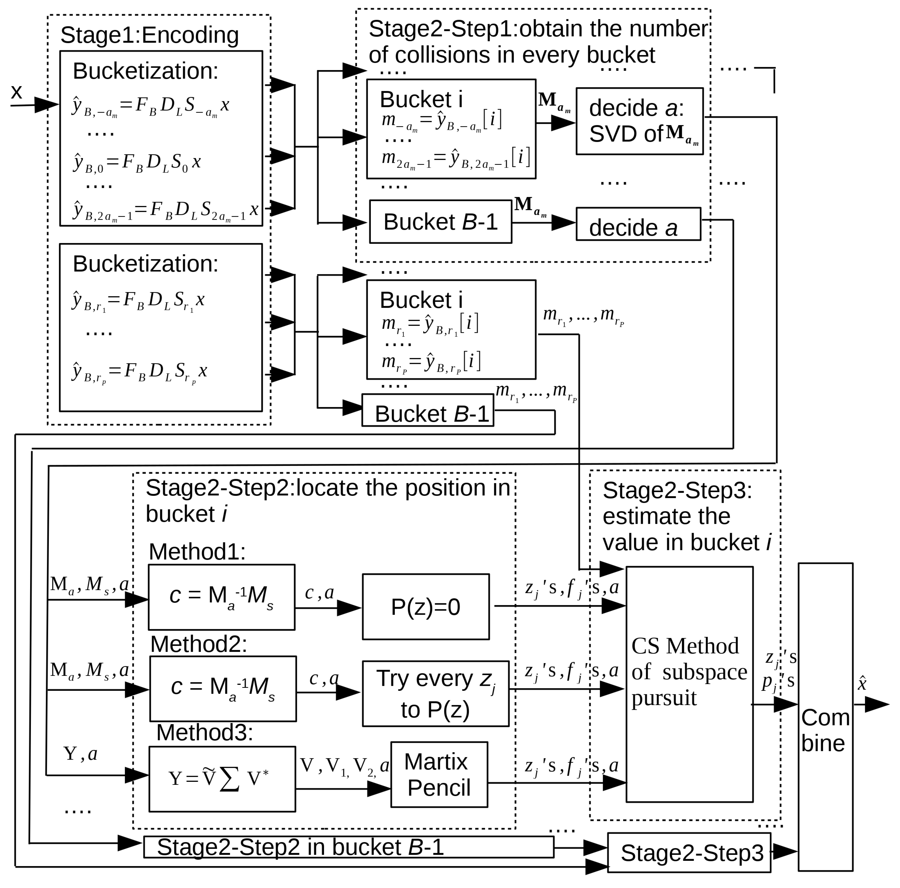
Firstly we introduce the one-shot framework, which can recover all K significant frequencies in one shot. The block diagram of the one-shot framework is shown in Figure 1. The concepts, technology, and framework involved in this section were proposed by the Taiwan university in the paper [9,10].

The first stage of sFFT is encoding by frequency bucketization. Suppose there are at most an $a_m$ number of significant frequencies aliasing in every bucket, after running 3$a_m$ times for the set $\tau =\{{\tau }_0=-a_m,{\tau }_1=-a_m+1,\dots ,{\tau }_{a_m}=0,\dots ,{\tau }_{3a_m-1}=2a_m-1\}$, calculate ${\widehat{y}}_{B,\tau }={\mathbf{F}}_B{\mathbf{D}}_L{\mathbf{S}}_{\tau }x$, representing the filtered spectrum by encoding. Suppose that in bucket i, the number of significant frequencies is denoted by a; there is a high probability that $a\le a_m$, we obtain simplified Equation (9) from Equations (7) and (8). In Equations (8) and (9), $p_j={\widehat{x}}_{f_j}$ respecting effective frequency values for $|p_0|\ge |p_1|\ge \dots \ge |p_{a-1}|\gg \mathrm{other}\mathrm{values}\mathrm{of}{p}_j$, $z_j={\omega }^{f_j}$ respecting effective frequency position for $f_j\in \left\{i,i+L,\dots ,i+(L-1)B)\right\}$, $m_k={\widehat{y}}_{B,k}\left[i\right]$ respecting filtered spectrum in bucket i for $k\in \left\{-a_m,\dots ,2a_m-1\right\}$. In most cases, $a=0$ respecting sparsity. In a small number of cases, $a=1$ respecting only one significant frequency in the bucket. Only in very few cases, $a>=2$ respecting frequencies aliasing in the bucket. It is very unlikely that $a>a_m$. In the exactly sparse case, the approximately equal sign becomes the equal sign in Equations (7)–(9), (11), (14), and (18).

The spectrum reconstruction problem in bucket i is equivalent to obtaining unknown variables including $a,z_0,\dots ,z_{a-1},p_0,\dots ,p_{a-1}$, as we have known variables including $m_{-a},\dots ,m_{2a-1}$. The aliasing problem is reformulated as a moment preserving problem (MPP). The MPP problem formulated by Bose–Chaudhuri–Hocquenghem (BCH) codes [35] can be divided into three subproblems: how to obtain a, how to obtain $z_j$’s, and how to obtain $p_j$’s in every bucket. Below, we will solve these three subproblems step by step.

$${\widehat{y}}_{B,\tau }\left[i\right]=\sum _{j=0}^{L-1}{\widehat{x}}_{jB+i}{\omega }^{\tau (jB+i)}\approx \sum _{j=0}^{a_m-1}{\widehat{x}}_{f_j}{\omega }^{\tau f_j}$$

(7)

$$m_k\approx \sum _{j=0}^{a_m-1}{p}_j{z}_j^k\approx \sum _{j=0}^{a-1}{p}_j{z}_j^k$$

(8)

$$\left[\begin{array}{cccc}{z}_0^0& z_1^0& \dots & z_{a-1}^0\\ z_0^1& z_1^1& \dots & z_{a-1}^1\\ \dots & \dots & \dots & \dots \\ z_0^{2a-1}& z_1^{2a-1}& \dots & z_{a-1}^{2a-1}\end{array}\right]\left[\begin{array}{c}{p}_0\\ p_1\\ \dots \\ p_{a-1}\end{array}\right]\approx \left[\begin{array}{c}{m}_0\\ m_1\\ \dots \\ m_{2a-1}\end{array}\right]$$

(9)

Step 1: Obtain the number of significant frequencies.

Solution: Suppose $a\le a_m$; this means $m_k$ is composed of at most an $a_m$ number of Prony component $p_j$’s. Let vector ${\widehat{z}}_j\in {\mathbb{C}}^{a_m\times 1}$ defined as ${\widehat{z}}_j={[z_j^0,z_j^1,\dots ,z_j^{a_m-1}]}^T$ and Matrix ${\mathbf{M}}_{a_m}\in {\mathbb{C}}^{a_m\times a_m}$ defined as Equation (10), then the relationship between ${\mathbf{M}}_{a_m}$, ${\widehat{z}}_j$ and ${\widehat{z}}_j^T$ satisfies Theorem 1.

$${\mathbf{M}}_{a_m}={\left[\begin{array}{cccc}{m}_0& m_1& \dots & m_{a_m-1}\\ m_1& m_2& \dots & m_{a_m}\\ \dots & \dots & \dots & \dots \\ m_{a_m-1}& m_{a_m}& \dots & m_{2a_m-1}\end{array}\right]}_{a_m\times a_m}$$

(10)

Theorem 1. 

$${\mathbf{M}}_{a_m}\approx \sum _{j=0}^{a_m-1}{p}_j{\widehat{z}}_j{\widehat{z}}_j^T$$

(11)

Proof of Theorem 1. 

$$\begin{array}{cc}\hfill & p_0{\widehat{z}}_0{z}_0^0+p_1{\widehat{z}}_1{z}_1^0+\dots +p_{a_m-1}{\widehat{z}}_{a_m-1}{z}_{a_m-1}^0\approx {[m_0,m_1,\dots ,m_{a_m-1}]}^T\hfill \\ \hfill & p_0{\widehat{z}}_0{z}_0^1+p_1{\widehat{z}}_1{z}_1^1+\dots +p_{a_m-1}{\widehat{z}}_{a_m-1}{z}_{a_m-1}^1\approx {[m_1,m_2,\dots ,m_{a_m}]}^T\hfill \\ \hfill & \dots \hfill \\ \hfill & p_0{\widehat{z}}_0{z}_0^{a_m-1}+p_1{\widehat{z}}_1{z}_1^{a_m-1}+\dots +p_{a_m-1}{\widehat{z}}_{a_m-1}{z}_{a_m-1}^{a_m-1}\approx {[m_{a_m-1},m_{a_m},\dots ,m_{2a_m}]}^T\hfill \end{array}$$

Based on the properties as mentioned above, we obtain Equation (11). □

Equation (11) is similar to the symmetric singular value decomposition (SSVD). Nevertheless, there are some differences. (1) $p_j$’s are complex but not real. (2) The columns of $[{\widehat{z}}_0,\dots ,{\widehat{z}}_{a_m-1}]$ are not mutually orthogonal normalized vectors. It is easy to perform a transformation that ${\mathbf{M}}_{a_m}\approx {\sum }_{j=0}^{a_m-1}{p}_j^{\prime }{\widehat{z^{\prime }}}_j{\widehat{z^{\prime }}}_j^T$, where $p_j^{\prime }$’s are real and the absolute value of $p_j^{\prime }$ is directly proportional to the $\left|p_j\right|$, and the columns of $[{\widehat{z^{\prime }}}_0,\dots ,{\widehat{z^{\prime }}}_{a_m-1}]$ are mutually orthogonal normalized vectors. The paper [36] proved that for the symmetric matrix, the $\Sigma$ obtained from the SVD is equal to the $\Sigma$ obtained from the SSVD. For example, the SVD of $\left[\begin{array}{cc}0& 1\\ 1& 0\end{array}\right]$ is $\left[\begin{array}{cc}0& 1\\ 1& 0\end{array}\right]=\left[\begin{array}{cc}0& 1\\ 1& 0\end{array}\right]\left[\begin{array}{cc}1& 0\\ 0& 1\end{array}\right]\left[\begin{array}{cc}1& 0\\ 0& 1\end{array}\right]$ and the SSVD of $\left[\begin{array}{cc}0& 1\\ 1& 0\end{array}\right]$ is $\left[\begin{array}{cc}0& 1\\ 1& 0\end{array}\right]=\frac{1}{\sqrt{2}}\left[\begin{array}{cc}1& -i\\ 1& i\end{array}\right]\left[\begin{array}{cc}1& 0\\ 0& 1\end{array}\right]\frac{1}{\sqrt{2}}\left[\begin{array}{cc}1& 1\\ -i& i\end{array}\right]$; the $\Sigma$ values gained via these two methods are the same. After knowing this, we can compute the SVD of ${\mathbf{M}}_{a_m}$ and obtain $a_m$ singular values, then perform the principal component analysis (PCA), ${\sigma }_1\ge {\sigma }_2\ge \dots \ge {\sigma }_{a_m}$. In these $a_m$ number of singular values ${\sigma }_j$’s, the amount of large singular values indicates the amount of efficient Prony components $p_j$’s; it also indicates how many significant frequencies are in bucket i.

Step 2: Obtain effective frequency position $f_j$’s in bucket i.

Solution: Let the orthogonal polynomial formula $P\left(z\right)$ be defined as Equation (12) and $P\left(z\right)\approx 0$. Let Matrix ${\mathbf{M}}_a\in {\mathbb{C}}^{a\times a}$ be defined as Equation (13). Let vector C be defined as $C={[c_0,c_1,\dots ,c_{a-1}]}^T$. Let vector $M_s$ be defined as $M_s=[-m_a,-m_{a+1},\dots$, $-m_{2a-1}{]}^T$. The moments’ formula satisfies Theorem 2.

$$P\left(z\right)=z^a+c_{a-1}{z}^{a-1}+\dots +c_{1}z+c_0$$

(12)

$${\mathbf{M}}_a={\left[\begin{array}{cccc}{m}_0& m_1& \dots & m_{a-1}\\ m_1& m_2& \dots & m_a\\ \dots & \dots & \dots & \dots \\ m_{a-1}& m_{a_m}& \dots & m_{2a-2}\end{array}\right]}_{a\times a}$$

(13)

Theorem 2. 

${\mathbf{M}}_{a}C\approx M_s$

$${\left[\begin{array}{cccc}{m}_0& m_1& \dots & m_{a-1}\\ m_1& m_2& \dots & m_a\\ \dots & \dots & \dots & \dots \\ m_{a-1}& m_{a_m}& \dots & m_{2a-2}\end{array}\right]}_{a\times a}{\left[\begin{array}{c}{c}_0\\ c_1\\ \dots \\ c_{a-1}\end{array}\right]}_{a\times 1}\approx {\left[\begin{array}{c}-m_a\\ -m_{a+1}\\ \dots \\ -m_{2a-1}\end{array}\right]}_{a\times 1}$$

(14)

Proof of Theorem 2. 

$$\begin{array}{cc}\hfill & c_0{m}_0\approx (p_0{z}_0^0+\dots p_{a-1}{z}_{a-1}^0)c_0\hfill \\ \hfill & \dots \hfill \\ \hfill & c_{a-1}{m}_{a-1}\approx (p_0{z}_0^{a-1}+\dots p_{a-1}{z}_{a-1}^{a-1})c_{a-1}\hfill \\ \hfill & \Rightarrow c_0{m}_0+\dots +c_{a-1}{m}_{a-1}\hfill \\ \hfill & \approx p_0(c_0{z}_0^0+\dots c_{a-1}{z}_0^{a-1})+\dots +p_{a-1}(c_0{z}_{a-1}^0+\dots c_{a-1}{z}_{a-1}^{a-1})\hfill \\ \hfill & \approx (-p_0{z}_0^a)+\dots +(-p_{a-1}{z}_{a-1}^a)\approx -m_a\hfill \end{array}$$

The first element of $M_s$ has been proven and other elements of $M_s$ can also be proven. □

For the convenience of matrix calculation, for a matrix, the superscript “T” denotes the transpose, the superscript “+” denotes the Moore–Penrose inverse or pseudoinverse, the superscript “*” denotes the adjoint matrix, and the superscript “−1” denotes the inverse. Through Theorem 2, we can obtain $C\approx \left({\mathbf{M}}_a^{-1}\right)M_s$. After gaining C, there are three ways to obtain $z_j$’s through Equation (12). The first approach is the polynomial method, the second approach is the enumeration method, and the last approach is the matrix pencil method. After knowing $z_j$’s, we can obtain the approximate positions $f_j$’s through $z_j={\omega }^{f_j}$.

(Method 1) Polynomial method: In the exactly sparse case, the a number of roots of $P\left(z\right)=0$ is the solution of $z_j$’s. For example, if $a=1$, through $P\left(z\right)=z+c_0=0$, then $z_0=-c_0$. If $a=2$, through $P\left(z\right)=z^2+c_{1}z+c_0=0$, then $z_0=(-c_1-{(c_1^2-4c_0)}^{0.5})/2,z_1=(-c_1+{(c_1^2-4c_0)}^{0.5})/2$.

(Method 2) Enumeration method: For $f_j\in \left\{i,i+L,\dots ,i+(L-1)B)\right\}$, try every possible position $z_j={\omega }^{f_j}$ in Equation (12), the first a number of the smallest $\left|P\right(z\left)\right|$ is the solution of $z_j$’s. L attempts are needed in one solution.

(Method 3) Matrix pencil method: The method was proposed in paper [37]. The matrix pencil method, like the Prony method, is a standard technique for mode frequency identification for computing the maximum likelihood signal under Gaussian noise and evenly spaced samples. For our problem, let the Toeplitz matrix $\mathbf{Y}$ be defined as Equation (15), let ${\mathbf{Y}}_{\mathbf{1}}$ be $\mathbf{Y}$ with the rightmost column removed and be defined as Equation (16), and let ${\mathbf{Y}}_{\mathbf{2}}$ be $\mathbf{Y}$ with the leftmost column removed and be defined as Equation (17). The set of generalized eigenvalues of ${\mathbf{Y}}_{\mathbf{2}}-\lambda {\mathbf{Y}}_{\mathbf{1}}$ satisfies Theorem 3.

$$\mathbf{Y}={\left[\begin{array}{cccc}{m}_0& m_{-1}& \dots & m_{-a}\\ m_1& m_0& \dots & m_{-a+1}\\ \dots & \dots & \dots & \dots \\ m_a& m_{a-1}& \dots & m_0\end{array}\right]}_{(a+1)\times (a+1)}$$

(15)

$${\mathbf{Y}}_1={\left[\begin{array}{cccc}{m}_0& m_{-1}& \dots & m_{-a+1}\\ m_1& m_0& \dots & m_{-a+2}\\ \dots & \dots & \dots & \dots \\ m_a& m_{a-1}& \dots & m_1\end{array}\right]}_{(a+1)\times \left(a\right)}$$

(16)

$${\mathbf{Y}}_2={\left[\begin{array}{cccc}{m}_{-1}& m_{-2}& \dots & m_{-a}\\ m_0& m_{-1}& \dots & m_{-a+1}\\ \dots & \dots & \dots & \dots \\ m_{a-1}& m_{a-2}& \dots & m_0\end{array}\right]}_{(a+1)\times \left(a\right)}$$

(17)

Theorem 3. 

The set of generalized eigenvalues of ${\mathbf{Y}}_{\mathbf{2}}-\lambda {\mathbf{Y}}_{\mathbf{1}}$ are the $z_j$’s we seek.

Proof of Theorem 3. 

Let the diagonal matrix $\mathbf{C}\in {\mathbb{C}}^{a\times a}$ be defined as $\mathbf{C}=\mathrm{diag}\left(p_j\right)$. Let the Vandermonde martix ${\mathbf{U}}_{a+1}\in {\mathbb{C}}^{(a+1)\times a}$ be defined as follows: ${\mathbf{U}}_{a+1}={\left[\begin{array}{cccc}1& 1& \dots & 1\\ z_0& z_1& \dots & z_{a-1}\\ \dots & \dots & \dots & \dots \\ z_0^a& z_1^a& \dots & z_{a-1}^a\end{array}\right]}_{(a+1)\times a}$. $\mathbf{Y},{\mathbf{Y}}_{\mathbf{1}},{\mathbf{Y}}_{\mathbf{2}}$ has a Vandermonde decomposition, we can obtain $\mathbf{Y}=\frac{1}{a+1}{\mathbf{U}}_{a+1}\mathbf{C}{\mathbf{U}}_{a+1}^{*}$, ${\mathbf{Y}}_1=\frac{1}{a+1}{\mathbf{U}}_{a+1}\mathbf{C}{\mathbf{U}}_a^{*}$, ${\mathbf{Y}}_2=\frac{1}{a+1}{\mathbf{U}}_{a+1}\mathbf{C}\left(\mathrm{diag}{\left(z_j\right)}^{*}\right){\mathbf{U}}_a^{*}$. For example, if a = 1, $\mathbf{Y}=\left[\begin{array}{cc}{m}_0& m_{-1}\\ m_1& m_0\end{array}\right]=\left[\begin{array}{cc}{p}_0& p_0{z}_0^{-1}\\ p_0{z}_0^1& p_0\end{array}\right]=\left[\begin{array}{c}1\\ z_0\end{array}\right]p_0\left[\begin{array}{cc}1& z_0^{-1}\end{array}\right]$, and if a = 2, $\mathbf{Y}=\left[\begin{array}{ccc}{m}_0& m_{-1}& m_{-2}\\ m_1& m_0& m_{-1}\\ m_2& m_1& m_0\end{array}\right]=\left[\begin{array}{ccc}{p}_0+p_1& p_0{z}_0^{-1}+p_1{z}_1^{-1}& p_0{z}_0^{-2}+p_1{z}_1^{-2}\\ p_0{z}_0^1+p_1{z}_1^1& p_0+p_1& p_0{z}_0^{-1}+p_1{z}_1^{-1}\\ p_0{z}_0^2+p_1{z}_1^2& p_0{z}_0^1+p_1{z}_1^1& p_0+p_1\end{array}\right]=\left[\begin{array}{cc}1& 1\\ z_0& z_1\\ z_0^2& z_1^2\end{array}\right]\left[\begin{array}{cc}{p}_0& \\ & p_1\end{array}\right]\left[\begin{array}{ccc}1& z_0^{-1}& z_0^{-2}\\ 1& z_1^{-1}& z_1^{-2}\end{array}\right]$, ${\mathbf{Y}}_1=\left[\begin{array}{cc}{m}_0& m_{-1}\\ m_1& m_0\\ m_2& m_1\end{array}\right]=\left[\begin{array}{cc}1& 1\\ z_0& z_1\\ z_0^2& z_1^2\end{array}\right]\left[\begin{array}{cc}{p}_0& \\ & p_1\end{array}\right]\left[\begin{array}{cc}1& z_0^{-1}\\ 1& z_1^{-1}\end{array}\right]$, ${\mathbf{Y}}_2=\left[\begin{array}{cc}{m}_{-1}& m_{-2}\\ m_0& m_{-1}\\ m_1& m_0\end{array}\right]=\left[\begin{array}{cc}1& 1\\ z_0& z_1\\ z_0^2& z_1^2\end{array}\right]\left[\begin{array}{cc}{p}_0& \\ & p_1\end{array}\right]\left[\begin{array}{cc}{z}_0^{-1}& \\ & z_1^{-1}\end{array}\right]\left[\begin{array}{cc}1& z_0^{-1}\\ 1& z_1^{-1}\end{array}\right]$. Using the Vandermonde decomposition, and we can obtain ${\mathbf{Y}}_2-\lambda {\mathbf{Y}}_1=\frac{1}{a+1}{\mathbf{U}}_{a+1}\mathbf{C}(\mathrm{diag}{\left(z_j\right)}^{*}-\lambda \mathbf{I}){\mathbf{U}}_a^{*}$, so the Theorem 3 can be proven. □

If the rank $\left(\mathbf{Y}\right)=a$, the set of generalized eigenvalues of ${\mathbf{Y}}_{\mathbf{2}}-\lambda {\mathbf{Y}}_{\mathbf{1}}$ is equal to the set of nonzero${}^2$ ordinary eigenvalues of $\left({\mathbf{Y}}_{\mathbf{1}}^{+}\right){\mathbf{Y}}_{\mathbf{2}}$. It is most likely that for the rank $\left(\mathbf{Y}\right)<a$, it is necessary to compute the SVD of the $\mathbf{Y}$, $\mathbf{Y}=\tilde{\mathbf{V}}\Sigma {\mathbf{V}}^{*}$, and then we can use the matrix pencil method to deal with the matrix $\mathbf{V}$ afterword. For details, please refer to paper [7,37].

Step 3: Obtain effective frequency values $p_j$’s in bucket i.

Solution: In order to use the CS method, we need several random samplings. Thus, for a P number of random numbers $r_1,\dots ,r_P$, we calculate ${\widehat{y}}_{B,\tau }={\mathbf{F}}_B{\mathbf{D}}_L{\mathbf{S}}_{\tau }x$ for the set $\tau =\left\{{\tau }_0=r_1,{\tau }_1=r_2,\dots ,{\tau }_{P-1}=r_P\right\}$ in a P times’ round. Suppose that in bucket i, the number of significant frequencies a and approximate effective frequency position $z_j$’s have been known by step 1 and step 2; we can obtain Equation (18). (There may be errors for $z_j$’s obtained by step 2 because of the interference of another $L-a$ number of Prony components).

$${\left[\begin{array}{c}{m}_1\\ \dots \\ m_P\end{array}\right]}_{P\times 1}={\left[\begin{array}{ccc}{z}_0^{r_1}& \dots & z_{L-1}^{r_1}\\ \dots & \dots & \dots \\ z_0^{r_P}& \dots & z_{L-1}^{r_P}\end{array}\right]}_{P\times L}{\left[\begin{array}{c}{p}_0\\ \dots \\ p_{L-1}\end{array}\right]}_{L\times 1}\approx {\left[\begin{array}{ccc}{z}_0^{r_1}& \dots & z_{a-1}^{r_1}\\ \dots & \dots & \dots \\ z_0^{r_P}& \dots & z_{a-1}^{r_P}\end{array}\right]}_{P\times a}{\left[\begin{array}{c}{p}_0\\ \dots \\ p_{a-1}\end{array}\right]}_{a\times 1}$$

(18)

Equation (18) is very likely similar to the CS formula. The model of CS is formulated as $y\approx \Phi S$, where S is a sparse signal, $\Phi$ is a sensing matrix, and y is the measurements. In Equation (18), y is a vector of $P\times 1$ by P measurements, $\Phi$ is a matrix of $P\times L$, and S is a vector of $L\times 1$ that is a-sparse. It should be noted that $\Phi$ must satisfy either the restricted isometry property (RIP) or mutual incoherence property (MIP) for a successful recovery with high probability. It has been known that the Gaussian random matrix and partial Fourier matrix are good candidates to be $\Phi$, so the $\Phi$ of Equation (18) meets the criteria. Furthermore, the number of measurements P one collects should be more than $a{\log }_{10}L$, so that these measurements will be sufficient to recover signal x.

In order to obtain $p_j$’s using the CS solver, we use the subspace pursuit method. The process is as follows: (1) Through the positions $f_j$’s gained by step 2, obtain the possible value of $z_j$’s as follows: $z_j^{\prime }={\omega }^{f_j}$, $z_j^{\prime \prime }={\omega }^{f_j+B}$, $z_j^{\prime \prime \prime }={\omega }^{f_j-B}$, then obtain 3a vectors as follows: ${\{{z_0^{\prime }}^{r_1},\dots ,{z_0^{\prime }}^{r_P}\}}^T,{\{{z_0^{\prime \prime }}^{r_1},\dots ,{z_0^{\prime \prime }}^{r_P}\}}^T$, ${\{{z_0^{\prime \prime \prime }}^{r_1},\dots ,{z_0^{\prime \prime \prime }}^{r_P}\}}^T,\dots {\{{z_{a-1}^{\prime \prime \prime }}^{r_1},\dots ,{z_{a-1}^{\prime \prime \prime }}^{r_P}\}}^T$. An (over-complete) dictionary can be characterized by a matrix $\mathbf{D}$, and it contains the $3a$ vectors listed above. (One wishes one-third vectors of them form a basis). Each (column) vector in a dictionary is called an atom. (2) From $3a$ atoms of the dictionary matrix $\mathbf{D}$, find a number of atoms that best match the measurements’ residual error. Select these a number of atoms to construct a new sensing matrix $\widehat{\Phi }$. (3) Obtain $\widehat{S}$ by the support of $\widehat{S}=\mathrm{argmin}{∥y-\widehat{\Phi }\widehat{S}∥}_2$ through the least square method (LSM). (4) If the residual error ${∥y-\widehat{\Phi }\widehat{S}∥}_2$ meets the requirement, or the number of iterations reaches the assumption, or the residual error becomes larger, the iteration will be quit; otherwise continue to step 2. After computing, we obtain the final sensing matrix $\widehat{\Phi }$ of size $P\times a$ and sparse signal $\widehat{S}$ of size a just in the right part of Equation (18). Thus we obtain effective frequency positions $z_j$’s and effective frequency values $p_j$’s in bucket i.

3.2. Peeling Framework Based on the Bipartite Graph

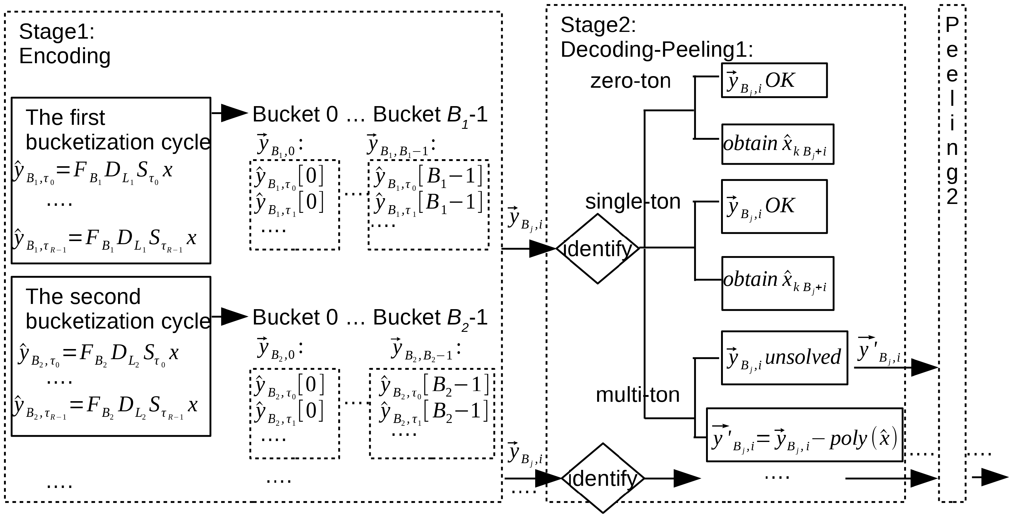
Secondly, we introduce the peeling framework, which can recover all K significant frequencies layer by layer. The block diagram of the peeling framework is shown in Figure 2. The concepts, technology, and framework involved in this section were proposed by Berkeley university in the paper [11,12,13,14].

In the peeling framework, we require the size N of signal x to be a product of a few (typically three or more) co-prime numbers $p_i$’s. For example $N=p_1{p}_2{p}_3$, where $p_1,p_2,p_3$ are co-prime numbers. With this precondition, we determine $L_i$’s and $B_i$’s gained from $p_i$’s in each bucketization cycle. In every cycle, we use the same set $\tau =\left\{{\tau }_0=r_1,{\tau }_1=r_2,\dots ,{\tau }_{R-1}=r_R\right\}$ inspired by different spectrum reconstruction methods introduced later to calculate ${\widehat{y}}_{B,\tau }={\mathbf{F}}_B{\mathbf{D}}_L{\mathbf{S}}_{\tau }x$ in R times’ rounds (this also means there are R delay chains for one bucket). Suppose there are d cycles, after d cycles, stage 1 encoding by bucketization is completed. In order to solve the aliasing problems, the filtered spectrum in bucket i of the no. j’ cycle is denoted by vector ${\overrightarrow{y}}_{B_j,i}\in {\mathbb{C}}^{R\times 1}$ as follows:

$${\overrightarrow{y}}_{B_j,i}=\left[\begin{array}{c}{\widehat{y}}_{B_j,{\tau }_0}\left[i\right]\\ \dots \\ {\widehat{y}}_{B_j,{\tau }_{R-1}}\left[i\right]\end{array}\right]=\left[\begin{array}{c}\sum _{k=0}^{L_j-1}{\widehat{x}}_{(k{B}_j+i)}{\omega }^{{\tau }_0(k{B}_j+i)}\\ \dots \\ \sum _{k=0}^{L_j-1}{\widehat{x}}_{(k{B}_j+i)}{\omega }^{{\tau }_{R-1}(k{B}_j+i)}\end{array}\right]$$

(19)

We use a simple example to illustrate the process of encoding by bucketization. Consider a signal x of size (N = 20) that has only five (K = 5) significant coefficients, ${\widehat{x}}_1,{\widehat{x}}_3,{\widehat{x}}_5,{\widehat{x}}_{10},{\widehat{x}}_{13}>>0$, while the rest of the coefficients are approximately equal to zero. With this precondition, there are two bucketization cycles. In the first cycle, for $B_1=4$ and $L_1=5$, we obtain four vectors, $\{{\overrightarrow{y}}_{4,0},{\overrightarrow{y}}_{4,1},{\overrightarrow{y}}_{4,2},{\overrightarrow{y}}_{4,3}\}$, respecting the filtered spectrum in four buckets for the set $\tau$ in R rounds. In the second cycle, for $B_2=5$ and $L_2=4$, we obtain five vectors, $\{{\overrightarrow{y}}_{5,0},{\overrightarrow{y}}_{5,1},{\overrightarrow{y}}_{5,2},{\overrightarrow{y}}_{5,3},{\overrightarrow{y}}_{5,4}\}$. 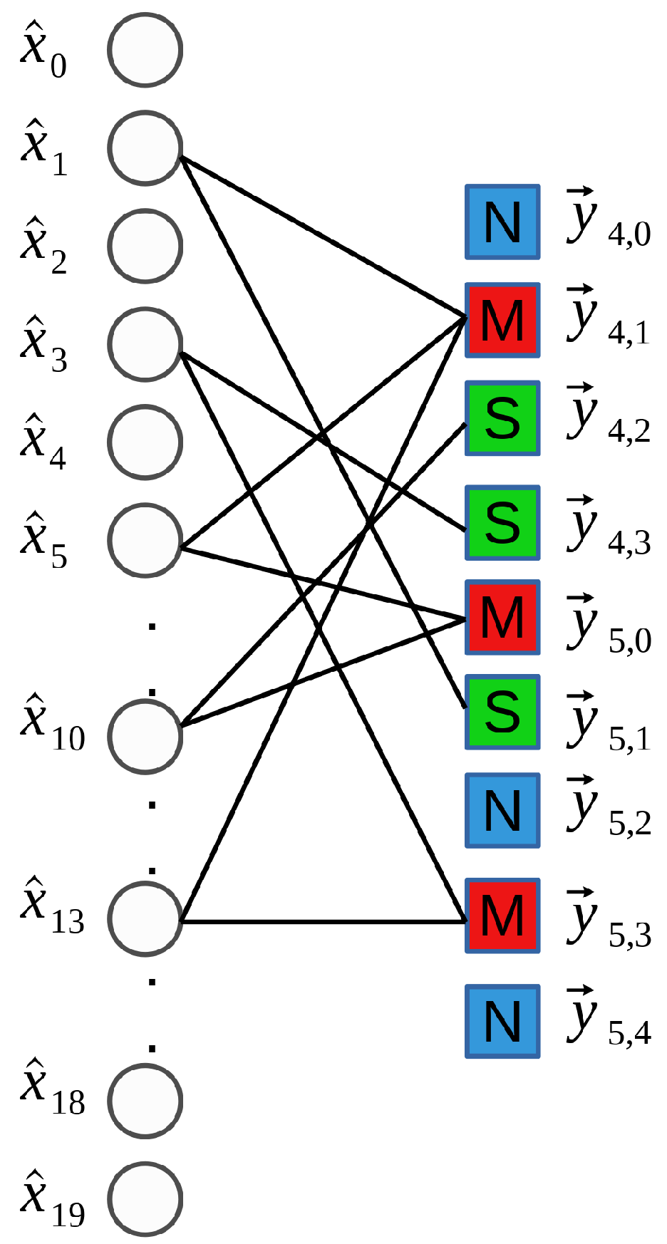After the bucketization, we can construct a bipartite graph shown in Figure 3 through Equation (19). In Figure 3, there are $N=20$ variable nodes on the left (referring to the 20 coefficients of $\widehat{x}$) and $N_b=B_1+B_2=4+5=9$ parity check nodes on the right (referring to nine buckets in two cycles). The values of the parity check nodes on the right are approximately equal to the complex sum of the values of variable nodes (its left neighbors) through Equation (19). In these check nodes, some have no significant variable node with no left neighbor, which is called a “zero-ton” bucket (three blue-colored check nodes). Some have exactly one significant variable node, as one left neighbor, which is called a “single-ton” bucket (three green-colored check nodes). Others have more than one significant variable nodes, as more than one left neighbors, which is called a “multi-ton” bucket (three red-colored check nodes).

After bucketization, the subsequent problem is how to recover the spectrum from all buckets gained from several cycles. Through the identification of vector ${\overrightarrow{y}}_{B_j,i}$, we can determine the characteristics of bucket $B_j\left[i\right]$. If the bucket is a “zero-ton” bucket, then ${\widehat{x}}_{(k{B}_j+i)}=0\mathrm{for}k\in [0,L_j-1]$, so the problem of frequency recovery in this bucket can be solved. If the bucket is a “single-ton” bucket, suppose the one effective frequency position $f_0$ and the one effective frequency value ${\widehat{x}}_{f_0}$ can be obtained by the afterward methods, then ${\widehat{x}}_{(k{B}_j+i)}=\left\{\begin{array}{c}0\mathrm{for}(k\in [0,L_j-1])\cap (k{B}_j+i\ne f_0)\\ {\widehat{x}}_{f_0}\mathrm{for}k{B}_j+i=f_0\end{array}\right.$, and thus the frequency recovery in this bucket can be solved. If the bucket is a “multi-ton” bucket, it is necessary to separate the “multi-ton” bucket into the “single-ton” bucket to realize the decoding of the “multi-ton” bucket. For example, after the first peeling, in the bucket i of the no. j cycle, suppose ${\widehat{x}}_{f_0},\dots {\widehat{x}}_{f_{n_1-1}}$ have been obtained via another “single-ton” bucket, then the vector ${\overrightarrow{y}}_{B_j,i}$ respecting the original bucket changes to ${\overrightarrow{y}}_{B_j,i}^{\prime }$, where ${\overrightarrow{y}}_{B_j,i}^{\prime }={\overrightarrow{y}}_{B_j,i}-\mathrm{poly}\left({\widehat{x}}_{f_0}\right)-\dots -\mathrm{poly}\left({\widehat{x}}_{f_{n_1-1}}\right)$ respecting the remaining frequencies in the bucket. Through the identification of vector ${\overrightarrow{y}}_{B_j,i}^{\prime }$, we can analyze the remaining elements in this bucket; if it is a “zero-ton” bucket or a “single-ton” bucket, we can stop peeling and obtain all frequencies in this bucket. If not, continue the second peeling, and suppose ${\widehat{x}}_{f_{n_1}},\dots {\widehat{x}}_{f_{n_2-1}}$ can be obtained by another “single-ton” bucket through new peeling. We can identify ${\overrightarrow{y}}_{B_j,i}^{\prime \prime }$ to continue to analyze the bucket, where ${\overrightarrow{y}}_{B_j,i}^{\prime \prime }={\overrightarrow{y}}_{B_j,i}^{\prime }-\mathrm{poly}\left({\widehat{x}}_{f_{n_1}}\right)-\dots -\mathrm{poly}\left({\widehat{x}}_{f_{n_2-1}}\right)$. After q times’ peeling, the problem of frequency recovery in the “multi-ton” bucket can be solved as follows:

$${\widehat{x}}_{(k{B}_j+i)}=\left\{\begin{array}{c}0\mathrm{for}(k\in [0,L_j-1])\cap (k{B}_j+i\ne f_0)\cap \dots \cap (k{B}_j+i\ne f_{n_q-1})\\ {\widehat{x}}_{f_0}\mathrm{for}k{B}_j+i=f_0\\ \dots \\ {\widehat{x}}_{f_{n_q-1}}\mathrm{for}k{B}_j+i=f_{n_q-1}\end{array}\right.$$

(20)

If the frequency recovery in all buckets can be solved, we can finish the spectrum reconstruction. The peeling-decoder successfully recovers all of the frequencies with high probability under the three following assumptions: (1) “Zero-ton”, “single-ton” and “multi-ton” buckets can be identified correctly. (2) If the bucket is a “single-ton” bucket, the decoder can locate the effective frequency position $f_0$ and estimate the effective frequency value ${\widehat{x}}_{f_0}$ correctly. (3) It is sufficient to cope with “multi-ton” buckets via the peeling platform.

Subproblem 1: How to identify vector ${\overrightarrow{y}}_{B_j,i}$ to distinguish bucket $B_j\left[i\right]$?

Solution: In the exactly sparse case, if ${∥{\overrightarrow{y}}_{B_j,i}∥}_2=0$, the bucket is a “zero-ton” bucket. If the bucket is not a “zero-ton” bucket, make the second judgment. The way to make the second judgment about whether the bucket is a ”single-ton” bucket or not is to judge ${∥{\overrightarrow{y}}_{B_j,i}-\mathrm{poly}\left({\widehat{x}}_{f_0}\right)∥}_2=0\mathrm{or}\ne 0$, where ${\widehat{x}}_{f_0}$ is gained from the solution of subproblem 2. If the bucket $B_j\left[i\right]$ is not a “zero-ton” bucket nor a “single-ton” bucket, it is a “multi-ton” bucket. In the general sparse case, the two equations are translated to ${∥{\overrightarrow{y}}_{B_j,i}∥}_2\le T_0$ and ${∥{\overrightarrow{y}}_{B_j,i}-\mathrm{poly}\left({\widehat{x}}_{f_0}\right)∥}_2\le T_1$, where $T_0$ and $T_1$ are the identification thresholds. It costs $O\left(R\right)$ runtime to identify vector ${\overrightarrow{y}}_{B_j,i}$ by knowing ${\widehat{x}}_{f_0}$ in advance. After d cycles, $O\left(R(B_1+\dots +B_d)\right)$ runtime is needed for the identification in the first peeling.

Subproblem 2: Suppose the target is a “single-ton” bucket, how to recover the one frequency in this bucket?

Solution: In the exactly sparse case, we use $R=3$ and the set $\tau =\left\{{\tau }_0=0,{\tau }_1=1,{\tau }_2=2\right\}$ to calculate ${\widehat{y}}_{B,\tau }={\mathbf{F}}_B{\mathbf{D}}_L{\mathbf{S}}_{\tau }x$ in three rounds. Suppose the bucket $B_j\left[i\right]$ is a ”single-ton” bucket, then three elements of the vector ${\overrightarrow{y}}_{B_j,i}$ are ${\widehat{y}}_{B_j,0}\left[i\right]={\widehat{x}}_{f_0}{\omega }^{0·f_0}$, ${\widehat{y}}_{B_j,1}\left[i\right]={\widehat{x}}_{f_0}{\omega }^{1·f_0}$ and ${\widehat{y}}_{B_j,2}\left[i\right]={\widehat{x}}_{f_0}{\omega }^{2·f_0}$. Thus, only if $\frac{{\widehat{y}}_{B_j,0}\left[i\right]}{{\widehat{y}}_{B_j,1}\left[i\right]}=\frac{{\widehat{y}}_{B_j,1}\left[i\right]}{{\widehat{y}}_{B_j,2}\left[i\right]}$, it is a ”single-ton” bucket. If it is a ”single-ton” bucket, the position $f_0$ can be obtained by $f_0=\angle \frac{{\widehat{y}}_{B_j,1}\left[i\right]}{{\widehat{y}}_{B_j,0}\left[i\right]}·\left(\frac{-N}{2\pi }\right)$, and the value ${\widehat{x}}_{f_0}$ can be obtained by ${\widehat{x}}_{f_0}={\widehat{y}}_{B_j,0}\left[i\right]$. In all, it costs three samples and four runtimes to recover the one significant frequency in one bucket.

In the general sparse case, the frequency recovery method is the optimal whitening filter coefficient of the minimum mean squared error (MMSE) estimator and sinusoidal structured bin-measurement matrix for the speedy recovery. At first, the set of the one candidate $f_0$ is $f_0\in \left\{i,i+L,\dots ,i+(L-1)B)\right\}$, and there are L possible choices. In the first iteration of the binary search, we choose a random number $r_0$, then calculate ${\widehat{y}}_{B_j,r_0},{\widehat{y}}_{B_j,r_0+1},\dots ,{\widehat{y}}_{B_j,r_0+m-1}$ in m rounds. In fact, we obtain ${\widehat{y}}_{B_j,r_0}\left[i\right]\approx {\widehat{x}}_{f_0}{\omega }^{\left(r_0\right)·f_0},{\widehat{y}}_{B_j,r_0+1}\left[i\right]\approx {\widehat{x}}_{f_0}{\omega }^{(r_0+1)·f_0},\dots ,{\widehat{y}}_{B_j,r_0+m-1}\left[i\right]\approx {\widehat{x}}_{f_0}{\omega }^{(r_0+m-1)·f_0}$. ${\Delta }_t$ respecting the phase difference is defined as ${\Delta }_t=\angle {\widehat{y}}_{B_j,r_0+t+1}\left[i\right]-\angle {\widehat{y}}_{B_j,r_0+t}\left[i\right]=\angle {\omega }^{f_0}+U_{t+1}-U_t$, where $U_t$ relates to the real error in no. t’ round. In paper [38], we can see the maximum likelihood estimate (MLE) $\angle {\widehat{\omega }}^{f_0}$ of $\angle {\omega }^{f_0}$ is calculated by Equation (21), where $w_t$ is defined as Equation (22). After obtaining $\angle {\widehat{\omega }}^{f_0}$, make a judgment of binary search; if $\angle {\widehat{\omega }}^{f_0}\in [0,\pi ]$, there is a new restriction that $f_0\in [0,N/2-1]$, otherwise the restriction is $f_0\in [N/2,N-1]$ the complement set of set $[0,N/2-1]$. The next iteration is very similar; we choose a random number $r_1$, then calculate ${\widehat{y}}_{B_j,r_1}\left[i\right],{\widehat{y}}_{B_j,r_1+2}\left[i\right],\dots ,{\widehat{y}}_{B_j,r_1+2(m-1)}\left[i\right]$ in bucket i. After obtaining $\angle {\widehat{\omega }}^{2f_0}$ through Equations (21) and (22), we make a judgment of binary-search; if $\angle {\widehat{\omega }}^{2f_0}\in [0,\pi ]$, there is a new restriction that $f_0\in [0,N/4-1]\cup [N/2,3N/4-1]$, otherwise the restriction is the complement set of the previous set. After C iterations, in the advantage of restrictions, we can locate the only position $f_0$ from the original set $\left\{i,i+B,\dots ,i+(L-1)B)\right\}$. From the paper [13], if the number of iterations $C=O\left(\log N\right)$ and the number of rounds per iteration $m=O\left({\log }^{1/3}N\right)$, the singleton-estimator algorithm can correctly identify the unknown frequency $f_0$ with a high probability. If the signal-to-noise ratio (SNR) is low, the m and C must be increased. After knowing $f_0$, we can obtain ${\widehat{x}}_{f_0}$ by applying the LSM. In all, to recover the one approximately significant frequency in one bucket, it needs $Cm=O\left({\log }^{4/3}N\right)$ samples and $3Cm=O\left({\log }^{4/3}N\right)$ runtime. The runtime includes $Cm$ runtime to calculate all ${\Delta }_t$’s and $2Cm$ runtime to calculate all $\angle {\widehat{\omega }}^{2^j{f}_0}$’s. ${\widehat{x}}_{f_0}$ can be used to judge whether the bucket is a “single-ton” bucket or not through the discriminant ${\overrightarrow{y}}_{B_j,i}-\mathrm{poly}\left({\widehat{x}}_{f_0}\right)\le T_1$.

$$\angle {\widehat{\omega }}^{f_0}=\sum _{t=0}^{m-2}{w}_t{\Delta }_t$$

(21)

$$w_t=\frac{3m}{2(m^2-1)}(1-4{\left(\frac{2t-m+2}{2m}\right)}^2)$$

(22)

Subproblem 3: How to solve the “multi-ton” buckets by the peeling platform?

Solution with method 1: The genie-assisted peeling decoder by the bipartite graph is useful. As shown in Figure 3, the bipartite graph represents the characteristics of the bucketization. The variable nodes on the left represent the characteristics of the frequencies. The parity check nodes on the right represent the characteristics of the buckets. 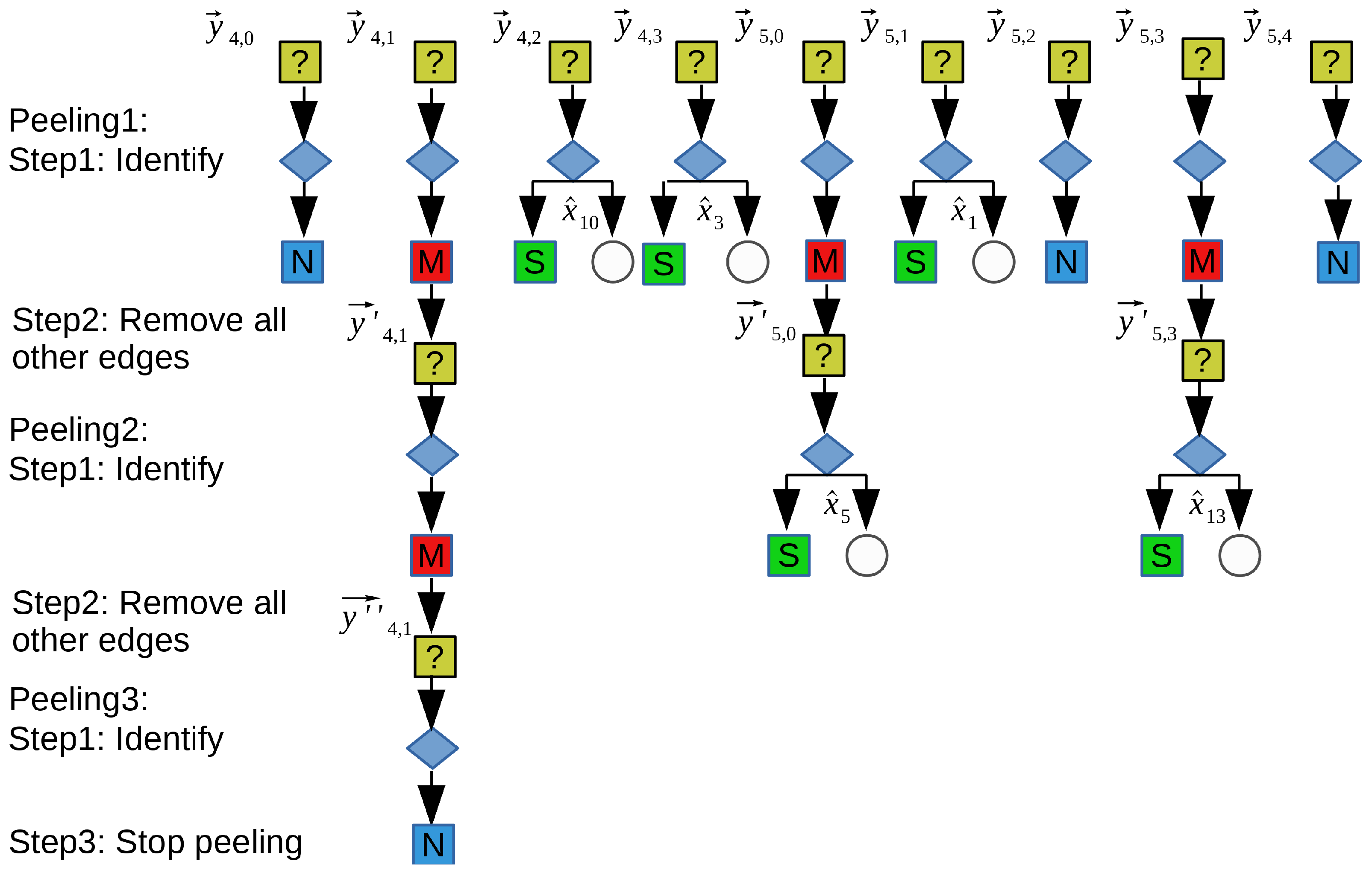Every efficient variable node connects d different parity check nodes as its neighbors in d cycles; it respects the d edges connected to each efficient variable node. The example of the process of the genie-assisted peeling decoder is shown in Figure 4, and the steps are as follows:

Step 1: We can identify all the indistinguishable buckets. If the bucket is a “zero-ton” bucket, the frequency recovery in this bucket is finished. If the bucket is a “single-ton” bucket, we can obtain the frequency in the bucket through the solution of subproblem 2. In the graph, these operations represent to select and remove all right nodes with degree 0 or degree 1, and moreover, to remove the edges connected to these right nodes and corresponding left nodes.

Step 2: We should remove the contributions of these frequencies gained by step 1 in other buckets. For example, the first peeling in bucket i means we calculate a new vector ${\overrightarrow{y^{\prime }}}_{B_j,i}$ just as ${\overrightarrow{y^{\prime }}}_{B_j,i}={\overrightarrow{y}}_{B_j,i}-\mathrm{poly}\left({\widehat{x}}_{f_0}\right)-\dots -\mathrm{poly}\left({\widehat{x}}_{f_{n_1-1}}\right)$, where ${\widehat{x}}_{f_0},\dots {\widehat{x}}_{f_{n_1-1}}$ have been gained by step 1. In the graph, these operations represent removing all the other edges connected to the left nodes removed in step 1. When the edges are removed, their contributions are subtracted from their right nodes. In the new graph, the degree of some right nodes decreases as well.

Step 3: If all buckets have been identified, we successfully reconstruct the spectrum $\widehat{x}$. Otherwise, we turn to step 1 and step 2 to continue identifying and peeling operations. In the graph, it means that if all right nodes are removed, the decoding is finished. Otherwise, turn to step 1 and step 2.

Solution with method 2: The sparse-graph decoder by the packet erasure channel method is more efficient. From Figure 4, we see all processes need 13 (9 + 3 + 1) identifications in three peelings, so it is not very efficient. As we can see, spectrum recovery can transform into a problem of decoding over sparse bipartite graphs using the peeling platform. The problem of decoding over sparse bipartite graphs has been well studied in the coding theory literature. From the coding theory literature, we know that several sparse-graph code constructions are of low-complexity and capacity-achieving by using the erasure channels method. Thus we use the erasure channels method to improve efficiency.

We construct a bipartite graph with K variable nodes on the left and $N_b$ check nodes on the right. Each efficient left node ${\widehat{x}}_f$ connects exactly d right nodes ${\overrightarrow{y}}_{B_j,i}$’s in d cycles and the set of $N_b$ check nodes are assigned to d subsets with the no. i’s subset having $B_i$ check nodes. The example of the “balls-and-bins” model defined above is shown in Figure 2. In Figure 3, there are $K(K=5)$ variable nodes on the left and $N_b(N_b=9)$ check nodes on the right and each left node ${\widehat{x}}_f$ connects exactly $d(d=2)$ right nodes; the set of check nodes is assigned to two subsets ($\{{\overrightarrow{y}}_{4,0},{\overrightarrow{y}}_{4,1},{\overrightarrow{y}}_{4,2},{\overrightarrow{y}}_{4,3}\},\{{\overrightarrow{y}}_{5,0},{\overrightarrow{y}}_{5,1},{\overrightarrow{y}}_{5,2},{\overrightarrow{y}}_{5,3},{\overrightarrow{y}}_{5,4}\}$). If one left node is selected, a d number of its neighboring right nodes will be determined. If one right node is selected, an L number of its neighboring left nodes will be determined as well. These two corresponding nodes are connected through an edge (in the graph, if the variable nodes on the left are efficient nodes, the edge is a solid line. Otherwise, the edge is a dotted line or is omitted). A directed edge $\overrightarrow{e}$ in the graph is represented as an ordered pair of nodes such as $\overrightarrow{e}=\{V,C\}$ or $\overrightarrow{e}=\{C,V\}$, where V is a variable node and C is a check node. A path in the graph is a directed sequence of directed edges such as $\left\{\overrightarrow{e_1},\dots ,\overrightarrow{e_l}\right\}$, where the end node of the previous edge of the path is the start node of the next edge of the path. Depth l is defined as the length of the path, which also indicates the number of directed edges in the path. The induced subgraph $N_V^l$ is the directed neighborhood of depth l of left node V. It contains all of the edges and nodes on paths $\overrightarrow{e_1},\dots ,\overrightarrow{e_l}$ starting at node V. It is a tree-like graph that can be seen in Figure 5. In Figure 5, it can be seen that subgraph $N_V^l$ starting at ${\widehat{x}}_2$ with depth l is equal to two, three, four, five, and six, and subgraph $N_V^l$ starting at ${\widehat{x}}_7$ with depth l is equal to six. Under these definitions, we obtain the steps of thepacket erasure channel method as follows: Step 1: Take $O\left(K\right)$ random left nodes as starting points, and draw $O\left(K\right)$ trees $N_V^1$ from these starting points. As shown in Figure 5, we choose two left nodes ${\widehat{x}}_2$ and ${\widehat{x}}_7$ as starting points. The endpoints of $N_V^1$ are check nodes; we then identify the characteristics of these check nodes. If the check node is a “zero-ton” bucket, such as ${\overrightarrow{y}}_{5,2}$, this path stops extending. If the check node is a “multi-ton” bucket, continue waiting until its left neighboring node is identified by other paths. If the check node is a “single-ton” bucket, such as ${\overrightarrow{y}}_{4,2}$ and ${\overrightarrow{y}}_{4,3}$, continue to connect its only efficient left neighboring node. Then obtain the tree $N_V^2$ through expending these left nodes. Their $(d-1)$ number of new right neighboring nodes will be determined through these left nodes; then, obtain the tree $N_V^3$ by expending these right nodes.

…

Step p: For each start-point V, we have obtained tree $N_V^{2p-1}$ from the last step. The endpoints of $N_V^{2p-1}$ are check nodes. We should remove the contributions of some frequencies gained by the previous paths at first, then identify the characteristics of these modified check nodes. For example, before identifying ${\overrightarrow{y}}_{5,0}$, the endpoint of $N_{{\widehat{x}}_2}^3$, we should remove the contributions of ${\widehat{x}}_{10}$. Furthermore, before identifying ${\overrightarrow{y}}_{4,1}$, the endpoint of $N_{{\widehat{x}}_2}^5$, we should remove the contributions of ${\widehat{x}}_{13}$ and ${\widehat{x}}_5$. If the modified check node is a “zero-ton” bucket, this path stops extending. If the modified check node is a “multi-ton” bucket, continue waiting until its left neighboring node is identified by other paths. If the modified check node is a “single-ton” bucket, continue to connect its only efficient left neighboring node. Then obtain the tree $N_V^{2p}$ through expending these left nodes. Their $(d-1)$ number of new right neighboring nodes will be determined through these left nodes; then obtain the tree $N_V^{2p+1}$ by expending these right nodes.

If the number of left nodes identified is equal to K, it means the spectrum recovery has been successful. The example is shown in Figure 5. In Figure 5, from the beginning of starting points ${\widehat{x}}_2$ and ${\widehat{x}}_7$, we can obtain two trees, $N_{{\widehat{x}}_2}^6$ and $N_{{\widehat{x}}_7}^6$ (depth = 6), through three expanding by three steps. From the graph, we can obtain all five variable nodes. All processes need six (4 + 4 − 2) identifications, which is far less than the thirteen identifications of method 1.

3.3. Iterative Framework Based on the Binary Tree Search Method

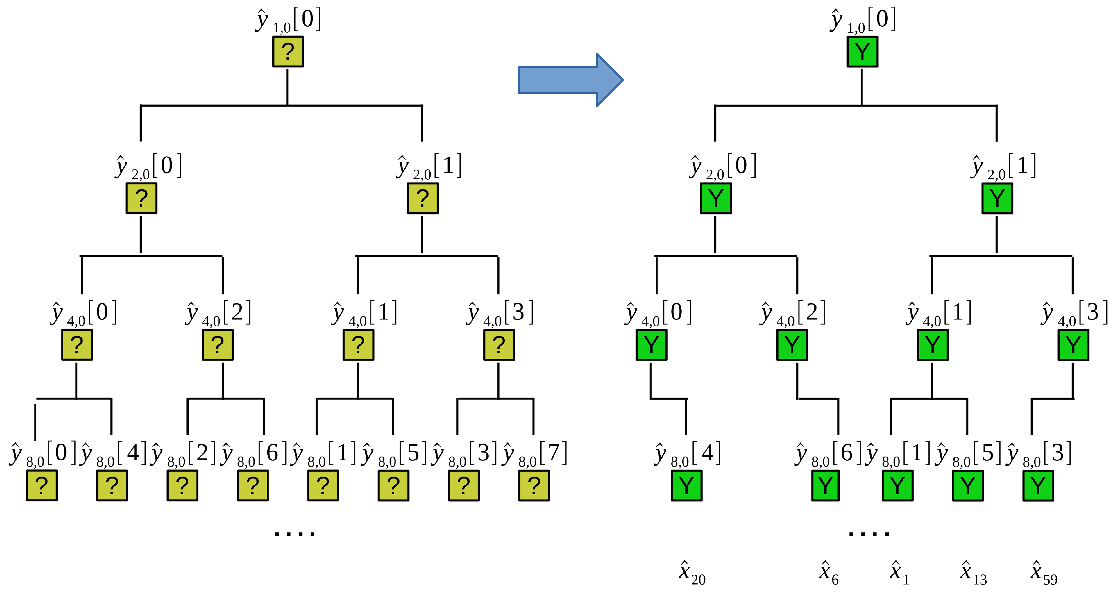
Thirdly, we introduce the iterative framework based on the binary tree search method. The example is shown in Figure 6. The concepts, technology, and framework involved in this section were proposed by Georg-August university in the paper [15].

Consider a signal $\widehat{x}$ sized $N=64$ that has only five ($K=5$) significant coefficients ${\widehat{x}}_1,{\widehat{x}}_6,{\widehat{x}}_{13},{\widehat{x}}_{20},{\widehat{x}}_{59}>>0$, while the rest of the coefficients are approximately equal to zero. The node of the first layer of the binary tree is ${\widehat{y}}_{1,0}\left[0\right]={\sum }_{j=0}^{N-1}{\widehat{x}}_j$, with N aliasing frequencies. The nodes of the second layer of the binary tree are ${\widehat{y}}_{2,0}\left[0\right]={\sum }_{j=0}^{N/2-1}{\widehat{x}}_{2j}$ and ${\widehat{y}}_{2,0}\left[1\right]={\sum }_{j=0}^{N/2-1}{\widehat{x}}_{2j+1}$, with $N/2$ aliasing frequencies. The nodes of the third layer of the binary tree are ${\widehat{y}}_{4,0}\left[0\right],{\widehat{y}}_{4,0}\left[1\right],{\widehat{y}}_{4,0}\left[2\right],{\widehat{y}}_{4,0}\left[3\right]$, with $N/4$ aliasing frequencies. The nodes of the no. $(d+1)$’s layer of the binary tree are ${\widehat{y}}_{2^d,0}\left[0\right],{\widehat{y}}_{2^d,0}\left[1\right]\dots {\widehat{y}}_{2^d,0}[2^d-1]$, with $N/\left(2^d\right)$ aliasing frequencies.

The insight of the binary tree search is as follows: (1) The frequency of aliasing is gradually dispersed with the expansion of binary tree layers. The number of efficient nodes of the no. $(d+1)$’s layer is defined as $m_d$ and the final number will be approximately equal to the sparse number K with the expansion. In Figure 6, $m_0=1,m_1=2,m_2=4,m_3=5$, and the final number of efficient nodes of no. 4’s layer $m_3$ is equal to the sparse number K. (2) If the parent node exists, there may be one or two child nodes. If the parent node does not exist, there is no need to continue the binary search for this node. For the example of Figure 6, parent node ${\widehat{y}}_{1,0}\left[0\right]$ exists, so at least one of the two child nodes ${\widehat{y}}_{2,0}\left[0\right]$ and ${\widehat{y}}_{2,0}\left[1\right]$ exists. By the same reason, parent node ${\widehat{y}}_{2,0}\left[0\right]$ and ${\widehat{y}}_{2,0}\left[1\right]$ exist, so at least one of the two child nodes ${\widehat{y}}_{4,0}\left[0\right]$ and ${\widehat{y}}_{4,0}\left[2\right]$ exists, and at least one of the two child nodes ${\widehat{y}}_{4,0}\left[1\right]$ and ${\widehat{y}}_{4,0}\left[3\right]$ exists. On the contrary, parent node ${\widehat{y}}_{8,0}\left[0\right]$ does not exist, so its two child nodes ${\widehat{y}}_{16,0}\left[0\right]$ and ${\widehat{y}}_{16,0}\left[8\right]$ do not exist either. Inspired by these two ideas, the steps of of binary tree search are as follows:

Step 1: Calculate the node ${\widehat{y}}_{1,0}\left[0\right]$ of the first layer, obtain $m_0$ and efficient nodes’ distribution in this layer.

Step 2: According to the last result, calculate the node ${\widehat{y}}_{2,0}\left[0\right]$ and ${\widehat{y}}_{2,0}\left[1\right]$ of the second layer selectively, and then obtain $m_1$ and the efficient nodes’ distribution in this layer.

…

Step $d+1$: According to the last result, calculate the node ${\widehat{y}}_{2^d,0}\left[0\right],{\widehat{y}}_{2^d,0}\left[1\right]$, …, ${\widehat{y}}_{2^d,0}[2^d-1]$ of the no. $(d+1)$’s layer selectively, and then obtain $m_d$ and the efficient nodes’ distribution in this layer.

We do not need to start from step 1, we can start from step $p(p=O(\log K\left)\right)$. With the binary tree search, if the $m_d$ gained by step $d+1$ is approximately equal to the sparse number K, the binary tree search is finished. In Figure 6, $m_3=5=K$, the binary tree search is finished after the fourth layer by step 4. According to the efficient nodes’ distribution of no. $(d+1)$’s layer, we can solve the frequency recovery problem of each “single-ton” bucket. Finally, the K frequency recovery problem is solved by combining the efficient frequency in each bucket. In Figure 6, ${\widehat{y}}_{8,0}\left[4\right],{\widehat{y}}_{8,0}\left[6\right],{\widehat{y}}_{8,0}\left[1\right],{\widehat{y}}_{8,0}\left[5\right],{\widehat{y}}_{8,0}\left[3\right]$ exists; it represents that each of the five buckets has exactly one effective frequency. Through the frequency recovery of each “single-ton” bucket, we obtain ${\widehat{x}}_1,{\widehat{x}}_6,{\widehat{x}}_{13},{\widehat{x}}_{20},{\widehat{x}}_{59}$ individually in every bucket. Finally, we obtain $\widehat{x}$ of five elements. This algorithm involves three subproblems as follows:

Subproblem 1: How to calculate ${\widehat{y}}_{2^d,0}\left[0\right],{\widehat{y}}_{2^d,0}\left[1\right]$, …, ${\widehat{y}}_{2^d,0}[2^d-1]$ selectively according to the last result?

Solution: The runtime of calculating all $2^d$ of ${\widehat{y}}_{2^d,0}\left[i\right]$ is $2^d\log 2^d=d{2}^d$ by using the FFT algorithm. The number of effective nodes in the upper layer is $m_{d-1}$, so the maximum number of effective nodes in this layer is $2m_{d-1}$. The formula for calculating each effective node is Equation (23), so the runtime of calculating these $2m_{d-1}$ nodes is $2m_{d-1}{2}^d$. Therefore, when $2m_{d-1}<=d$, use Equation (23) to calculate $2m_{d-1}$ nodes. Otherwise, use the FFT algorithm to calculate all nodes.

$${\widehat{y}}_{2^d,0}\left[i\right]=\frac{1}{2^d}\sum _{j=0}^{2^d-1}{\left(D_L{S}_{0}x\right)}_j{\omega }_{2^d}^{ij}$$

(23)

Subproblem 2: The condition of stopping the binary tree search.

Solution: If the stop condition is defined as $m_d=K$, in the worst case, the condition cannot be satisfied until d is very large. For example, if ${\widehat{x}}_0$ and ${\widehat{x}}_{N/2}$ are significant frequencies, after the decomposition of the first layer’s node ${\widehat{y}}_{1,0}\left[0\right]$, the second layer’s node ${\widehat{y}}_{2,0}\left[0\right]$, the third layer’s node ${\widehat{y}}_{4,0}\left[0\right]$,…, and their child node ${\widehat{y}}_{2,0}\left[0\right],{\widehat{y}}_{4,0}\left[0\right],{\widehat{y}}_{8,0}\left[0\right],\dots$ are still aliasing until $d=\log N$. Therefore, threshold $=0.75K$ can be considered, which means that the K frequencies are put into $0.75K$ buckets. The aliasing problem can be solved by using the SVD decomposition described in the last paragraph. Its extra sampling and calculating cost may be less than that of continuous expansion search if no more frequencies are separated by the next layer.

Subproblem 3: The frequency recovery problem of an approximately “single-ton” bucket.

Solution: In the exactly sparse case, the problem can be solved by using the phase encoding method described in the last paragraph. In the general sparse case, the problem can be solved by the CS method or the MMSE estimator described in the last paragraph.

The binary tree search method is especially suitable for small K or small support. In the case of small support, the frequencies must be scattered into every different bucket. For example, only eight consecutive frequencies of the 1028 frequencies ${\widehat{x}}_0,\dots ,{\widehat{x}}_{1027}$ are significant frequencies, and their eight locations are equal to 0mod8, 1mod8, 2mod8, …, 7mod8. In this way, $m_3$ = 8 can be obtained in the fourth layer, and the binary tree search can be stopped by step 4. This method also has the advantage that it is a deterministic algorithm. Finally, the distribution of at most one frequency in one bucket must happen with the layer’s expansion, unlike some probabilistic algorithms such as sFFT-DT algorithms.

4. Algorithms Analysis in Theory

As mentioned above, the goal of frequency bucketization is to decrease runtime and sampling complexity in the advantage of low dimensions. After bucketization, the filtered spectrum ${\widehat{y}}_{L,\tau ,\sigma }$ can be obtained by the original signal x. Then through the three frameworks introduced above, it is sufficient to recover the spectrum $\widehat{x}$ of the filtered spectrum ${\widehat{y}}_{L,\tau ,\sigma }$ in their own way. In this section, we introduce and analyze the performance of corresponding algorithms, including the sFFT-DT1.0 algorithm, the sFFT-DT2.0 algorithm, the sFFT-DT3.0 algorithm, the FFAST algorithm, the R-FFAST algorithm, and the DSFFT algorithm. The theoretical analysis of the performance of the six algorithms can also be found in the relevant documents. The theoretical results of the sFFT-DT3.0, and DSFFT algorithms are given by the author for the first time, and the results of other algorithms are consistent with the original paper.

4.1. The sFFT-DT Algorithms by the One-Shot Framework

The block diagram of the sFFT algorithms by the one-shot framework is shown in Figure 1. We explain the details and analyze the performance in theory as below:

Stage 1 Bucketization: Run $(3a_m+3P)$ times’ round for set $\tau =\{{\tau }_0=-a_m,\dots ,{\tau }_{3a_m-1}=2a_m-1\}$ and set $\tau =\left\{{\tau }_0=r_1,{\tau }_1=r_2,\dots ,{\tau }_{P-1}=r_P\right\}$, and calculate ${\widehat{y}}_{L,\tau }={\mathbf{F}}_B{\mathbf{D}}_L{\mathbf{S}}_{\tau }x$. It costs $(3a_m+3P)B\log B$ runtime and $(3a_m+3P)B$ samples.

Stage 2, Step 1: Obtain the number of significant frequencies in every bucket. By computing the SVD for the matrix ${\mathbf{M}}_{a_m}$ in every bucket, there are $a_m$ singular values for each bucket. Collect all $B·a_m$ singular values from all buckets and index each singular value. The first K largest singular values will indicate the number of significant frequencies in every bucket. It costs $a_m^{3}B$ runtime.

Stage 2, Step 2: Locate the position by method 1: In the exactly sparse case, in a bucket waiting to be solved, first obtain $C\approx \left({\mathbf{M}}_a^{-1}\right)M_s$, then obtain a number of roots of $P\left(z\right)=0$. The sFFT-DT1.0 algorithm uses this method, and it costs $a_m^{2}K$ runtime in this step under the assumption of $a_m\le 4$.

Stage 2, Step 2: Locate the position by method 2: In a bucket waiting to be solved, first obtain $C\approx \left({\mathbf{M}}_a^{-1}\right)M_s$, try every possible $z_j={\omega }^{f_j}$ in Equation (12), the first a number of smallest $\left|P\right(z\left)\right|$ is the solution. The sFFT-DT2.0 algorithm uses this method, and it costs $a_{m}KL$ runtime in this step.

Stage 2, Step 2: Locate the position by method 3: In a bucket waiting to be solved, first compute the SVD of the matrix $\mathbf{Y}$: $\mathbf{Y}=\tilde{\mathbf{V}}\Sigma {\mathbf{V}}^{*}$, then obtain the set of nonzero${}^2$ ordinary eigenvalues of $\left({\mathbf{V}}_{\mathbf{1}}^{+}\right){\mathbf{V}}_{\mathbf{2}}$. The sFFT-DT3.0 algorithm uses this method, and it costs $a_m^{3}K$ runtime in this step.

Stage 2, Step 3: Estimate the value by CS solver: In a bucket waiting to be solved, (1) through the positions $f_j$’s gained by step 2, obtain the possible value of $z_j$’s as follows, $z_j^{\prime },z_j^{\prime \prime },z_j^{\prime \prime \prime }$, then obtain 3a vectors. The dictionary $\mathbf{D}$ contains $3a$ vectors listed above. (2) From $3a$ atoms of the dictionary matrix $\mathbf{D}$, find a number of atoms that best matches the measurements’ residual error. Select these a number of atoms to construct a new sensing matrix $\widehat{\Phi }$. (3) Obtain $\widehat{S}$ with the support of $\widehat{S}=\mathrm{argmin}{∥y-\widehat{\Phi }\widehat{S}∥}_2$ through the LSM. (4) If the residual error meets the requirement, or the number of iterations reaches the assumption, or the residual error becomes larger, the iteration will be quit; otherwise continue to step 2. It costs $3a_m^{2}PK$ runtime in this step.

Theorem 4. 

Suppose $a_m=4,B=32K,L=N/32K,P=3a_m=12$ and $N/K\ge$ 32,000, it costs $O\left(KlogK\right)$ runtime and $O\left(K\right)$ samples in the sFFT-DT1.0 algorithm. It costs $O(KlogK+N)$ runtime and $O\left(K\right)$ samples in the sFFT-DT2.0 algorithm. It costs $O\left(KlogK\right)$ runtime and $O\left(K\right)$ samples in the sFFT-DT3.0 algorithm.

Proof of Theorem 4. 

In the sFFT-DT1.0 algorithm, it costs in total $(3a_m+3P)B\log B+a_m^{2}K+3a_m^{2}PK=O\left(K\log K\right)$ runtime and $(3a_m+3P)B=O\left(K\right)$ samples. In the sFFT-DT2.0 algorithm, it costs in total $(3a_m+3P)B\log B+a_{m}KL+3a_m^{2}PK=O(K\log K+N)$ runtime and $(3a_m+3P)B=O\left(K\right)$ samples. In the sFFT-DT3.0 algorithm, it costs in total $(3a_m+3P)B\log B+a_m^{3}K+3a_m^{2}PK=O\left(K\log K\right)$ runtime and $(3a_m+3P)B=O\left(K\right)$ samples. Notes: Theorem 4 has an assumption that $P\ge a_m{\log }_{10}L$ because of the necessary number of measurements for CS recovery. This means that if $N/32K\ge {10}^3$, B cannot continue to maintain itself equal to $32K$, and it has to increase to ensure that $L=N/B\le {10}^3$ □

4.2. The FFAST Algorithms by the Peeling Framework

The block diagram of the sFFT algorithms by the peeling framework is shown in Figure 2. We explain the details and analyze the performance in theory as below:

Stage 1 Encoding by bucketization: With the assumption of $K<N^{1/3}$, we run three bucketization cycles, and each cycle needs R rounds. The number of buckets is equal to $B_1,B_2,B_3$ individually in three cycles, and correspondingly the size of one bucket is equal to $L_1,L_2,L_3$ individually in three cycles. In the exactly sparse case, in the first peeling, we use the FFAST algorithm with $R=3$ and the set $\tau =\left\{{\tau }_0=0,{\tau }_1=1,{\tau }_2=2\right\}$ in three rounds. In the general sparse case, in the first peeling, we use the R-FFAST algorithm with $R=Cm=O\left({\log }^{4/3}N\right)$ and the set $\tau =\left\{r_0,r_0+1,\dots ,r_1,r_1+2,\dots ,r_{C-1},r_{C-1}+2^{C-1},\dots ,r_{C-1}+2^{C-1}(m-1)\right\}$ in R rounds. After bucketization, we obtain the vectors ${\overrightarrow{y}}_{B_1,0},\dots ,{\overrightarrow{y}}_{B_1,B_1-1},{\overrightarrow{y}}_{B_2,0},\dots$, ${\overrightarrow{y}}_{B_2,B_2-1},{\overrightarrow{y}}_{B_3,0},\dots ,$${\overrightarrow{y}}_{B_3,B_3-1}$. It costs $3(B_1\log B_1+B_2\log B_2+B_3\log B_3)$ runtime and $3(B_1+B_2+B_3)$ samples in stage 1 for the FFAST algorithm. It costs $\left({\log }^{4/3}N\right)(B_1\log B_1+B_2\log B_2+B_3\log B_3)$ runtime and $\left({\log }^{4/3}N\right)(B_1+B_2+B_3)$ samples in stage 1 for the R-FFAST algorithm.

Stage 2—Decoding by several peelings: The subsequent calculation complexity is mainly composed of two parts: the judgment of the old bucket and the generation of the new bucket. The runtime of the generation of the new bucket can be ignored, so the computational complexity is mainly determined by the runtime of bucket judgment. Since the main buckets are identified as a “zero-ton” bucket or a “single-ton” bucket during the first peeling, the number of buckets that need to be calculated in the subsequent peeling iteration is not large, so the runtime is mainly determined at the first peeling. For the FFAST algorithm, there are $(B_1+B_2+B_3)$ buckets to be judged in the first peeling, and the runtime of each bucket is $O\left(4\right)$, as proven in Section 3. For the R-FFAST algorithm, the runtime of each bucket is $O\left(4{\log }^{4/3}N\right)$, as proven in Section 3.

Theorem 5. 

With the assumption of $K<N^{1/3}$, suppose $B_1=O\left(K\right),B_2=O\left(K\right),B_3=O\left(K\right)$; it costs $O\left(KlogK\right)$ runtime and $O\left(K\right)$ samples in the FFAST algorithm. It costs $O\left(K{log}^{7/3}N\right)$ runtime and $O\left(K{log}^{4/3}N\right)$ samples in the R-FFAST algorithm.

Proof of Theorem 5. 

For the FFAST algorithm, it costs in total $3(B_1\log B_1+B_2\log B_2+B_3\log B_3)$$+4(B_1+B_2+B_3)=O\left(K\log K\right)$ runtime and $3(B_1+B_2+B_3)=O\left(K\right)$ samples. For the R-FFAST algorithm, it costs in total $\left({\log }^{4/3}N\right)(B_1\log B_1+B_2\log B_2+B_3\log B_3)+4\left({\log }^{4/3}N\right)(B_1+B_2+B_3)=O\left(K{\log }^{7/3}N\right)$ runtime and $\left({\log }^{4/3}N\right)(B_1+B_2+B_3)=O\left(K{\log }^{4/3}N\right)$ samples. Notes: From the paper [12], with the assumption of $K<N^{1/3}$, if the number of buckets $B_1,B_2,B_3$ is a co-prime number and approximately equal to $O\left(K\right)$, the chain number $R=O\left({\log }^{4/3}N\right)$, and in every ”single-ton” estimator, the number of iterations $C=O\left(\log N\right)$, and the number of rounds per iteration $m=O\left({\log }^{1/3}N\right)$, then the algorithm can correctly recover the spectrum with a high probability (probability of successful $\ge (1-1/K))$. □

4.3. The DSFFT Algorithm by the Binary Tree Search Framework

The first stage of the DSFFT algorithm is finding exactly $O\left(K\right)$ efficient buckets through the binary tree search method. When the $m_d$ gained by step $(d+1)$ is equal to the sparse number K, the binary tree search is finished. Now we start to calculate the probability in this case. The total number of buckets is $2^d=B$, and the number of aliasing frequencies in each bucket is $L=N/B=N/2^d$. In other words, the right case is K large frequencies of totally N frequencies allocated to B buckets, and there is no aliasing in the B distributed buckets. The probability P is calculated as follows: First, analyze the first bucket, the probability $P_1$ is the case of the non-aliasing case divided by the total case, $P_1=\frac{(N-K)·(N-K-1)\dots (N-K-L+2)}{(N-1)·(N-2)\dots (N-L+1)}$. Second, analyze the second bucket, the probability $P_2=\frac{(N-K-L+1)·(N-K-L)\dots (N-K-2L+3)}{(N-L-1)·(N-L-2)\dots (N-2L+1)},\dots$. Finally, analyze the no. K’s bucket, $P_K=\frac{(N-(K-1)L-1)\dots (N-KL+1)}{(N-(K-1)L-1)\dots (N-KL+1)}$. Thus the complete probability $P=P_1{P}_2\dots P_K=\frac{(N-L)(N-2L)\dots (N-(K-1\left)L\right)}{(N-1)(N-2)\dots (N-K+1)}=\frac{L^{(K-1)}((B-1)!)((N-K)!)}{\left(\right(N-1)!)\left(\right(B-K)!)}$. For example, consider $N=1000,K=5,B=10,L=100$ and the complete probability $P=\left(\frac{995\times \dots 897}{999\times \dots 901}\right)\dots \left(\frac{599\times \dots 501}{599\times \dots 501}\right)=\frac{995·990·985·980}{999·998·997·996}$.

Table 1. The probability $P_{B_0},P_{B_1},P_{B_2},P_{B_3}$ of different K in the case of B from K to $8K$.

Probability	$\mathit{K}=1$	$\mathit{K}=2$	$\mathit{K}=4$	$\mathit{K}=6$	$\mathit{K}=8$
$P_{B_0}$	1	$\approx \frac{1}{2}=0.5$	$\approx \frac{3!}{4^3}\approx 0.0938$	$\approx \frac{5!}{6^5}\approx 0.0154$	$\approx \frac{7!}{8^7}\approx 0.0024$
$P_{B_1}$	1	$\approx \frac{3}{4}=0.75$	$\approx \frac{7!}{8^{3}4!}\approx 0.4101$	$\approx \frac{11!}{{12}^{5}6!}\approx 0.2228$	$\approx \frac{15!}{{16}^{7}8!}\approx 0.1208$
$P_{B_2}$	1	$\approx \frac{7}{8}=0.875$	$\approx \frac{15!}{{16}^{3}12!}\approx 0.6665$	$\approx \frac{23!}{{24}^{5}18!}\approx 0.5071$	$\approx \frac{31!}{{32}^{7}24!}\approx 0.3857$
$P_{B_3}$	1	$\approx \frac{15}{16}=0.9375$	$\approx \frac{31!}{{32}^{3}28!}\approx 0.8231$	$\approx \frac{47!}{{48}^{5}42!}\approx 0.7224$	$\approx \frac{63!}{{64}^{7}56!}\approx 0.6340$

shows the probability $P_{B_0},P_{B_1},P_{B_2},P_{B_3}$ of different K in the case of $B_0=K,B_1=2K,B_2=4K,B_3=8K$. When $B_0=K,P_{B_0}={\left(\frac{N}{K}\right)}^{(K-1)}\frac{\left(\right(K-1)!)\left(\right(N-K)!)}{(N-1)!}$. When $B_1=2K,P_{B_1}={\left(\frac{N}{2K}\right)}^{(K-1)}\frac{\left(\right(2K-1)!)\left(\right(N-K)!)}{\left(\right(N-1)!)\left(\right(K)!)}$. When $B_2=4K,P_{B_2}={\left(\frac{N}{4K}\right)}^{(K-1)}\frac{\left(\right(4K-1)!)\left(\right(N-K)!)}{\left(\right(N-1)!)\left(\right(3K)!)}\dots$.

As we can see from Table 1, the DSFFT algorithm has high efficiency only when K is very small. The total complexity can be calculated according to the sum of probability times conditional complexity. Thus the total runtime complexity is $P_{B_0}K\log K+(P_{B_1}-P_{B_0})2K\log 2K+(P_{B_2}-P_{B_1})4K\log 4K+\dots ={\sum }_{j=0}^{j=\log (N/K)}(P_{B_j}-P_{B_{j-1}})2^{j}K\log \left(2^{j}K\right)$ for $P_{B_{-1}}=0$, and the total sampling complexity is $P_{B_0}K+(P_{B_1}-P_{B_0})2K+(P_{B_2}-P_{B_1})4K+\dots ={\sum }_{j=0}^{j=\log (N/K)}(P_{B_j}-P_{B_{j-1}})2^{j}K$ for $P_{B_{-1}}=0$.

4.4. Summary of Six Algorithms in Theory

After analyzing three types of frameworks, six corresponding algorithms,

Table 2. The performance of fftw algorithm and sFFT algorithms in theory.

Algorithm	Runtime Complexity	Sampling Complexity	Robustness
sFFT1.0	$O\left(K^{\frac{1}{2}}{N}^{\frac{1}{2}}{\log }^{\frac{3}{2}}N\right)$	$N\left(1-{\left(\frac{N-w}{N}\right)}^{\log N}\right)$	medium
sFFT2.0	$O\left(K^{\frac{2}{3}}{N}^{\frac{1}{3}}{\log }^{\frac{4}{3}}N\right)$	$N\left(1-{\left(\frac{N-w}{N}\right)}^{\log N}\right)$	medium
sFFT3.0	$O\left(K\log N\right)$	$O\left(K\log N\right)$	none
sFFT4.0	$O\left(K\log N{\log }_8(N/K)\right)$	$O(KlogN{\log }_8(N/K))$	bad
MPFFT	$O(KlogN{\log }_2(N/K))$	$O(KlogN{\log }_2(N/K))$	good
sFFT-DT1.0	$O\left(K\log K\right)$	$O\left(K\right)$	none
sFFT-DT2.0	$O(K\log K+N)$	$O\left(K\right)$	medium
sFFT-DT3.0	$O\left(K\log K\right)$	$O\left(K\right)$	medium
FFAST	$O\left(K\log K\right)$	$O\left(K\right)$	none
R-FFAST	$O\left(K{\log }^{7/3}N\right)$	$O\left(K{\log }^{4/3}K\right)$	good
DSFFT	${\sum }_{j=0}^{j=\log (N/K)}(P_{B_j}-P_{B_{j-1}})2^{j}K\log \left(2^{j}K\right)$	${\sum }_{j=0}^{j=\log (N/K)}(P_{B_j}-P_{B_{j-1}})2^{j}K$	medium
AAFFT	$O\left(K\mathrm{poly}\right(\log N\left)\right)$	$O\left(K\mathrm{poly}\right(\log N\left)\right)$	medium
fftw	$O\left(N\log N\right)$	N	good

(the performance of algorithms using the aliasing filter is got as above. The performance of other algorithms is got from paper [7]. The analysis of robustness will be explained in the next section.) can be concluded with the additionl information of other sFFT algorithms and fftw algorithm.

From Table 2, we can see that the sFFT-DT1.0 algorithm and the FFAST algorithm have the lowest runtime and sampling complexity, but they are non-robust. Other algorithms using the aliasing filter have good sampling complexity but compared to the other sFFT algorithms they posses no advantage in the runtime complexity except for the sFFT-DT3.0 algorithm. In addition, the use of the aliasing algorithm is limited in some aspects. For the algorithms of the one-shot platform, the performance is not very efficient if $N/K\le$ 32,000 because the necessary number of measurements is needed for CS recovery. For the algorithms of the peeling platform, the assumption of $K<N^{1/3}$ is required because if there are four or more cycles, it will be very complicated. For the algorithm of the binary tree search framework, K is required to be very small, because only in this case, there is no need to expand the scale of a large binary tree.

As to different filters, the algorithms using the aliasing filter have good sampling because of their very short support set, and they also have no spectrum leakage because of properties of the filter. The algorithms using the flat filter have good time complexity based on the simple calculation with a short support set. The algorithms using the Dirichlet kernel filter bank are the most complicated but can support random sampling on account of their estimation method.

5. Algorithms Analysis in Practice

In this section, we evaluate the performance of six sFFT algorithms using the aliasing filter: the sFFT-DT1.0, sFFT-DT2.0, sFFT-DT3.0, FFAST, R-FFAST, and DSFFT algorithms. We first compare these algorithms’ runtime, the percentage of the signal sampled and robustness characteristics. Then we compare some of these algorithms’ characteristics with other algorithms: the fftw, sFFT1.0, sFFT2.0, sFFT-3.0, sFFT-4.0, and AAFFT algorithms. The codes of the sFFT1.0, sFFT2.0 (the code is available at http://groups.csail.mit.edu/netmit/sFFT/), sFFT3.0, MPFFT (the code is available at https://github.com/urrfinjuss/mpfft), sFFT-DT2.0 (the code is available at https://www.iis.sinica.edu.tw/pages/lcs), R-FFAST (the code is available at https://github.com/UCBASiCS/FFAST), AAFFT (the code is available at https://sourceforge.net/projects/aafftannarborfa/), and fftw (the code is available at http://www.fftw.org/) algorithms are already open source. All experiments were run on a Linux CentOS computer with a 4 Intel(R) Core(TM) i5-4590 3.3 GGHz CPU and 8 GB of RAM.

5.1. Experimental Setup

In the experiment, the test signals were gained in a way that K frequencies were randomly selected from N frequencies and assigned a magnitude of 1 and a uniformly random phase. The remaining frequencies were set to zero in the exactly sparse case or combined with additive white Gaussian noise in the general sparse case, whose variance varies depending on the SNR required. The parameters of these algorithms were chosen so that they can make a balance between time efficiency and robustness. In each experiment, the platform could generate a signal with SNR, K, or N as required. The prepared signal and the value of N and K were transmitted to different algorithm libraries through a standard interface. The results of the algorithm library, the time and sampling ratio used in operation were also be returned to the platform. These algorithm libraries were generated by modifying the open source code of the implementation of the algorithms mentioned above. Each test record contains the run time, the sampling proportion, and the $L_0,L_1,L_2$ error between the calculation result and the best result through the algorithm library. The details of code, data, and reports are all open source (the R-FFAST algorithm does not pass through this platform because its signal length is required to be the product of several prime numbers). The new testing platform was developed from an old platform (https://github.com/ludwigschmidt/sft-experiments. The detail of codes, data, and reports are all open sources (https://github.com/zkjiang/-/tree/master/docs/sfftproject.

5.2. Comparison Experiment of Different Algorithms Using the Aliasing Filter

We plot Figure 7a,b representing run time vs. signal size and vs. signal sparsity for the sFFT-DT2.0, sFFT-DT3.0, R-FFAST, and DSFFT algorithms in the general sparse case (the general sparse case means SNR = 20 db. The exact case was very similar to the general sparse case except in the sFFT-DT1.0 algorithm and the FFAST algorithm. As mentioned above, the runtime is determined by two factors. One is how many buckets are there to cope with, and another is how much time does it cost to identify frequencies in efficient buckets. Thus, from Figure 7, we can see that: (1) The runtimes of these four algorithms were approximately linear in the log scale as a function of N and non-linear as a function of K. (2) The result of ranking the runtime of four algorithms was sFFT-DT3.0 > sFFT-DT2.0 > DSFFT > R-FFAST. The reason is the method of the R-FFAST algorithm is the most time-consuming, the method of DSFFT algorithm is also not efficient, the method of sFFT-DT2.0 is much better, and the method of sFFT-DT3.0 had the highest time performance. (3) K has a certain limitation. The DSFFT algorithm is very inefficient when K is greater than 50, and the R-FFAST algorithm does not work when K is greater than $N^{1/3}$.

We plot Figure 8a,b representing the percentage of the signal sampled vs. signal size and vs. signal sparsity for the sFFT-DT2.0, sFFT-DT3.0, and R-FFAST algorithms in the general sparse case. As mentioned above, the percentage of the signal sampled is also determined by two factors: how many buckets there are and how many samples are sampled in one bucket. Thus from Figure 8, we can see the following: (1) The percentages of the signal sampled of these three algorithms were approximately linear in the log scale as a function of N and non-linear as a function of K. (2) The result of ranking the sampling complexity of the three algorithms is R-FFAST > sFFT-DT2.0 = sFFT-DT3.0 because the R-FFAST algorithm uses the principle of CRT, the number of buckets is independent of K, and the proportion decreases with the increase of N. (3) There is a limit for the sFFT-DT2.0 and sFFT-DT3.0 algorithms. When $N/K$ is too large, B cannot maintain the linearity of the sparsity K. For the R-FFAST algorithm, there is a limit in which K cannot be greater than $N^{1/3}$.

We plot Figure 9a,b representing run time and $L_1$-error vs. SNR for the sFFT-DT2.0, sFFT-DT3.0, and R-FFAST algorithms. From Figure 9 we can see that: (1) The runtime of sFFT-DT2.0 and sFFT-DT3.0 was approximately equal vs. SNR, but the runtime of the R-FFAST algorithm increased with the noise. (2) To a certain extent, these three algorithms are all robust. When SNR was less than 0 db, only the R-FFAST algorithm satisfied the robustness. When SNR was medium, the sFFT-DT3.0 algorithm also met the robustness. Only when SNR was bigger than 20 db, could the sFFT-DT2.0 algorithm deal with the noise interference. The reason is that the method of binary search is better than other ways in terms of robustness.

5.3. Comparison Experiment of Algorithms Using the Aliasing Filter and Other Algorithms

We plot Figure 10a,b representing run time vs. signal size and vs. signal sparsity for the sFFT-DT3.0, R-FFAST, sFFT2.0, sFFT4.0, AAFF,T and fftw algorithms in the general sparse case (the sFFT1.0 algorithm is ignored because it is similar to the sFFT2.0 algorithm but not as efficient as it. The sFFT3.0 algorithm is ignored because it is not suitable for general sparsity. The MPSFT algorithm is ignored because it is similar to the sFFT4.0 algorithm but not as efficient as it). From Figure 10, we can see that: (1) These algorithms are approximately linear in the log scale as a function of N, except for the fftw algorithm. These algorithms are approximately linear in the standard scale as a function of K, except for the fftw and sFFT-DT3.0 algorithms. (2) The result of ranking the runtime complexity of these six algorithms was sFFT2.0 > sFFT4.0 > AAFFT > sFFT-DT3.0 > fftw > R-FFAST when N was large. The reason is the least absolute shrinkage and selection operator (LASSO) method used in R-FFAST costs a large amount of time. Additionally, the SVD method and the CS method used in the sFFT-DT also cost a large amount of time. (2) The result of ranking the runtime complexity of these six algorithms was fftw > sFFT-DT3.0 > sFFT4.0 > sFFT2.0 > AAFFT > R-FFAST when K was large. The reason is algorithms using the aliasing filter need much fewer buckets than algorithms using the flat filter when K is large.

We plot Figure 11a,b representing the percentage of the signal sampled vs. signal size and vs. signal sparsity for the sFFT-DT3.0, R-FFAST, sFFT2.0, sFFT4.0, AAFFT, and fftw algorithms in the general sparse case. From Figure 11, we can see that: (1) These algorithms are approximately linear in the log scale as a function of N, except for the fftw and sFFT-DT algorithms. The reason is that sampling in low dimensions in the sFFT algorithms can decrease sampling complexity and it forms a limit to the size of the bucket in the sFFT-DT algorithm by using the CS method. These algorithms are approximately linear in the standard scale as a function of K except for the R-FFAST, sFFT-DT, and fftw algorithms. The reason is that algorithms using the aliasing filter save samples by using a smaller number of buckets. (2) The result of ranking the sampling complexity of these six algorithms was R-FFAST > sFFT4.0 > AAFFT > sFFT2.0 > sFFT-DT3.0 > fftw when N was large. (3) The result of ranking the sampling complexity was sFFT-DT3.0 > sFFT4.0 > AAFFT > sFFT2.0 > fftw when K was large.

We plot Figure 12a,b representing run time and $L_1$-error vs. SNR for the sFFT-DT3.0, R-FFAST, sFFT2.0, sFFT4.0, AAFFT, and fftw algorithms. From Figure 12, we can see that: (1) The runtime is approximately equal vs. SNR except the R-FFAST algorithm. (2) To a certain extent, these six algorithms are all robust, but when SNR was less than 0 db, only the fftw and R-FFAST algorithms satisfied the robustness. When SNR is medium, the sFFT2.0, AAFFT, and sFFT-DT3.0 algorithms can also meet the robustness. Only when SNR is bigger than 20 dB could the sFFT4.0 algorithm can deal with the noise interference.

6. Conclusions

The development of new technology of signal processing and the demand for big data computing and low sampling ratio of DFT accelerate the research of sparse Fourier algorithms. There are three types of filters used in various algorithms. The typical algorithms (sFFT1.0, SFFT2.0, sFFT3.0, sFFT4.0, MPSFT) based on the flat filter were proposed by MIT (Massachusetts Institute of Technology). The typical algorithms (sFFT-DT1.0, SFFT-DT2.0, FFAST, R-FFAST, DSFFT) based on the aliasing filter were proposed by Taiwan university, Berkeley university, and Georg-August University respectively. The typical algorithms (AAFFT0.5, AAFFT0.9) based on the Dirichlet kernel filter bank window were proposed by Michigan State University. This paper mainly discussed all of the theoretical techniques of algorithms using the aliasing filter and makes a complete comparative analysis between them and other algorithms.

In the first part, the paper introduced the techniques used in the sFFT algorithms including time-shift operation and subsampling operation. In the second part, we analyzed in detail six typical algorithms using the aliasing filter. By the one-shot framework based on the CS solver, the sFFT-DT1.0 algorithm uses the polynomial method, the sFFT-DT2.0 algorithm uses the enumeration method and the sFFT-DT3.0 algorithm uses the matrix pencil method. By the peeling framework based on the bipartite graph, the FFAST algorithm uses the phase encoding method and the R-FFAST algorithm uses the MMSE estimator method. By the iterative framework, the DSFFT algorithm uses the binary tree search method. We obtained the conclusion of the performance of these algorithms including runtime complexity, sampling complexity, and robustness in theory, as detailed in Table 2. In the third part, we made two categories of experiments for computing the signals of different SNRs, different N and different K using a standard testing platform and recorded the run time, percentage of the signal sampled, and $L_0,L_1,L_2$ error by using nine different sFFT algorithms both in the exactly sparse case and the general sparse case. The analysis of the experimental results satisfies theoretical inference. In the comparison of algorithms using different frameworks, the algorithms of one-shot framework had good sampling complexity because their support set is based on $O\left(K\right)$. The algorithms of peeling frameworks had good robustness because they use the binary search method. The algorithms of iterative frameworks were very inefficient when K was greater than 50. In the comparison of algorithms using different filters, the algorithms using the Dirichlet kernel filter were the inefficient deterministic algorithms. The algorithms using the flat filter had good running complexity because it is easy to calculate. The algorithms using the aliasing filter had good sampling complexity because of their very short support set.

The main contribution of this paper are as follows: (1) Three platforms and all related technologies of sFFT algorithms using the aliasing filter were analyzed in detail. Based on the above introduction, the theoretical performance of different algorithms using corresponding techniques was derived and the comparative studies could also be carried out as well. (2) A total of nine typical sFFT algorithms were implemented in the form of an fftw library, and the interface and codes are all open sources. We developed a standard testing platform, which can test more than ten typical sFFT algorithms in different situations on the basis of these algorithm libraries. (3) We obtained conclusions regarding the character and performance of the six typical sFFT algorithms using the aliasing filter. The comparison results of sFFT algorithms using the aliasing filter based on different platforms were obtained, and the comparison results of this type of algorithm and other algorithms were also obtained. (4) In addition to the above theoretical, software and practical contributions, other novel points of this paper are as follows: The sFFT-DT3.0 algorithm was proposed and the sFFT4.0 algorithm was implemented by the authors for the first time. The complete comparative analysis of six different typical sFFT algorithms using the aliasing filter and other algorithms was obtained step by step in theory and in practice for the first time. In all, the systematic analysis of different algorithms in this paper will be helpful for readers outside the signal processing community who wish to obtain a solid idea regardin SFFT algorithms using the aliasing filter and use them correctly and efficiently.