Article

Optimization of Kiloampere Peltier Current Lead Using Orthogonal Experimental Design Method

1
Quanzhou Institute of Equipment Manufacturing, Haixi Institudes, Chinese Academy of Siences, Quanzhou 362200, China
2
Beijing East-Forces Superconducting Technology Co., Ltd., Beijing 100085, China
3
Teaching Center of Experimental Physics, Tsinghua University, Beijing 100084, China
*
Author to whom correspondence should be addressed.
Electronics 2021, 10(9), 1054; https://doi.org/10.3390/electronics10091054
Submission received: 25 March 2021 / Revised: 20 April 2021 / Accepted: 23 April 2021 / Published: 29 April 2021
(This article belongs to the Special Issue Advanced Energy Systems with Superconductivity)

Abstract

:
Reducing heat leakage is crucial for the development of practical superconducting devices. In this work, orthogonal experimental design method is first used to optimize the design of hundred-ampere and kiloampere Peltier current leads (PCLs). Geometry and arrangement of Peltier materials and conductive materials of the current lead are analyzed. Through our simulation, we find that the coupling effect between the radius of Bi2Te3 (r2) and the length of Bi2Te3 (L2) has the greatest effect on the heat leakage of PCLs at the cold end for both PCLs. Furthermore, numerical simulations suggest that the lowest heat leakage at the cold end (approximately 30.0 W/kA) is at the same level for both hundred-ampere and kiloampere PCLs. If taking the heat dissipation area at the hot end into account, multiterminal solutions are better solutions for kiloampere current leads.

1. Introduction

Recently, great progress has been made in the development of high-temperature superconducting (HTS) applications. Many demonstrative projects have been tested in grids, such as HTS cables [1,2,3,4,5,6,7], superconducting fault current limiters [8,9,10,11], and superconducting maglevs [12,13,14,15]. Concept design and demo tests of superconducting electrical machines have proved the potential of HTS electrical machines in electrical aircraft and wind turbines [16,17,18,19,20,21,22,23]. For any HTS electrical power application, a strong current has to be fed by a current lead bridging between room and cryogenic temperatures. Inevitably, heat is transferred via the current lead into the HTS applications contained in the low temperature: at the same time, the resistive current lead produces Joule heat and contributes extra heat. The heat from the current lead is the main loss of the short line HTS applications and becomes a thermal load burden to the cryogenic system. Peltier effect, also known as the thermoelectric effect, can be used to reduce the heat load at the low-temperature side by transferring heat reversely to the room temperature.
Because the PCLs have a large temperature difference between both ends, the thermoelectric material (Bi2Te3) and copper have the characteristic parameters that vary with the temperature. At first, pioneer researcher Yamaguchi proposed a one-dimensional iterative method [24,25], assuming that thermoelectric parameters are not affected by temperature. Subsequently, in order to transform the heat conduction equation into a linear differential equation, Widemann–Franz law was introduced and an approximate analytic solution was obtained [26]. Later, Jeong limited the thermoelectric parameter independent of temperature to the Seebeck coefficient and obtained a more accurate analytical solution [27]. On this basis, some groups have further considered the influence of the cooling mode [28,29], the thermoelectric performance [30], the structure, and the higher current capacity of PCLs on the heat leakage [31,32,33].
All the above studies had the goal of obtaining the minimum heat leakage of PCLs, so optimal Bi2Te3 (L/A)p and copper (L/A)c ratios should be required (L is the length and A is the cross-sectional area). Though the one-dimensional iterative method and the analytic solution can estimate the optimal ratios (L/A) well, they have great limitations in solving nonlinear problems in practice. Fortunately, some researchers have used multiphysics software COMSOL [34] to deal with nonlinear problems. However, the emerging COMSOL simulation solutions need to blindly select an optimal ratio of L/A from numerous values.
Hence, through a COMSOL two-dimensional asymmetrical model of PCL finite element simulation, this study firstly uses the orthogonal experiment to scientifically choose the parameters that have a great influence on the heat leakage at the cold end from the dimension parameters and their coupling effect parameters. Based on these more influential parameters, the optimization range is narrowed. Then, through step by step optimization, a set of optimal parameter sizes to obtain minimum heat leakage of PCLs is found.
This work is characterized by its innovation of using the orthogonal experiment design method to solve the key difficulty of HTS current lead optimization: many parameters and their coupling factors determine the heat leakage delicately with both thermal and electrical effects. There is a heavy workload in the optimization of the results from such a large parametric matrix, and it is difficult to find global optimal solutions. The method developed in this work significantly reduces the number of simulations or experimental cases during the optimization process, and adequate optimal solutions can be found for different applications. The method developed in this work can be used not only to optimize the regular PCLs described in this work but also to optimize arbitrarily shaped PCLs, which may have wide application in the future.

2. Model and Analysis Method

2.1. Model

Figure 1 shows the structure of a conduction-cooled PCL. Bi2Te3 and copper blocks compose a model of sandwich configuration, called the Peltier element (PE). PEs are put at the warm terminals of copper leads. As the dimension parameters of the copper blocks will lead to a complex optimization process, to simplify, this work uses the structure of PCLs as shown in Figure 2. The optimized dimensional parameters used were as follows: A, the copper leads radius (r1); B, the length of warm end copper leads (L1); C, the length of cold end copper leads (L3); and D and E, the radius and length of Bi2Te3 (r2 and L2), respectively.
In this paper, the finite element method is used to analyze the heat transfer in PCLs. A two-dimensional asymmetrical thermoelectricity-coupled model is established by COMSOL 5.3 [34] with the temperature characteristics of material parameters reported in [28,31,32,33]. Thermal (electric) contact resistance and thermal radiation are ignored. The PCL operates in a vacuum chamber with the designed current 120 or 1200 A. The room-temperature terminal is set as constant temperature (300 K). At the cold terminal, as the PCL extends into the liquid nitrogen pipeline, we set the temperature as 77 K. Taking the minimum heat leakage of PCL as the optimization target, the heat leakage of PCL is calculated by the solid heat transfer module of COMSOL simulation software. As the cost of the heat dissipation at the cold end is much larger than at the warm terminals, we only consider the minimum heat leakage at the cold end as the optimization target.

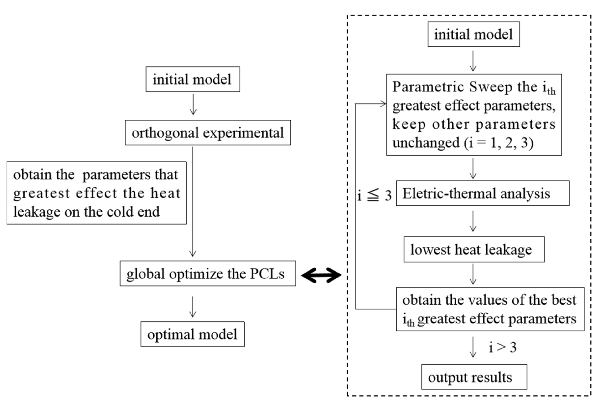
2.2. Optimization Procedure

Figure 3 is the flow chart of using orthogonal experiment to optimize the PCLs to achieve the minimum heat leakage. For this purpose, the optimization should experience two major steps: one is the orthogonal experiment, the other is the global optimization of the PCLs. Orthogonal experimental design is a design method to arrange and analyze multifactor experiments by using an orthogonal table [35]. It is carried out by selecting some representative factors among all experimental factors. Through the analysis of these experimental results, the overall situation of the test is understood, and the optimal factor is determined. The basic characteristic of orthogonal experimental design is to replace the comprehensive test with a partial test and to understand the situation of the comprehensive test through the analysis of partial test results. More information about orthogonal experimental design can be found in Ref. [35].
The specific optimization steps are as follows (Figure 3): First, orthogonal experiment is completed for the initial model. Thus, we obtain the parameters that have the greatest effect the heat leakage at the cold end. Then, we use these greatest effect factors to globally optimize the PCLs. The global optimization process is as follows: Based on the initial model, we choose the first three greatest effect parameters for a parametric sweep, keeping other parameters unchanged. Via the electric-thermal analysis, we can obtain the lowest heat leakage among the parametric sweep results. The corresponding value of the ith (i = 1, 2, 3) greatest effect parameter is the best one, so we change them and fix them in the next iteration. Then, we parametric sweep the second/third greatest effect parameters of the model and obtain the global lowest heat leakage. As with outputting a group of best dimensional parameters, the optimal model is achieved.

3. Results and Discussions

3.1. Results of 120 A Peltier Current Lead Optimization

3.1.1. Orthogonal Experimental Design for 120 A PCLs

For the chosen five optimized dimensional parameters, our orthogonal experiment considers their minimum and maximum values, as shown in Table 1. The principle for data selection is based on the previous literature [28,31,32,33] and our simulation experience. As there are five parameters, adding the ten parameters that describe the coupling effect between them, we design an L16 (215) orthogonal experimental table to achieve our goal. Here, the “L” represents the orthogonal table and the number “16” in subscript represents 16 lines, meaning the experiment with this orthogonal table contains 16 treatments. The base “2” in parentheses indicates the horizontal number of parameters. The exponent “15” in the parentheses indicates that there are 15 columns, and a maximum of 15 2-level parameters can be arranged using this orthogonal table. More information about orthogonal experimental design can be seen in Appendix A.1.

3.1.2. Orthogonal Experimental Results of 120 A PCLs

Table 2 is the orthogonal experimental results. The sample range indicates the influence weight of the corresponding parameters on the heat leakage of PCLs at the cold end. The larger the values, the greater the effect. From the sample range in Table 2, we can find that the most important factors affecting the heat leakage of PCLs at the cold end are D × E, B × C, and A. Here, the D × E and B × C indicate the parameters of coupling effect between D and E and between B and C, respectively. Furthermore, we find that parameter B (length of warm end copper leads) has little effect on the heat leakage at the cold end.
Moreover, the mean value 1 and mean value 2 indicates the influence of each level of parameters on the experimental indexes. As our goal is to achieve the minimum heat leakage of PCLs at the cold end, the smaller mean values correspond to better levels. Hence, for parameter A (copper leads radius r1), the level 1 (r1 = 3.0 mm) is better. Similarly, we obtain better values for L1 = 10.0 mm, L3 = 1500.0 mm, r2 = 30.0 mm, and L2 = 1.0 mm. We set these values as the initial values.

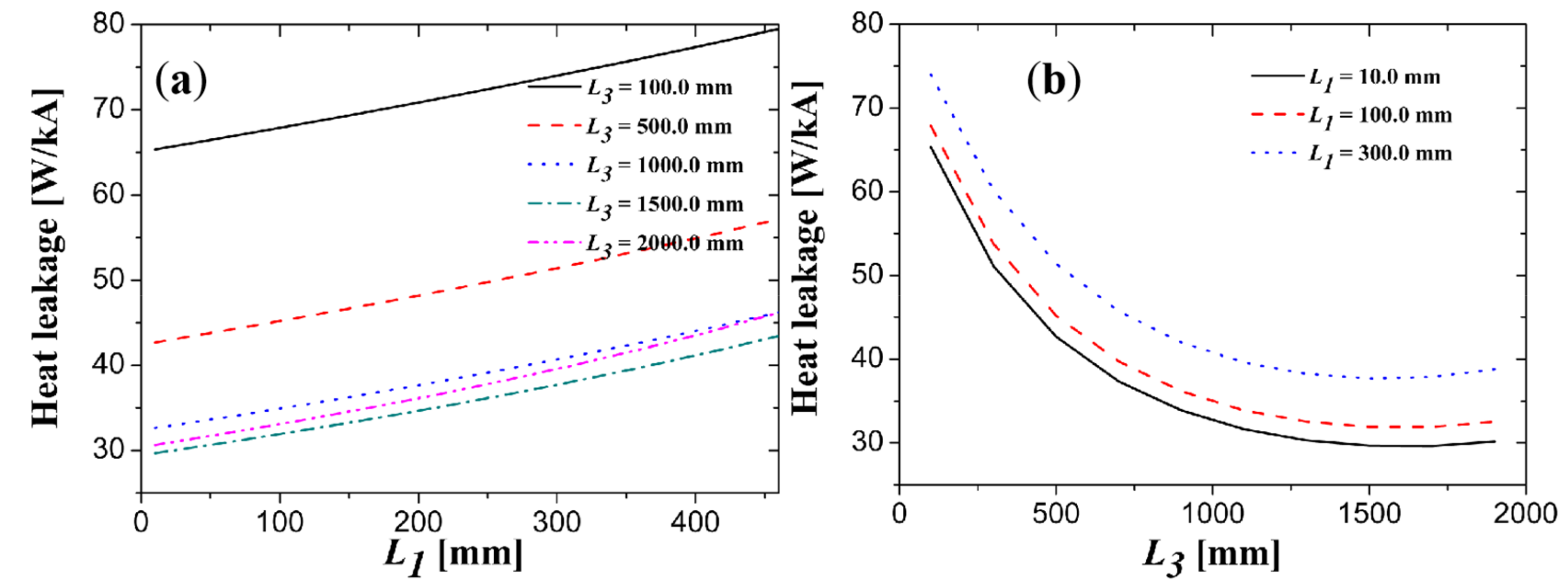
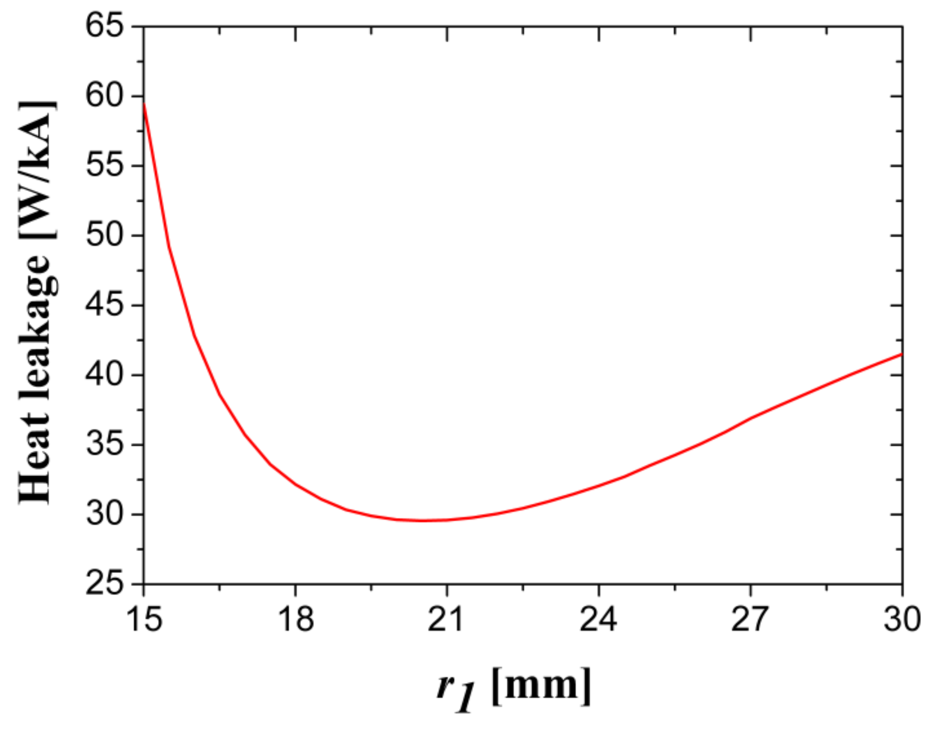
3.1.3. Global Optimization of the 120 A PCLs

Based on the orthogonal experimental results presented in the previous subsection, we know the parameters that have the greatest effect on the heat leakage at the cold end are D × E, B × C, and A. Thus, we first optimize the parameter of the interaction between D (radius of Bi2Te3, r2) and E (length of Bi2Te3, L2) to reveal their coupling influence on the heat leakage at the cold end (as shown in Figure 4), keeping the other parameters unchanged (radius of copper leads r1 = 3.0 mm, length of warm end copper leads L1 = 10.0 mm, length of cold end copper leads L3 = 1500.0 mm).
It can be seen in Figure 4a that using a smaller L2 achieves a smaller heat leakage value (black curve). Moreover, the value of r2 (radius of Bi2Te3) has a large influence on the heat leakage of PCLs. When the value of r2 is larger than a certain value (such as 10.0 mm), the heat leakage curve becomes stable at low values. In addition, from Figure 4b, we find that the heat leakage curves for r2 = 10.0 mm, 15.0 mm, and 20.0 mm are similar. Hence, we set the value of parameter D to r2 = 10.0 mm. Based on this setting, we obtain the lowest heat leakage of 35.49 W/kA at the cold end of PCLs when L2 = 1.0 mm. We set r2 equal to 10.0 mm and L2 equal 1.0 mm and fix them in the next iteration.
Then, we optimize the parameter of the interaction between B (L1) and C (L3) to reveal their coupling influence on the heat leakage at the cold end (as shown in Figure 5), keeping the other parameters unchanged (r1 = 3.0 mm, r2 = 10.0 mm, L2 = 1.0 mm). As shown in Figure 5a, the optimal value of cold end copper leads (L3) is some intermediate value, which is confirmed by Figure 5b. As shown in Figure 5b, with the increasing in the length of cold end copper leads (L3), the heat leakage curve is decreased first and then increased. Hence, we have best values for B and C (L1 = 10.0 mm, L3 = 700.0 mm). Under these optimization parameters, the lowest heat leakage at the cold end of PCLs is 30.1 W/kA.
Finally, we optimize the parameter A (radius of the copper leads r1), keeping the other parameters unchanged (L1 = 10.0 mm, L3 = 700.0 mm, r2 = 10.0 mm, L2 = 1.0 mm). Figure 6 illustrates the effect of r1 on the heat leakage of PCLs. Here, we obtain the best value for r1 = 3 mm and achieve an optimized structure of PCLs with the lowest heat leakage of 30.1 W/kA.
Then, we change the initial values for different dimensional parameters slightly, and through parametric sweep iteration, we obtain another two sets of optimal parameter sizes corresponding to a minimum heat leakage of PCLs, as shown in Table 3 (the details of the iteration progress are listed in Appendix A.2). Obviously, compared with the traditional copper current leads, the reduction rate of heat leakage at the cold end of PCLs exceeds 30%. That shows a huge advantage in saving energy for PCLs.
From Table 3, we find that the optimal value for r2 in the three cases is 10.0 mm. However, the value of r2 (radius of Bi2Te3) has a great influence on the heat leakage of PCLs. When the value of r2 is larger than a certain value (such as 10.0 mm), the heat leakage curve becomes stable at low values. Moreover, we find that the optimal value for L1 in the three cases is 10.0 mm. On the one hand, the orthogonal experimental results show that parameter B (L1) has little effect on the heat leakage at the cold end. On the other hand, through the parametric sweep iteration, we find that a shorter length of the warm end copper leads is better. Hence, we set the best value for L1 as 10.0 mm. Based on these settings, the optimal values of 120 A PCLs for L2 and L3 are increased with the increase in the radius of copper leads r1. In addition, the lowest heat leakage for three optimization cases is about 30.0 W/kA, which is in good agreement with previous works [28,31,32,33]. This indicates the method used in this work is reliable.
From these optimization processes, we find that the initial values have a great influence on the result. If change these optimal dimension parameters to the optimal ratio of L/A, there still exists a wide variety in the ratios of (L/A)p and (L/A)c. That is also consistent with previous studies [28,31,32,33], in which the optimal ratios of L/A were in a wide range. Hence, the problem of optimization of the PCLs is a multisolution problem.

3.2. Results of 1200 A Peltier Current Lead Optimization

3.2.1. Orthogonal Experimental Design for 1200 A PCLs

Considering the multiple uses of PCLs, designing a multiterminal current lead connector for higher current applications is necessary. We set the current in the multiterminal current lead connector as 1200 A. For the 1200 A PCL optimization, we also choose two values (the minimum and the maximum) for each optimized dimensional parameter, as shown in Table 4. The principle for data selection is based on ensuring the convergence of the model, choosing a parameter value range as wide as possible. We also design an L16 (215) orthogonal experimental table to achieve our goal. More information about orthogonal experimental design can be seen in Appendix A.3.

3.2.2. Orthogonal Experimental Results of 1200 A PCLs

Table 5 is the orthogonal experimental results. As the larger value of the sample range indicates the greater effect of the corresponding parameters on the heat leakage of PCLs at the cold end, we can summarize the following effect weight order: D × E, D, E, B × C, and A. To some extent, it is consistent with the order D × E, B × C, and A, which is that found in the orthogonal experimental results for the 120 A PCLs. Furthermore, for the optimization of 1200 A PCLs, parameter B (length of warm end copper leads) also has little effect on the heat leakage at the cold end. As the mean value is smaller, the corresponding level is better. For parameter A (copper leads radius r1), the level 1 (r1 = 10.0 mm) is better. Similarly, we have better values for L1 = 10.0 mm, L3 = 1500.0 mm, r2 = 50.0 mm, and L2 = 1.0 mm. The chosen levels for all these parameters are consistent with the orthogonal experimental results for 120 A PCLs. We set these values as the initial values.

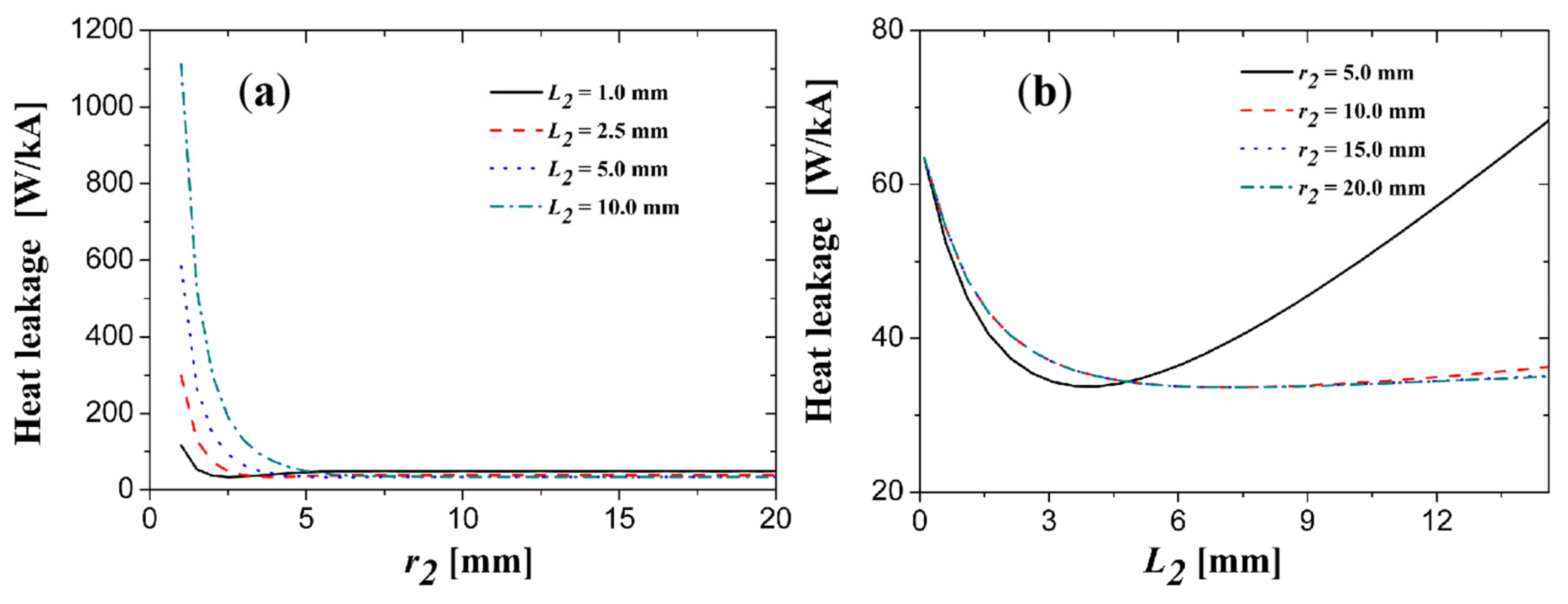
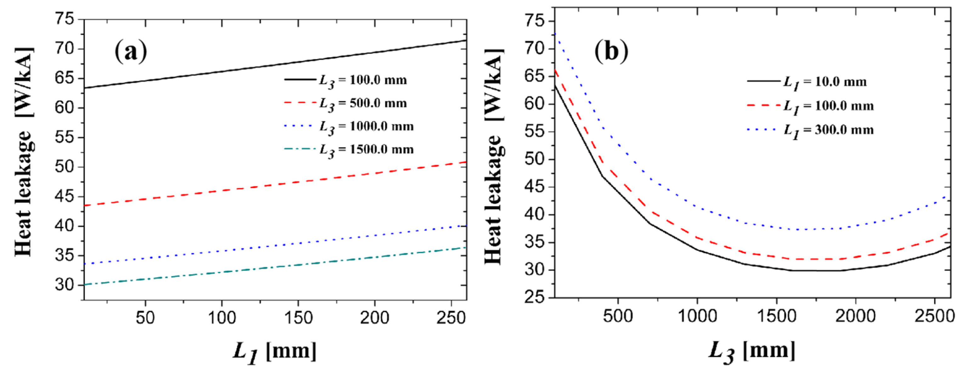
3.2.3. Global Optimization of the 1200 A PCLs

Based on the orthogonal experimental results presented in the previous subsection, we choose the first three greatest parameters to optimize. Through parametric sweep iteration, by changing the initial values for different dimensional parameters slightly, we obtain several sets of optimal parameter sizes corresponding to a minimum heat leakage of PCLs, as shown in Table 6. Obviously, compared with the traditional copper current leads, the reduction rate of heat leakage at the cold end of 1200 A PCLs is 30%. That shows a huge advantage in saving energy for PCLs. The details of the iteration progress are listed in Appendix A.4.
From Table 6 we find that the optimal values for r2 in the three cases are 15.0 mm, 20.0 mm, and 30.0 mm, which are a little larger than the radius of copper leads. Through the optimization process (A4), we know that though the value of r2 (radius of Bi2Te3) has a great influence on the heat leakage of PCLs; when the value of r2 is larger than a certain value (such as 15.0 mm, 20.0 mm, or 30.0 mm), the heat leakage curve will become stable at low values. Based on these considerations, the optimal values for r2 are selected as 15.0 mm, 20.0 mm, and 30.0 mm. Moreover, the optimal value for L1 in the three cases is 10.0 mm. The reason is the same as for 120 A PCLs. Based on these settings, the optimal values of 1200 A PCLs for L2 and L3 are also increased with the increase in the radius of copper leads r1. Furthermore, the problem of optimization of the 1200 A PCLs is also a multisolution problem, where there exists a wide variety in the optimal ratios of (L/A)p and (L/A)c.
The lowest heat leakage found for 1200 A PCLs, nearly 30.0 W/kA, is at the same level as that found for 120 A PCLs. This indicates that the heat leakage for a multiterminal current lead connector with a total current of 1200 A is equal to that of a single PCL with a current of 1200 A. When taking the heat dissipation area at the hot end into account, multiterminal solutions are better solutions for kiloampere current leads.

4. Conclusions

Through a COMSOL two-dimensional axisymmetric model of PCL finite element simulation, this study first used the orthogonal experiment to scientifically choose the parameters that have a great influence on the heat leakage at the cold end. Through our simulation, we firstly found that the coupling effect between the radius of Bi2Te3 (r2) and the length of Bi2Te3 (L2) has the greatest effect on the heat leakage of PCLs at the cold end for 120 A and 1200 A PCLs. The second and third factors for 120 A PCLs are the coupling effect between the length of warm end and cold end copper (L1 × L3) and the radius of copper (r1), respectively. For 1200 A PCLs, the second and third factors are the radius of Bi2Te3 (r2) and the length of Bi2Te3 (L2), respectively.
Based on these more influential parameters, the optimization range was narrowed. Through parametric sweep iteration, by changing the initial values for different dimensional parameters slightly, we obtained several sets of optimal parameter sizes. We found that the problem of optimization of the 120 A and 1200 A PCLs is a multisolution problem, where there exists a wide variety in the optimal ratios of (L/A)p and (L/A)c. Therefore, in the practical application design, it is more necessary to consider the important factors affecting the heat leakage at the cold end (r2 × L2, L1 × L3, r1).
Through our calculation comparison, we determined that the lowest cold end leakage heat for PCLs of 120 A and 1200 A is close to 30.0 W/kA. This indicates that the heat leakage for a multiterminal current lead connector with a total current of 1200 A is equal to that of a single PCL with a current of 1200 A. When taking the heat dissipation area on the hot end into account, multiterminal solutions are better solutions for kiloampere current leads. The method developed in this work significantly reduces the number of simulation cases and improves the comprehensiveness of optimal solutions. This method can be used to optimize HTS current leads with more complex structures and materials to reduce overall heat leakage, which deserves future work.

Author Contributions

S.Z. and S.D. contributed to the overall study design and analysis. L.L. (Linying Liu) contributed to computer simulation and writing of the manuscript. S.Z., S.D., L.L. (Lingfeng Lai), and C.G. provided technical support and revised the manuscript. S.Z. and L.L. (Linying Liu) provided funding acquisition. All authors have read and agreed to the published version of the manuscript.

Funding

This work was supported in part by the National Science Foundation of China under Grant 51807192 and in part by the China Post Doctoral Science Foundation under Grant 2020M671917.

Conflicts of Interest

The authors declare no conflict of interest.

Appendix A

Appendix A.1. Orthogonal Experimental Schedule for 120 A PCLs

Before solving the optimization problems, we usually need to choose a suitable orthogonal table. Based on the number and level of the parameter factors, we need to design the header of the orthogonal table. Then, we carry out the orthogonal experiment. More information about orthogonal experimental design can be found in [35]. Table A1 is the orthogonal experimental schedule for the 120 A PCLs, which is a very important intermediate process for the orthogonal experiment.
Table A1. Orthogonal experimental schedule for 120 A PCLs.
Column Number124815
ParametersA: Copper Leads Radius (r1/mm)B: Length of Warm end Copper Leads (L1/mm)C: Length of Cold End Copper Leads (L3/mm)D: Radius of Bi2Te3 (r2/mm)E: Length of Bi2Te3 (L2/mm)Simulation Results (W/kA)
Simulation 13.010.0100.01.01.0154.9
Simulation 23.010.0100.030.030.076.1
Simulation 33.010.01500.01.030.01608.3
Simulation 43.010.01500.030.01.0158.8
Simulation 53.0300.0100.01.030.04920.0
Simulation 63.0300.0100.030.01.074.1
Simulation 73.0300.01500.01.01.0384.7
Simulation 83.0300.01500.030.030.0351.9
Simulation 930.010.0100.01.030.05676.9
Simulation 1030.010.0100.030.01.05816.0
Simulation 1130.010.01500.01.01.0178.6
Simulation 1230.010.01500.030.030.0215.8
Simulation 1330.0300.0100.01.01.0183.9
Simulation 1430.0300.0100.030.030.0244.6
Simulation 1530.0300.01500.01.030.05507.5
Simulation 1630.0300.01500.030.01.01066.6

Appendix A.2. Global Optimization of the PCLs for 120 A PCLs

Appendix A.2.1. The Simulation Case 2 for 120 A PCLs

Based on the orthogonal experimental results in Section 3.1.2, we know the first set of parameters that have the greatest effect on the heat leakage at the cold end is D × E, B × C, and A. Thus, we first optimize the parameter of the interaction between D (radius of Bi2Te3, r2) and E (length of Bi2Te3, L2) to reveal their coupling influence on the heat leakage at the cold end (as shown in Figure A1), keeping the other parameters unchanged (radius of copper leads r1 = 3.0 mm, length of warm end copper leads L3 = 10.0 mm, length of cold end copper leads L1 = 1000.0 mm).
Then, we change the initial values for different dimensional parameters slightly, and through parametric sweep iteration, we obtain another two sets of optimal parameter sizes corresponding to a minimum heat leakage of PCLs, as shown in Figure A1, Figure A2 and Figure A3 and Figure A4, Figure A5 and Figure A6, respectively.
Figure A1. Iteration step 1: the coupling influence between D (r2) and E (L2) on the cold end heat leakage of PCLs (keeping parameters r1 = 4.0 mm, L1 = 10.0 mm, L3 = 1500.0 mm unchanged; in this iteration Qmin = 30.0 W/kA). (a) The heat leakage vary with D (r2); (b)The heat leakage vary with E (L2).
Electronics 10 01054 g0a1
Figure A2. Iteration step 2: the coupling influence between B (L1) and C (L3) on the cold end heat leakage of PCLs (keeping parameters r1 = 4.0 mm, r2 = 10.0 mm, L2 = 3.5 mm unchanged; in this iteration Qmin = 29.7 W/kA). (a) The heat leakage vary with B (L1); (b)The heat leakage vary with C (L3).
Electronics 10 01054 g0a2
Figure A3. Iteration step 3: the effect of radius of the copper leads r1 on the cold end heat leakage of PCLs (keeping parameters L1 = 10.0 mm, L3 = 1100.0 mm, r2 = 10.0 mm, L2 = 3.5 mm unchanged; in this iteration Qmin = 29.7 W/kA).
Electronics 10 01054 g0a3

Appendix A.2.2. The Simulation Case 3 for 120 A PCLs

Figure A4. Iteration step 1: the coupling influence between D (r2) and E (L2) on the cold end heat leakage of PCLs (keeping parameters r1 = 5.0 mm, L1 = 10.0 mm, L3 = 1500.0 mm unchanged; in this iteration Qmin = 33.6 W/kA). (a) The heat leakage vary with D (r2); (b)The heat leakage vary with E (L2).
Electronics 10 01054 g0a4
Figure A5. Iteration step 2: the coupling influence between B (L1) and C (L3) on the cold end heat leakage of PCLs (keeping parameters r1 = 5.0 mm, r2 = 10.0 mm, L2 = 7.0 mm unchanged, in this iteration Qmin = 29.9 W/kA). (a) The heat leakage vary with B (L1); (b)The heat leakage vary with C (L3).
Electronics 10 01054 g0a5
Figure A6. Iteration step three: the effect of radius of the copper leads r1 on the cold end heat leakage of PCLs (keeping parameters L1 = 10.0 mm, L3 = 1900.0 mm, r2 = 10.0 mm, L2 = 7.0 mm unchanged; in this iteration Qmin = 29.8 W/kA).
Electronics 10 01054 g0a6

Appendix A.3. Orthogonal Experimental Schedule for 1200 A PCLs

Table A2 is the orthogonal experimental schedule for the 1200 A PCLs, which is a very important intermediate process for the orthogonal experiment.
Table A2. Orthogonal experimental schedule for 1200 A PCLs.
Column Number124815
ParametersA: Copper Leads Radius (r1/mm)B: Length of Warm End Copper Leads (L1/mm)C: Length of Cold End Copper Leads (L3/mm)D: Radius of Bi2Te3 (r2/mm)E: Length of Bi2Te3 (L2/mm)Simulation Results (W/kA)
Simulation 110.010.0100.05.01.069.7
Simulation 210.010.0100.050.050.0196.5
Simulation 310.010.01500.05.050.01254.7
Simulation 410.010.01500.050.01.068.6
Simulation 510.0300.0100.05.050.03482.7
Simulation 610.0300.0100.050.01.074.0
Simulation 710.0300.01500.05.01.0304.4
Simulation 810.0300.01500.050.050.0357.8
Simulation 980.010.0100.05.050.03774.3
Simulation 1080.010.0100.050.01.01845.0
Simulation 1180.010.01500.05.01.078.6
Simulation 1280.010.01500.050.050.063.2
Simulation 1380.0300.0100.05.01.083.0
Simulation 1480.0300.0100.050.050.067.5
Simulation 1580.0300.01500.05.050.03617.8
Simulation 1680.0300.01500.050.01.0612.8

Appendix A.4. Global Optimization of the PCLs for 1200 A PCLs

Appendix A.4.1. The Simulation Case 1 for 1200 A PCLs

Based on the orthogonal experimental results in Section 3.2.2, we know the first set of parameters that have the greatest effect on the heat leakage at the cold end is D × E, D, E, B × C, and A. To some extent, this is consistent with the order of orthogonal experimental results for the 120 A PCLs: D × E, B × C, and A. Thus, we first optimize the parameter of the interaction between D (radius of Bi2Te3, r2) and E (length of Bi2Te3, L2) to reveal their coupling influence on the heat leakage at the cold end (as shown in Figure A7), keeping the other parameters unchanged (radius of copper leads r1 = 10.0 mm, length of warm end copper leads L1 = 100.0 mm, length of cold end copper leads L3 = 500.0 mm).
Figure A7. The coupling influence between D (r2) and E (L2) on the cold end heat leakage of PCLs. (a) The heat leakage vary with D (r2); (b)The heat leakage vary with E (L2).
Electronics 10 01054 g0a7
It can be seen in Figure A7a that the use of a smaller L2 leads to achieving a smaller heat leakage value (black curve). From Figure A7b, we find that if r2 ≥ 15.0 mm, the heat leakage curves are similar. Hence, we set the value of parameters D and E (r2 = 15.0 mm, L2 = 1.6 mm) and fix them in the next iteration. For the first iteration, the lowest heat leakage at the cold end of PCLs is 37.2 W/kA.
Then, we optimize the parameter of the interaction between B (L1) and C (L3) to reveal their coupling influence on the heat leakage at the cold end (as shown in Figure A8), keeping the other parameters unchanged (r1 = 10.0 mm, r2 = 15.0 mm, L2 = 1.6 mm). As shown in Figure A8a, the optimal value of cold end copper leads (L3) is some intermediate value, which is confirmed by Figure A8b. With the increase in the length of cold end copper leads (L3), the heat leakage curve is decreased first and then increased (Figure A8b). Hence, we obtain the best values for B and C (L1 = 10.0 mm, L3 = 700.0 mm). Under these optimization parameters, the lowest heat leakage at the cold end of PCLs is 29.9 W/kA.
Figure A8. The coupling influence between B (L1) and C (L3) on the cold end heat leakage of PCLs. (a) The heat leakage vary with B (L1); (b)The heat leakage vary with C (L3).
Electronics 10 01054 g0a8
Finally, we optimize the parameter A (radius of the copper leads r1), keeping the other parameters unchanged (L1 = 10.0 mm, L3 = 700.0 mm, r2 = 15.0 mm, L2 = 1.6 mm). Figure A9 illustrates the effect of r1 on the heat leakage of PCLs. Here, we obtain the best value for r1 = 10.0 mm and achieve an optimized structure of PCLs with the lowest heat leakage of 29.9 W/kA.
Figure A9. The effect of radius of the copper leads r1 on the cold end heat leakage of PCLs.
Electronics 10 01054 g0a9
Then, we change the initial values for different dimensional parameters slightly, and through parametric sweep iteration, we obtain another two sets of optimal parameter sizes corresponding to a minimum heat leakage of PCLs, as shown in Figure A10, Figure A11 and Figure A12 and Figure A13, Figure A14 and Figure A15, respectively.

Appendix A.4.2. The Simulation Case 2 for 1200 A PCLs

Based on the orthogonal experimental results presented in Section 3.2.2, we know the set of parameters that have the greatest effect on the heat leakage at the cold end is D × E, D, E, B × C, and A. Thus, we first optimize the parameter of the interaction between D (radius of Bi2Te3, r2) and E (length of Bi2Te3, L2) to reveal their coupling influence on the heat leakage at the cold end (as shown in Figure A10), keeping the other parameters unchanged (radius of copper leads r1 = 15.0 mm, length of warm end copper leads L1 = 100.0 mm, length of cold end copper leads L3 = 1500.0 mm).
Figure A10. Iteration step one: the coupling influence between D (r2) and E (L2) on the cold end heat leakage of PCLs (keeping parameters r1 = 15.0 mm, L1 = 100.0 mm, L3 = 1500.0 mm unchanged; in this iteration Qmin = 34.9W/kA). (a) The heat leakage vary with D (r2); (b)The heat leakage vary with E (L2).
Electronics 10 01054 g0a10
Then, we optimize the parameter of the interaction between B (L1) and C (L3) to reveal their coupling influence on the heat leakage at the cold end (as shown in Figure A11), keeping the other parameters unchanged (r1 = 15.0 mm, r2 = 20.0 mm, L2 = 3.5 mm). As shown in Figure A11, we obtain the best values for B and C (L1 = 10.0 mm, L3 = 1700.0 mm). Under these optimization parameters, the lowest heat leakage at the cold end of PCLs is 29.6 W/kA.
Finally, we optimize the parameter A (radius of the copper leads r1), keeping the other parameters unchanged (L1 = 10.0 mm, L3 = 1700.0 mm, r2 = 20.0 mm, L2 = 3.5 mm). Figure A12 illustrates the effect of r1 on the heat leakage of PCLs. Here, we obtain the best value for r1 = 15.5 mm and achieve an optimized structure of PCLs with the lowest heat leakage of 29.6 W/kA.
Figure A11. Iteration step two: the coupling influence between B (L1) and C (L3) on the cold end heat leakage of PCLs (keeping parameters r1 = 15.0 mm, r2 = 20.0 mm, L2 = 3.5 mm unchanged; in this iteration Qmin = 29.6 W/kA). (a) The heat leakage vary with B (L1); (b)The heat leakage vary with C (L3).
Electronics 10 01054 g0a11
Figure A12. Iteration step three: the effect of radius of the copper leads r1 on the cold end heat leakage of PCLs (keeping parameters L1 = 10.0 mm, L3 = 1700.0 mm, r2 = 20.0 mm, L2 = 3.5 mm unchanged; in this iteration Qmin = 29.6 W/kA).
Electronics 10 01054 g0a12

Appendix A.4.3. The Simulation Case 3 for 1200 A PCLs

Based on the orthogonal experimental results presented in Section 3.2.2, we know the set of parameters that have the greatest effect on the heat leakage at the cold end is D × E, D, E, B × C, and A. Thus, we first optimize the parameter of the interaction between D (radius of Bi2Te3, r2) and E (length of Bi2Te3, L2) to reveal their coupling influence on the heat leakage at the cold end (as shown in Figure A13), keeping the other parameters unchanged (radius of copper leads r1 = 20.0 mm, length of warm end copper leads L1 = 100.0 mm, length of cold end copper leads L3 = 1500.0 mm).
Figure A13. Iteration step one: the coupling influence between D (r2) and E (L2) on the cold end heat leakage of PCLs (keeping parameters r1 = 20.0 mm, L1 = 100.0 mm, L3 = 1500.0 mm unchanged; in this iteration Qmin = 35.7 W/kA). (a) The heat leakage vary with D (r2); (b)The heat leakage vary with E (L2).
Electronics 10 01054 g0a13
Then, we optimize the parameter of the interaction between B (L1) and C (L3) to reveal their coupling influence on the heat leakage at the cold end (as shown in Figure A14), keeping the other parameters unchanged (r1 = 20.0 mm, r2 = 30.0 mm, L2 = 7.5 mm). As shown in Figure A14, we obtain the best values for B and C (L1 = 10.0 mm, L3 = 2900.0 mm). Under these optimization parameters, the lowest heat leakage at the cold end of PCLs is 29.9 W/kA.
Finally, we optimize the parameter A (radius of the copper leads r1), keeping the other parameters unchanged (L1 = 10.0 mm, L3 = 2900.0 mm, r2 = 30.0 mm, L2 = 7.5 mm). Figure A15 illustrates the effect of r1 on the heat leakage of PCLs. Here, we obtain the best value for r1 = 20.0 mm and achieve an optimized structure of PCLs with the lowest heat leakage of 29.8 W/kA.
Figure A14. Iteration step two: the coupling influence between B (L1) and C (L3) on the cold end heat leakage of PCLs (keeping parameters r1 = 20.0 mm, r2 = 30.0 mm, L2 = 7.5 mm unchanged; in this iteration Qmin = 29.8 W/kA). (a) The heat leakage vary with B (L1); (b)The heat leakage vary with C (L3).
Electronics 10 01054 g0a14
Figure A15. Iteration step three: the effect of radius of the copper leads r1 on the cold end heat leakage of PCLs (keeping parameters L1 = 10.0 mm, L3 = 2900.0 mm, r2 = 30.0 mm, L2 = 7.5 mm unchanged; in this iteration Qmin = 29.8 W/kA).
Electronics 10 01054 g0a15

References

  1. Dai, S.; Xiao, L.; Zhang, H.; Teng, Y.; Liang, X.; Song, N.; Cao, Z.; Zhu, Z.; Gao, Z.; Ma, T.; et al. Testing and Demonstration of a 10-kA HTS DC Power Cable. IEEE Trans. Appl. Supercond. 2014, 24, 99–102. [Google Scholar]
  2. Yamaguchi, S.; Koshizuka, H.; Hayashi, K.; Sawamura, T. Concept and Design of 500 Meter and 1000 Meter DC Superconducting Power Cables in Ishikari. IEEE Trans. Appl. Supercond. 2015, 25, 5402504. [Google Scholar] [CrossRef]
  3. Yang, B.; Kang, J.; Lee, S.; Choi, C.; Moon, Y. Qualification Test of a 80 kV 500 MW HTS DC Cable for Applying Into Real Grid. IEEE Trans. Appl. Supercond. 2015, 25, 5402705. [Google Scholar] [CrossRef]
  4. Sytnikov, V.E.; Bemert, S.E.; Krivetsky, I.V.; Karpov, V.N.; Romashov, M.A.; Shakarian, Y.G.; Nosov, A.A.; Fetisov, S.S. The Test Results of AC and DC HTS Cables in Russia. IEEE Trans. Appl. Supercond. 2016, 26, 5401304. [Google Scholar] [CrossRef]
  5. Xie, W.; Wei, B.G.; Yao, Z.F. Introduction of 35 kV km Level Domestic Second Generation High Temperature Superconducting Power Cable Project in Shanghai, China. J. Supercond. Nov. Magn. 2020, 33, 1927–1931. [Google Scholar] [CrossRef]
  6. Lee, C.; Son, H.; Won, Y.; Kim, Y.; Ryu, C.; Park, M.; Iwakuma, M. Progress of the First Commercial Project of High-Temperature Superconducting Cables by KEPCO in Korea. Supercond. Sci. Technol. 2020, 33, 44006. [Google Scholar] [CrossRef]
  7. Doukas, D.I. Superconducting Transmission Systems: Review, Classification, and Technology Readiness Assessment. IEEE Trans. Appl. Supercond. 2019, 29, 5401205. [Google Scholar] [CrossRef]
  8. Chen, W.; Song, P.; Jiang, H.; Zhu, J.H.; Zou, S.N.; Qu, T.M. Investigations on Quench Recovery Characteristics of High-Temperature Superconducting Coated Conductors for Superconducting Fault Current Limiters. Electronics 2021, 10, 259. [Google Scholar] [CrossRef]
  9. Hong, Z.; Sheng, J.; Yao, L.; Gu, J.; Jin, Z. The Structure, Performance and Recovery Time of a 10 kV Resistive Type Superconducting Fault Current Limiter. IEEE Trans. Appl. Supercond. 2013, 23, 5601304. [Google Scholar]
  10. Qiu, Q.Q.; Xiao, L.Y.; Zhang, J.Y.; Zhang, Z.F.; Song, N.H.; Jing, L.W.; Zha, W.H.; Du, X.J.; Teng, Y.P.; Zhou, Z.H.; et al. Design and Test of 40-kV/2-kA DC Superconducting Fault Current Limiter. IEEE Trans. Appl. Supercond. 2020, 30, 2988068. [Google Scholar] [CrossRef]
  11. Dai, S.T.; Ma, T.; Xue, C.; Zhao, L.Q.; Huang, Y.; Hu, L.; Wang, B.Z.; Zhang, T.; Xu, X.F.; Cai, L.L.; et al. Development and Test of a 220 kV/1.5 kA Resistive Type Superconducting Fault Current Limiter. Phys. C 2019, 565, 1253501. [Google Scholar] [CrossRef]
  12. Hao, L.N.; Huang, Z.; Dong, F.L.; Qiu, D.R.; Shen, B.Y.; Jin, Z.J. Study on Electrodynamic Suspension System with High-Temperature Superconducting Magnets for a High-Speed Maglev Train. IEEE Trans. Appl. Supercond. 2019, 29, 3600105. [Google Scholar] [CrossRef]
  13. Lee, H.W.; Kim, K.C.; Lee, J. Review of maglev train technologies. IEEE Trans. Magn. 2006, 42, 1917–1925. [Google Scholar]
  14. Deng, Z.G.; Zhang, W.H.; Zheng, J.; Wang, B.; Ren, Y.; Zheng, X.X.; Zhang, J.H. A High-Temperature Superconducting Maglev-Evacuated Tube Transport (HTS Maglev-ETT) Test System. IEEE Trans. Appl. Supercond. 2017, 27, 3602008. [Google Scholar] [CrossRef]
  15. Deng, Z.G.; Zhang, W.H.; Zheng, J.; Ren, Y.; Jiang, D.H.; Zheng, X.X.; Zhang, J.H.; Gao, P.F.; Lin, Q.X.; Song, B.; et al. A High-Temperature Superconducting Maglev Ring Test Line Developed in Chengdu, China. IEEE Trans. Appl. Supercond. 2016, 26, 3602408. [Google Scholar] [CrossRef]
  16. Wang, Y.; Chan, W.K.; Schwartz, J. Self-Protection Mechanisms in No-Insulation (RE) Ba2Cu3Ox High Temperature Superconductor Pancake Coils. Supercond. Sci. Technol. 2016, 29, 45007. [Google Scholar] [CrossRef]
  17. Wang, Y.W.; Weng, F.J.; Li, J.W.; Souc, J.; Gomory, F.; Zou, S.N.; Zhang, M.; Yuan, W.J. No-Insulation High-Temperature Superconductor Winding Technique for Electrical Aircraft Propulsion. IEEE Trans. Transp. Electrif. 2020, 6, 1613–1624. [Google Scholar] [CrossRef]
  18. Jun, Z.; Feng, X.; Wei, C.; Yijun, D.; Jin, C.; Wenbin, T. The Study and Test for 1MW High Temperature Superconducting Motor. IEEE/CSC ESAS Eur. Supercond. News Forum 2013, 23, 6–9. [Google Scholar]
  19. Gamble, B.; Snitchler, G.; MacDonald, T. Full Power Test of a 36.5 MW HTS Propulsion Motor. IEEE Trans. Appl. Supercond. 2010, 21, 1083–1088. [Google Scholar] [CrossRef]
  20. Sivasubramaniam, K.; Zhang, T.; Lokhandwalla, M.; Laskaris, E.; Bray, J.; Gerstler, B.; Shah, M.; Alexander, J. Development of a High Speed HTS Generator for Airborne Applications. IEEE Trans. Appl. Supercond. 2009, 19, 1656–1661. [Google Scholar] [CrossRef]
  21. Song, X.; Bührer, C.; Brutsaert, P.; Krause, J.; Ammar, A.; Wiezoreck, J.; Hansen, J.; Rebsdorf, A.V.; Dhalle, M.; Bergen, A. Designing and Basic Experimental Validation of the World’s First MW-Class Direct-Drive Superconducting Wind Turbine Generator. IEEE Trans. Energy Convers. 2019, 34, 2218–2225. [Google Scholar] [CrossRef]
  22. Filipenko, M.; Kühn, L.; Gleixner, T.; Thummet, M.; Lessmann, M.; Möller, D.; Böhm, M.; Schröter, A.; Häse, K.; Grundmann, J. Concept Design of a High Power Superconducting Generator for Future Hybrid-Electric Aircraft. Supercond. Sci. Technol. 2020, 33, 054002. [Google Scholar] [CrossRef]
  23. Komiya, M.; Aikawa, T.; Sasa, H.; Miura, S.; Iwakuma, M.; Yoshida, T.; Sasayama, T.; Tomioka, A.; Konno, M.; Izumi, T. Design Study of 10 MW REBCO Fully Superconducting Synchronous Generator for Electric Aircraft. IEEE Trans. Appl. Supercond. 2019, 29, 5204306. [Google Scholar] [CrossRef]
  24. Seifert, W.; Ueltzen, M.; Muller, E. One-Dimensional Modelling of Thermoelectric Cooling. Phys. Status Solidi A Appl. Mat. 2002, 194, 277–290. [Google Scholar] [CrossRef]
  25. Sato, K.; Okumura, H.; Yamaguchi, S. Numerical Calculations for Peltier Current Lead Designing. Cryogenics 2001, 41, 497–503. [Google Scholar] [CrossRef]
  26. Xiangchun, X. On the Optimal Design of Gas-Cooled Peltier Current Leads. IEEE Trans. Appl. Supercond. 2003, 13, 48–53. [Google Scholar] [CrossRef]
  27. Jeong, E.S. Optimization of Conduction-Cooled Peltier Current Leads. Cryogenics 2005, 45, 516–522. [Google Scholar] [CrossRef]
  28. Chen, G.; Wang, Y.; Pi, W.; Shi, C.; Li, T.; Li, J.; Zhang, H. Experimental Investigation on 100 A-Class PCL for DC HTS Devices. IEEE Trans. Appl. Supercond. 2016, 26, 4800805. [Google Scholar] [CrossRef]
  29. Michael, P.C.; Galea, C.A.; Bromberg, L. Cryogenic Current Lead Optimization Using Peltier Elements and Configurable Cooling. IEEE Trans. Appl. Supercond. 2015, 25, 4801805. [Google Scholar] [CrossRef]
  30. Miyata, S.; Yoshiwara, Y.; Watanabe, H.; Yamauchi, K.; Makino, K.; Yamaguchi, S. Evaluation of Thermoelectric Performance of Peltier Current Leads Designed for Superconducting Direct-Current Transmission Cable Systems. IEEE Trans. Appl. Supercond. 2016, 26, 5401604. [Google Scholar] [CrossRef]
  31. Dai, S.; Liu, M.; Ma, T.; Zhang, T.; Hu, L.; Wang, B.; Wang, Y. Experimental Study on Heat-leakage of 100 A-Class PCL with Varying Cross Section. IEEE Trans. Appl. Supercond. 2019, 29, 4800104. [Google Scholar] [CrossRef]
  32. Chen, G.; Wang, Y.; Pi, W.; Kan, C.; Fu, Y.; Shi, C.; Li, T.; Li, J. Heat Leakage Analysis on Peltier Current Leads of Different Structures. IEEE Trans. Appl. Supercond. 2016, 26, 8801504. [Google Scholar] [CrossRef]
  33. Liu, M.; Wang, Y.; Dai, S.; Wang, J.; Peng, C.; Chen, H.; Jiang, Z.; Hu, Y. Experimental Study on 1 kA-Class Peltier Current Lead for Superconducting DC Devices. IEEE Trans. Appl. Supercond. 2019, 29, 4802504. [Google Scholar] [CrossRef]
  34. COMSOL. COMSOL Multiphysics®, v.5.3. 2017. Available online: https://www.comsol.com/release/5.3 (accessed on 15 April 2021).
  35. Hicks, C.R. Fundamental Concepts in the Design of Experiments, 4th ed.; Oxford University Press: Oxford, UK, 1993. [Google Scholar]
Figure 1. Schematic view of a PCL.
Electronics 10 01054 g001
Figure 2. Schematic view of a simplified PCL.
Electronics 10 01054 g002
Figure 3. Global optimization procedure.
Electronics 10 01054 g003
Figure 4. The coupling influence between D (r2) and E (L2) on the cold end heat leakage of PCLs. (a) The heat leakage vary with D (r2); (b)The heat leakage vary with E (L2).
Electronics 10 01054 g004
Figure 5. The coupling influence between B (L1) and C (L3) on the cold end heat leakage of PCLs. (a) The heat leakage vary with B (L1); (b)The heat leakage vary with C (L3).
Electronics 10 01054 g005
Figure 6. The effect of radius of the copper leads r1 on the cold end heat leakage of PCLs.
Electronics 10 01054 g006
Table 1. Orthogonal experimental design for 120 A PCLs.
SymbolQuantityValues (mm)Column Number
Level 1Level 2
A: r1Radius of copper leads3.030.01
B: L1Length of warm end copper leads10.0300.02
C: L3Length of cold end copper leads100.01500.04
D: r2Radius of Bi2Te31.030.08
E: L2Length of Bi2Te31.030.015
Table 2. Orthogonal experimental results of 120 A PCLs.
Column Number123456789101112131415
ParametersA: Copper Leads Radius (r1/mm)B: Length of Warm end Copper Leads (L1/mm)A × BC: Length of Cold End Copper Leads (L3/mm)A × CB × CD × ED: Radius of Bi2Te3 (r2/mm)A × DB × DC × EC × DB × EA × EE: Length of Bi2Te3 (L2/mm)
Mean value 1966.01736.5 11125.02143.21524.12379.2223.72326.71801.21169.41738.91591.02166.41552.01002.1
Mean value 22361.21591.62202.31184.01803.1948.03103.51000.51526.02157.81588.31736.21160.81775.12325.1
Sample range1395.3143.91077.3959.2279.11431.22879.81326.2275.3988.5150.6145.31005.6223.21323.1
1 While the orthogonal experimental results indicate the better initial value for L1 is 300.0 mm, we choose L1 = 10.0 mm as the initial value. On the one hand, there exists a small difference between the Mean values 1 and 2 for L1 in Table 2, but this difference provides insufficient support to choose which one is better. On the other hand, through the parametric sweep iteration, we find that a shorter length of warm end copper leads is better. In addition, the orthogonal experimental results indicate that the parameter B (L1) has little effect on the heat leakage at the cold end. Based on these considerations, we choose L1 = 10.0 mm as the initial value.
Table 3. Three sets of optimal parameters for 120 A PCLs.
SymbolQuantityOptimized Parameters
Case 1Case 2Case 3
A: r1Radius of copper leads (mm)3.04.05.5
B: L1Length of warm end copper leads (mm)10.010.010.0
C: L3Length of cold end copper leads (mm)700.01100.01900.0
D: r2Radius of Bi2Te3 (mm)10.010.010.0
E: L2Length of Bi2Te3 (mm)1.03.57.0
Lowest heat leakage (W/kA)30.129.729.8
Heat leakage with pure copper (W/kA)43.245.647.9
Reduction rate of cold end heat leakage30.4%34.8%37.7%
Table 4. Orthogonal experimental design for 1200 A PCLs.
SymbolQuantityValues (mm)Column Number
Level 1Level 2
A: r1Radius of Copper leads10.080.01
B: L1Length of warm end copper leads10.0300.02
C: L3Length of cold end copper leads100.01500.04
D: r2Radius of Bi2Te35.050.08
E: L2Length of Bi2Te31.050.015
Table 5. Orthogonal experimental results of 1200 A PCLs.
Column Number123456789101112131415
ParametersA: Copper Leads Radius (r1/mm)B: Length of Warm End Copper Leads (L1/mm)A × BC: Length of Cold end Copper Leads (L3/mm)A × CB × CD × ED: Radius of Bi2Te3 (r2/mm)A × DB × DC × EC × DB × EA × EE: Length of Bi2Te3 (L2/mm)
Mean value 1726.0918.8746.31199.11024.41347.3152.61583.1962.5786.1920.61064.01198.51004.9392.0
Mean value 21267.81075.01247.5794.7969.4647.51841.2410.71031.31207.61073.2929.8795.4988.91601.8
Sample range541.7156.2501.2404.355.0700.71688.71172.468.8421.5152.5134.2403.116.11209.8
Table 6. Three sets of optimal parameters for 1200 A PCLs.
SymbolQuantityOptimized Parameters
Case 1Case 2Case 3
A: r1Radius of Copper leads (mm)10.015.520.0
B: L1Length of warm end copper leads (mm)10.010.010.0
C: L3Length of cold end copper leads (mm)700.01700.02900.0
D: r2Radius of Bi2Te3 (mm)15.020.030.0
E: L2Length of Bi2Te3 (mm)1.53.57.5
Lowest heat leakage (W/kA)29.929.629.8
Heat leakage with pure copper (W/kA)45.143.844.6
Reduction rate of cold end heat leakage33.7%32.5%33.2%
Publisher’s Note: MDPI stays neutral with regard to jurisdictional claims in published maps and institutional affiliations.

