Multi-Behavior with Bottleneck Features LSTM for Load Forecasting in Building Energy Management System

Abstract

With the wide use of the Internet of Things and artificial intelligence, energy management systems play an increasingly important role in the management and control of energy consumption in modern buildings. Load forecasting for building energy management systems is one of the most challenging forecasting tasks as it requires high accuracy and stable operating conditions. In this study, we propose a novel multi-behavior with bottleneck features long short-term memory (LSTM) model that combines the predictive behavior of long-term, short-term, and weekly feature models by using the bottleneck feature technique for building energy management systems. The proposed model, along with the unique scheme, provides predictions with the accuracy of long-term memory, adapts to unexpected and unpatternizable intrinsic temporal factors through the short-term memory, and remains stable because of the weekly features of input data. To verify the accuracy and stability of the proposed model, we present and analyze several learning models and metrics for evaluation. Corresponding experiments are conducted and detailed information on data preparation and model training are provided. Relative to single-model LSTM, the proposed model achieves improved performance and displays an excellent capability to respond to unexpected situations in building energy management systems.

1. Introduction

With the improvement of construction techniques and human creativity, buildings have become increasingly larger. Modern buildings have become so large that they cannot be managed and controlled by using human resources only. In a commercial building, the amount of energy wasted can reach up to 40% if energy consumption is not properly controlled [1]. With the improvement of the Internet of Things and artificial intelligence (AI), building energy management systems have been adopted as an important part of building facilities. With an energy management system, a commercial building can save up to 25.6% of its total energy consumption [2]. Along with such management systems, load forecasting has become equally important, but it requires advanced technology to achieve accurate predictions. Power management in a building requires accurate load forecasting to maintain stability, improve performance, and detect abnormal system behavior. However, accurate load forecasting is challenging because of the continuous development, increasing complexity, and growing variety of building energy management systems [3,4]. Load forecasting can be categorized into short-term load forecasting (STLF), medium-term load forecasting, and long-term load forecasting; they typically involve load predictions over the span of 24 h, two weeks, and one year, respectively [5]. STLF requires the highest prediction accuracy as it provides a significant amount of information for management strategies, reliability analysis, short-term switch evaluation, abnormal security detection, and spot price calculation [6,7].

STLF for buildings and facilities is one of the most critical elements of a smart city because it can balance electricity demand and generation. In such buildings within a smart city, the use of STLF is crucial as these structures provide power to an increasing number of applications. However, the output load of buildings or public facilities tends to change unexpectedly because of complex factors that cannot be calculated and are difficult to predict. These factors are complex and challenging to model with traditional approaches, which achieve low prediction accuracies [8]. Thus, research has been focusing on neural networks and deep learning to adapt to new requirements and challenges. Artificial neural networks (ANNs) and deep learning models are currently attracting attention because of their high accuracy and flexibility in terms of input data types and applications. Although traditional ANNs and probabilistic approaches are suitable for forecasting photovoltaic power generation, their advantageous capability of independently extracting features does not apply to time series data, which are at the core of load forecasting. In dealing with time series data, recurrent neural networks (RNNs) and long short-term memory (LSTM) networks have been developed with a unique architecture that enables them to “remember” the features in data series.

However, RNN and LSTM approaches have disadvantages and limitations in time series data prediction, including the vanishing gradient problem and low accuracy with unexpected and unpatternizable intrinsic temporal factors (UUITFs). In cases involving UUITFs, extracting features and recognizing the patterns of time series data is difficult [8,9]. These disadvantages limit the use of STLF for building energy management systems, which require highly accurate and long-term input data processing. To overcome these problems, we propose a novel LSTM model with bottleneck features. The proposed LSTM model combines the advantages of LSTM models with long-term, short-term, and previous value features. The proposed LSTM model with bottleneck features offers improved accuracy relative to traditional LSTM networks. Hence, it is projected to become a robust tool for STLF for building energy management systems. Our study focuses on the development of a novel multi-behavior with bottleneck features LSTM model and its implementation within a building energy management system at Kookmin University.

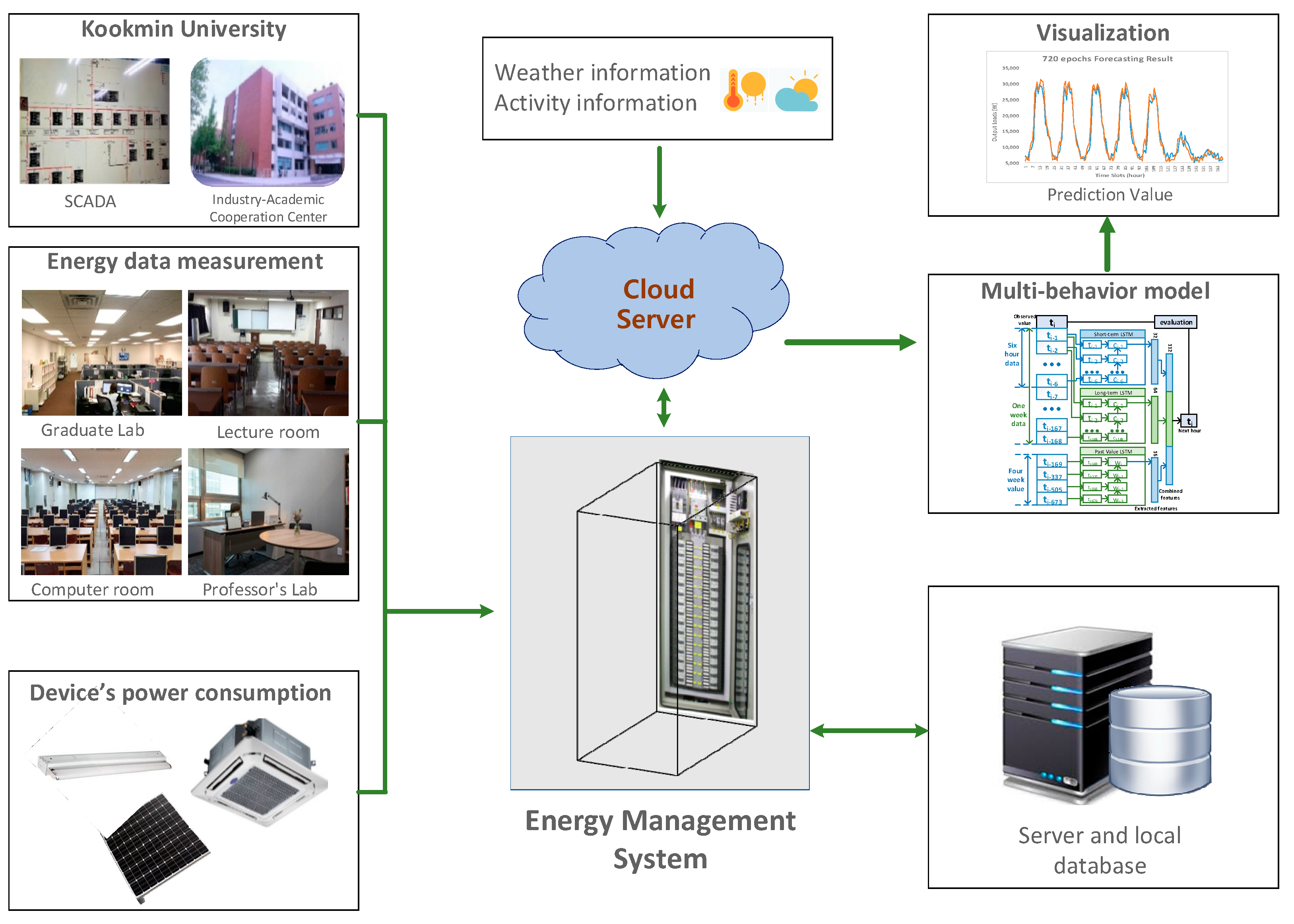
Figure 1 shows the overall architecture of the proposed building energy management system at Kookmin University. The RETIGRID energy management system collects statistical information from the building’s power system and sends it to the server. The data include energy measurements from labs, lecture rooms, computer rooms, and personal offices. They also include power consumption data for standard equipment, such as air conditioners, projectors, and light bulbs. The data are stored in a secure local database for further processing. Additional information about weather and daily activities is added to the data before prediction. A novel neural network is responsible for predicting the output load value; its output is presented to users in the form of graphical visualization. Based on the characteristic of the STLF and specific input data of Kookmin University, we propose a unique scheme and a new LSTM-based model for STLF. The main contributions of this paper are as follows:

• We briefly review the characteristics of STLF and the requirements for an accurate AI model for Kookmin University’s output load data. A unique scheme for STLF for building energy management systems is proposed.
• The main contribution in this work is the multi-behavior with bottleneck features LSTM model for use in STLF. This novel model provides more accurate and stable approaches to STLF and is applied to Kookmin University’s output load data.
• To investigate the efficiency of the proposed model, we build and analyze several models and metrics for evaluation. The corresponding experiments, data preparation, and model training are presented in detail.

The remainder of this paper is organized as follows. Section 2 describes related works, includes a novel approach in STLF and the requirement of a novel bottleneck features LSTM model for better accuracy. Section 3 provides the working scheme and the proposed model, including the overall architecture and practical development. Section 4 discusses the load data characteristics and their application. Section 5 details the proposed model and its results. The proposed model is compared with traditional machine learning and neural network approaches, including the k-nearest neighbor (KNN), convolutional neural network (CNN), and single-model LSTM. Section 6 summarizes the conclusions and suggestions for future research.

2. Related Works

STLF plays an important role in modern energy management systems, and it has been widely studied based on approaches such as traditional forecasting, machine learning, and deep learning models. Traditional forecasting has been thoroughly investigated and widely applied because of its high computational speed, robustness, and ease of implementation [10]. Machine learning methods and their expansions have been the subject of research interest for several decades; they include linear regression [11,12], multiple linear regression [13,14], and KNN [15]. For applications based on linear forecasting, these models are an excellent choice as they reflect the relationships among the features of output load and relevant factors. In these methods, the KNN approach is widely used in load forecasting due to a fast calculation time, high accuracy, and flexibility with different types of data. Therefore, we consider KNN in this study as a comparison method to highlight the performance of the LSTM model. The disadvantages of machine learning methods are prone to issues related to linear problems, which restrict the use of linear regression methods, particularly for nonlinear models. Other methods, such as support vector regression [16] and the decision tree [17] can work with non-linear problems. However, they cannot adapt to time series data and they cannot remember previous features in the long term.

Various ANN-based techniques have been introduced to overcome the challenges of nonlinearity and complex relationships in load data. The general ANN techniques include feedforward neural networks (FFNN) and backpropagation neural networks [18]. Compared to other machine learning methods, FFNN is more suitable for load forecasting due to its ability to work with nonlinearity and complex data. However, the FFNN is not effective in time series data analysis. Taking advantage of neural networks, deep learning has been introduced as a powerful tool for data analysis and prediction in many fields of research. Deep learning is based on the same concept as that of ANN as it uses a neural network to learn and adapt to unique situations. Nonetheless, the capability of ANNs is boosted in deep learning by raising the number of layers and taking advantage of their structure [19]. Thus far, deep learning has demonstrated an essential role in many areas, and it has become more popular than methods such as face recognition and automatic tracking. CNNs and RNNs are most widely applied in image processing and data analysis [20]. With these advantages, CNNs and RNNs can work with time series data and are also useful in STLF [21].

LSTM [22] is developed based on the RNN structure. It is fine-tuned to cope with the problems of time series data, including delays and relatively long intervals between forecasting and handling of important events [23]. Apart from LSTM, many methods can be used to address the gradient issues of the RNN structure. Nevertheless, LSTM is useful in improving long-term memory and ultimately achieving superior performance in STLF [24,25]. Therefore, RNNs and LSTM have proven to be beneficial and are widely used in STLF for building energy management systems [26,27]. However, the RNN and LSTM approaches have limitations with regard to the vanishing gradient and low accuracy with UUITFs [8,9]. LSTM in STLF can also lead to the loss of necessary data during the training process and is unsuitable for parallel computing. Concretely, it cannot process the task of computing wasteful usage and the time consumption of resource management. Given the strict requirements of building load forecasting, previous models have not been significantly effective. Hence, establishing a new appropriate model with a high accuracy and adapts to the UUITFs is required for the STLF.

3. Multi-Behavior with Bottleneck Features LSTM Model for Short-Term Load Forecasting

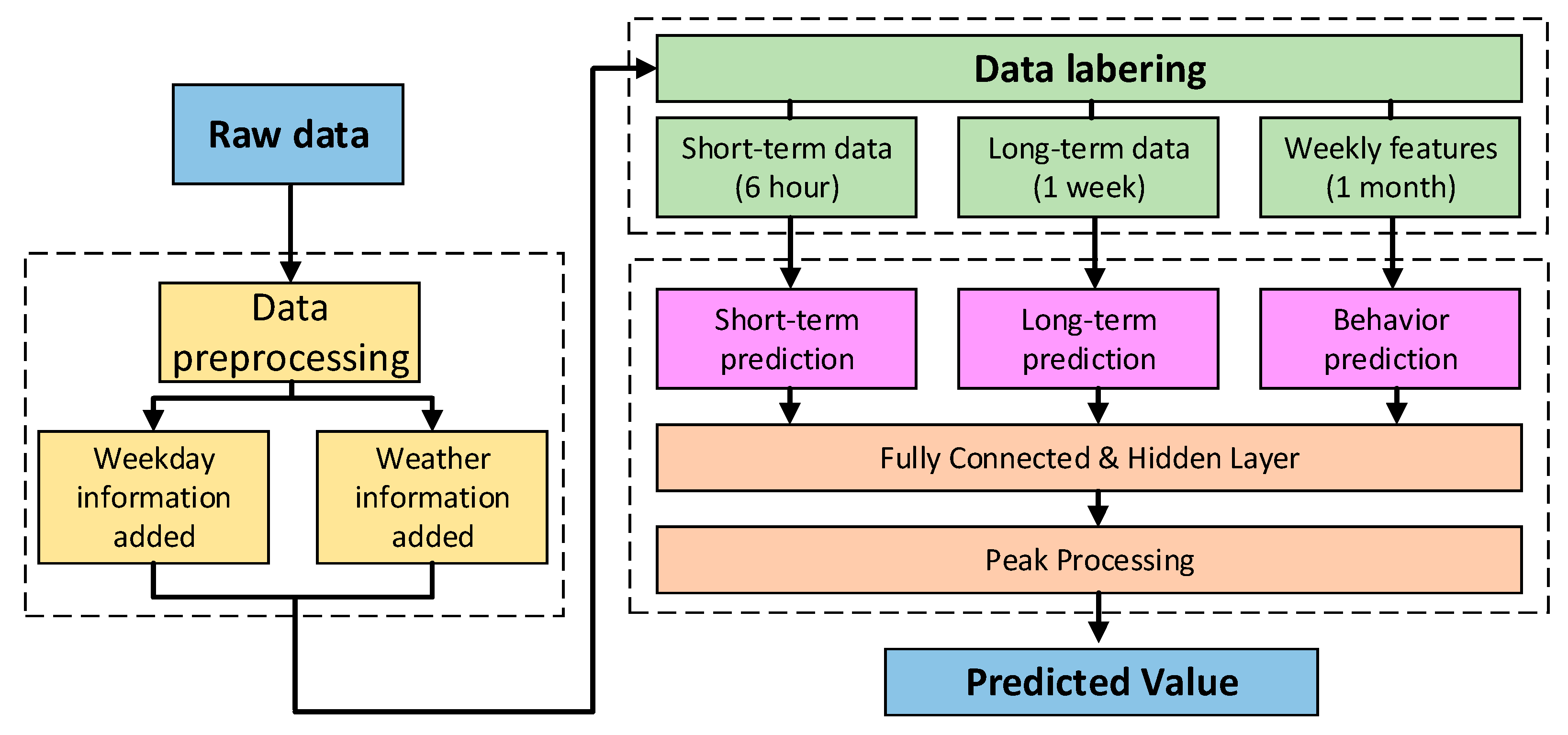
Figure 2 shows the overall architecture of an STLF scheme for a building energy management system. Raw data are collected for the preprocessing phase, during which the system “cleans” the signal to remove any unwanted components or features from the variables to be modeled. In our scheme, we do not remove outliers as they reflect the variations in activities across an entire building and are therefore necessary for model operation.

In support of pattern recognition, the raw data are augmented with additional data, including weekday and weather information, to account for the impact of fixed weekly schedules and weather on energy consumption. The data are then collected and divided into three categories per sample: short-term data (6 h), long-term data (1 week), and previous information (4 weeks). Each sample is labeled and fed into the multi-behavior with bottleneck features LSTM model to generate the final forecasting value.

3.1. LSTM Method for Different Time Scales

Based on time intervals and applications, load forecasting can be divided into several categories, including short-term, mid-term, and long-term intervals [28]. In this section, we introduce and analyze our approach to short-term forecasting using an LSTM network to increase the overall accuracy of traditional LSTM-based models. Based on the characteristics of short-term forecasting and LSTM-based models, the proposed LSTM model for different time scales is introduced to overcome the disadvantages of traditional methods.

3.1.1. Recurrent Neural Network (RNN)

The RNN is a special type of ANN. In the RNN, the output of one unit is fed into another unit to create a network with an internal state (memory) and temporal dynamic behaviors. With their unique structure, RNNs can analyze a sequence of data with dynamic behaviors between nodes. RNNs are widely used in series pattern recognition applications, including handwriting recognition [29], speech recognition [30,31], and time series data prediction.

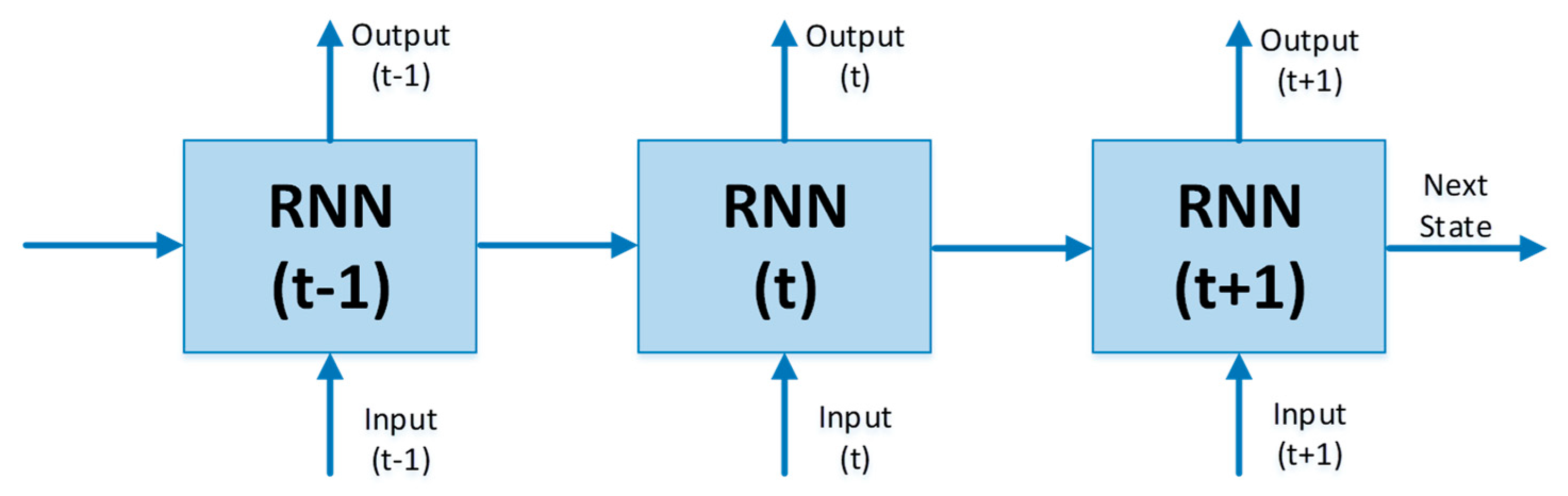
RNN nodes are connected in a sequence; that is, one node in a layer is fed to other nodes in the next layer (Figure 3). Each node in the RNN has its activation function and each connection has a temporal weight. A node can be an input, an output, or a hidden node. RNNs are typically used in supervised learning, in which each input is “labeled,” i.e., the output target is assigned according to the individual input. At a specific time step, the RNN cells calculate the output by using their activation functions and weight matrix. Using the input data and output of the previous RNN, the current RNN can combine the input and internal state of the network. The sequence error is calculated as the sum of the deviations of all outputs generated by the network. In the case of multiple sequences, the error is the combination of each sequence.

3.1.2. Long Short-Term Memory (LSTM)

LSTM is an improvement of the RNN architecture [32] used in time series data convergence. A typical LSTM cell has a fixed structure that comprises an input gate, an output gate, and a forget gate. In particular, the LSTM cell is used to store weight in the long term and its gates allow the memory to move in and out during the training and testing phases. By taking advantage of its ability to access long-time intervals at different events in a time series, LSTM works well for time series data processing. It is also suitable for exploding and vanishing gradient problems that occur in training traditional RNNs.

A typical LSTM architecture comprises a dynamic structure of units containing three gates to control the input information and memory as they go through the LSTM units (Figure 4). These units are responsible for extracting the features and dependencies of the input sequences. In an LSTM unit, the gates control the values flowing into the cell and the way the input pattern is “memorized.” The weights of the connections between gates determine how the gates operate.

The forget gate layer decides what information is forgotten. This gate obtains input data from h_t−1 and x_t, combined with the sigmoid active function: with an output value close to 1, the gate can carry almost all information; when the value is close to 0, the gate removes all previous information.

$$f_t = \sigma (W_f·\left[h_{t-1},x_t\right] + b_f)$$

(1)

The information subsequently passes through the input gate layer, where it is stored by the cell state; the weight for the next state is then updated. In this phase, the sigmoid layer decides which value to update, and a tanh activation function creates a vector of new values C_t that can be added to the state. The state is updated by combining the outputs of these functions.

$$i_t = \sigma (W_i·\left[h_{t-1},x_t\right] + b_i)$$

(2)

$${\tilde{C}}_t = \tanh (W_C·\left[h_{t-1},x_t\right] + b_C)$$

(3)

In the next phase, the cell state is updated based on the previous output value. The old state is multiplied with f_t to forget the information fed into the forget gate. The new candidate value C_t is subsequently added and scaled according to the degree to which each state value should be updated.

$$C_t = f_t\ast C_{t-1}\ast {\tilde{C}}_t$$

(4)

In the final step, the cell decides the output values based on the cell state. First, the sigmoid layer decides which part of the cell state is the output. Second, the cell state passes through a tanh function (with values between −1 and 1) and is multiplied with the output of the sigmoid gate.

$$o_t = \sigma (W_o·\left[h_{t-1},x_t\right] + b_o)$$

(5)

$$h_t = o_t\ast \tanh (C_t)$$

(6)

LSTM networks are fine-tuned to cope with the exploding and vanishing gradients that may occur in traditional RNNs. LSTM networks are also effective in classifying, processing, and making predictions based on time series data. The advantage of LSTM over RNNs, hidden Markov models, and other sequence learning methods in various applications is its high insensitivity to gaps in length.

3.1.3. LSTM-Based Model for Input Data of Different Time Scales

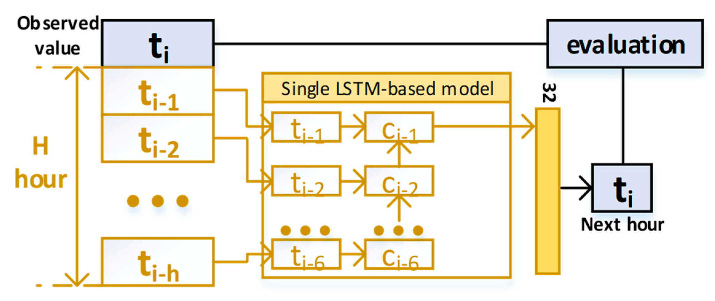
Relative to other ANN models, such as MLP or CNN, LSTM can process long-term input data and reflect time series data characteristics because of its unique structure and the recursive connections between nodes. The proposed LSTM approach of different time scales is expected to improve forecasting models’ capability to reflect short-term activities, including UUITFs, and long-term time series input data characteristics, which are a significant research topic at present. To highlight the ability of the proposed approach of different time scales and the improvement in the forecasting model, a single LSTM-based model is considered as a baseline for comparison. The fundamental concept of the proposed approach is the unique combination of the features of LSTM networks with long- and short-term input data, including the ability of the latter in terms of dealing with UUITFs with intrinsic weighting and the forecasting ability of the former. When the input data fed to the model lengthen, the importance of recent data in weight training is decreased and the information is lost. In this case, the training of the forecasting model cannot progress further, and the forecasting performance decreases. A possible solution is to use input data with a short duration, such as 6 h (Figure 5). Through this approach, the importance of recent data in the training phase increases and the data become suitable for STLF. However, the model’s capability of analyzing long-term patterns is greatly weakened thus reducing the overall prediction accuracy. From this point, the LSTM model for short-term input data will be referred to as the short-term single-model LSTM, and that for long-term input data will be referred to as the long-term LSTM-based single model.

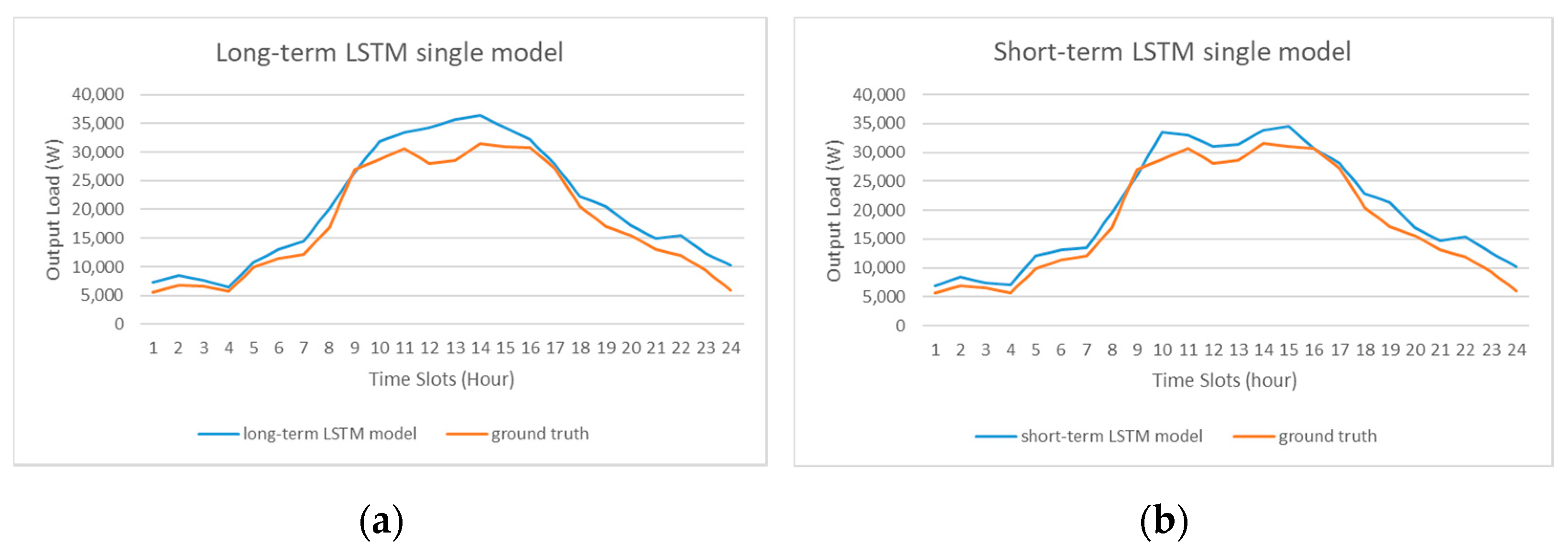
The ability of a forecasting model to adapt to UUITFs and maintain output values close to the ground truth is essential. If a model can track UUITFs and adapt quickly, it can be considered robust in terms of UUITF prediction. The relation of reactivity and accuracy throughout the proposed model is presented with the forecasting results of many unexpected events that decrease the ground truth value and significantly affect the accuracy of the model.

In Figure 6, a temporal variation due to UUITF can be observed in the orange line (ground truth) between time slots 11 and 14. The long-term LSTM in (a) does not reflect the UUITF, whereas the short-term LSTM in (b) can track the UUITF as it approaches the ground truth. However, the short-term LSTM is not robust in terms of forecasting accuracy as indicated by the difference between the blue line and the ground truth from time slots 18 to time slot 24; the same is similar for the UUITF (b). Thus, in order to maintain the prediction accuracy of the proposed model, the input data must be kept for a long duration and the information about recent events must be preserved.

Given the limitations of long-term LSTM and short-term LSTM, the requirements of combining their advantages should be met in load forecasting for building management systems. The multi-behavior with bottleneck features LSTM model was developed based on the approach of different time scales, and further adjustments are made to increase the stability of the forecasting process. In the next section, we introduce the multi-behavior with bottleneck features LSTM model to improve the accuracy and stability of STLF.

3.2. Multi-Behavior with Bottleneck Features LSTM Model for Short-Term Load Forecasting

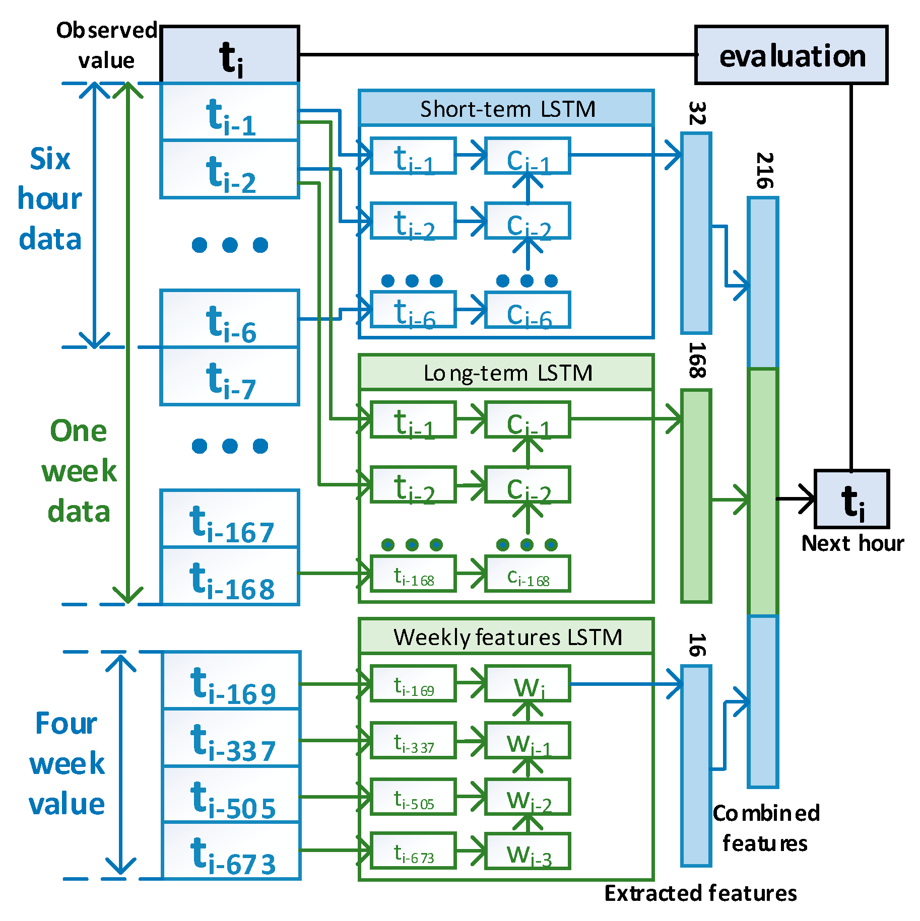
Figure 7 shows the overall architecture of the proposed framework, which incorporates multiple time scales and weekday information approaches. The input data of multiple time scales, including a 6 h duration and 1 week duration, are fed into the model, in which they are divided into short duration processing and long duration processing. The two networks are responsible for extracting the corresponding data features for the input data of each time behavior. Conversely, previous weekday information is analyzed to extract data for weekly features. Subsequently, the output is oriented to the fully connected layer, which can combine the information from three different networks to determine the load forecast for the next hour. The overall architecture of the multi-behavior with bottleneck features LSTM model is inhered from previous studies [8,9].

The model can maintain the overall forecasting accuracy of a baseline LSTM/RNN model, reflect the recent data characteristics to predict UUITFs, and emphasize the importance of weekly features in load forecasting. Finally, a multi-behavior with bottleneck features LSTM framework, which combines the bottleneck features of short-term, long-term, and weekly feature LSTM networks, is proposed to exploit the combination of a short-term LSTM that can re-emphasize UUITFs, the forecasting ability of long-term LSTM, and the features from previous weekday data.

The combination of the aforementioned features requires a neural merge layer. The input features exhibit different characteristics, leading to reduced overall accuracy. In this model, each feature provides a different approach that can work on its own. Thus, a single fully connected neural network is not suitable for combining output values. Fortunately, we can use a neural network with bottleneck features to establish a connection between features as the outputs of the hidden layer can be used as inputs for the other layers. Each neuron in the extracted feature layer receives one input from the previous LSTM layer, and it is calculated as

$$z_i=x_{LSTM}·w_i+b_i$$

(7)

where x_LSTM is the output of the previous LSTM layer, w_i is the weight of the neural node, and b_i is the bias. The activation function is subsequently calculated as:

$$f(z_i)=\{\begin{array}{l}0.01z_i\hspace{1em}for z_i<0\\ z_i\hspace{1em}for z_i\ge 0\end{array}$$

(8)

Through bottleneck features, the disadvantageous application of multiple time behaviors turns into the use of a high number of classes in the next layer. The short-term LSTM-based approach emphasizes a relationship with recent data by weighting such data according to trained weights. By contrast, the long-term LSTM-based model can analyze long-term patterns, such as periodicity. The weekly feature LSTM-based model performs relatively well because of the stable schedule of the university. Therefore, the proposed multi-behavior with bottleneck features LSTM framework can provide reactivity and accuracy by considering the two concatenated embedded results.

To investigate the efficiency of the proposed model, we analyzed several other models and the metrics for evaluation. The compared models were the short-term single-model LSTM, long-term single-model LSTM, feedforward neural network (FFNN), two-dimensional convolution neural network (2D-CNN), and KNN. The performance evaluation metrics included the root mean square error (RMSE), mean absolute error (MAE), coefficient of variation of the root mean square error (CV-RMSE), and mean absolute percentage error (MAPE). The corresponding experiments are presented herein, along with detailed information about data preparation and model training.

4. Data Analysis

4.1. Input Load Data

Data were collected from one building at Kookmin University, Seoul, Korea, by using the RETIGRID power monitoring system, which can manage the working data of a specific building. The energy management system collects the energy data of the building by using a smart meter that is specifically designed for the task. The data collected include the active power of the system and other parameters, such as reactive power, apparent power, phase current, phase voltage, power factor, and frequency. Data were collected over a period of 9 months, from 25 March 2019 to 18 December 2019, with 5 min intervals. High-quality detailed data suitable for analysis and prediction were collected at short intervals over a long period. Another advantage of this dataset is its stability because the university operates according to a fixed schedule for the duration of each semester. This fixed schedule is the main factor affecting the active load of the building as it plays an important role in total power consumption and stable power usage patterns. Along with important parameters affecting power consumption, we also tracked other useful parameters, such as temperature and hours of daylight, which contain information about regular activities and thus affect the total output load.

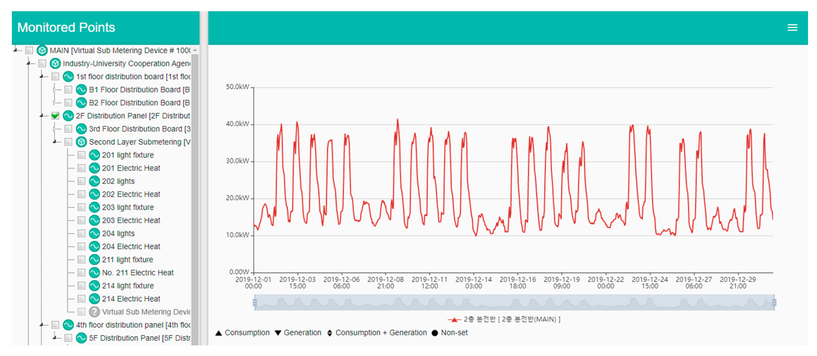
Figure 8 shows an example from the RETIGRID system that displays the active load of the building for one month (December) along with general study activities. The first consideration is the minimum active load value, which occurs at the end of the day, usually between the cessation of activities at 9 p.m. until the start of a new working day at 8 a.m. the following morning. We can assume that this power consumption is necessary to maintain critical equipment and machines in the building, such as heaters, ventilation, light bulbs, or computer servers. The second consideration is the active load that is significantly affected by work activities. Power consumption drops off significantly during the weekend, and the active load on Sunday is lower than that on Saturday mainly because of the lack of classes and study activities. These characteristics were analyzed and considered to be representative of regular activities within other facilities and offices as a primary factor in further study and model design.

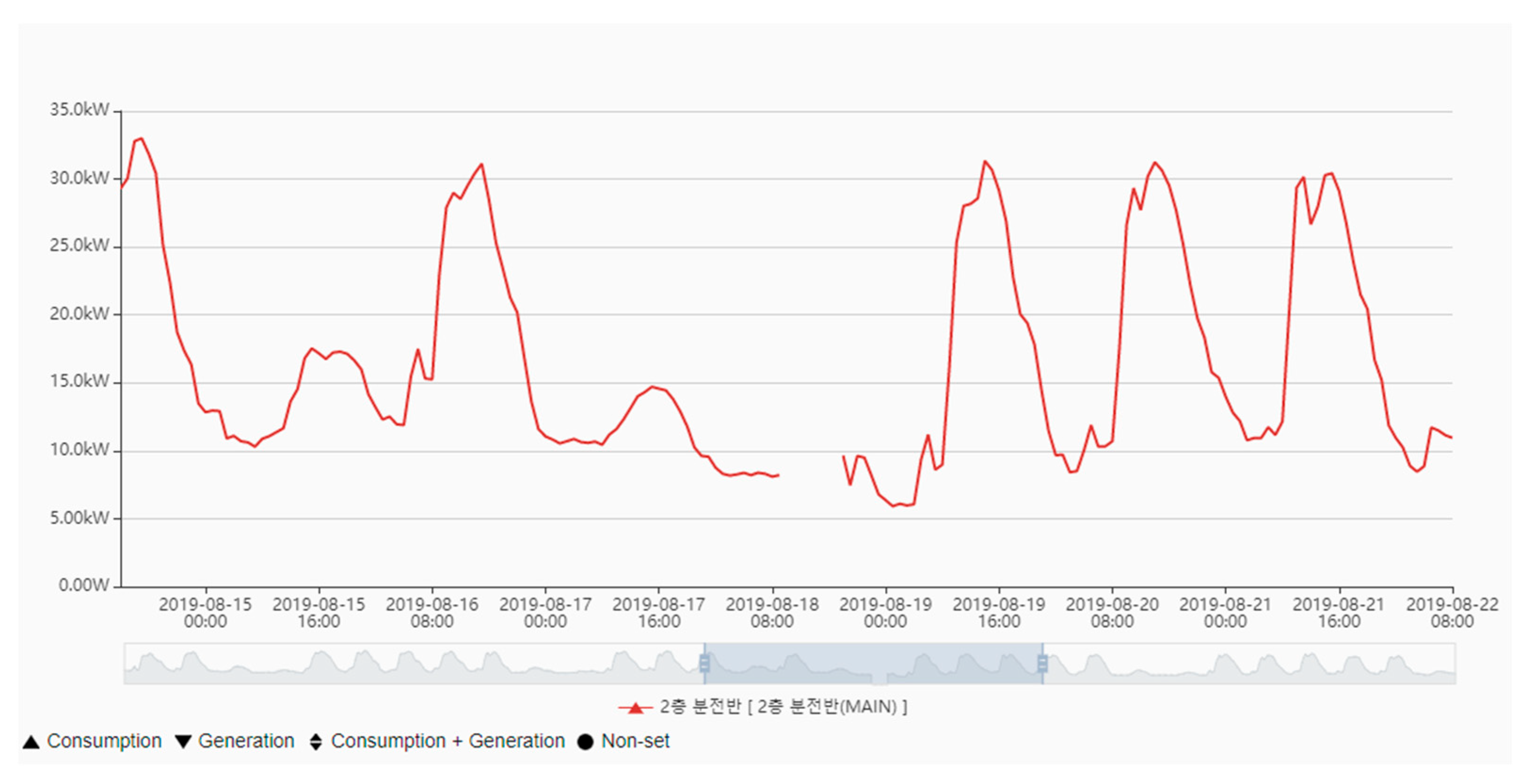
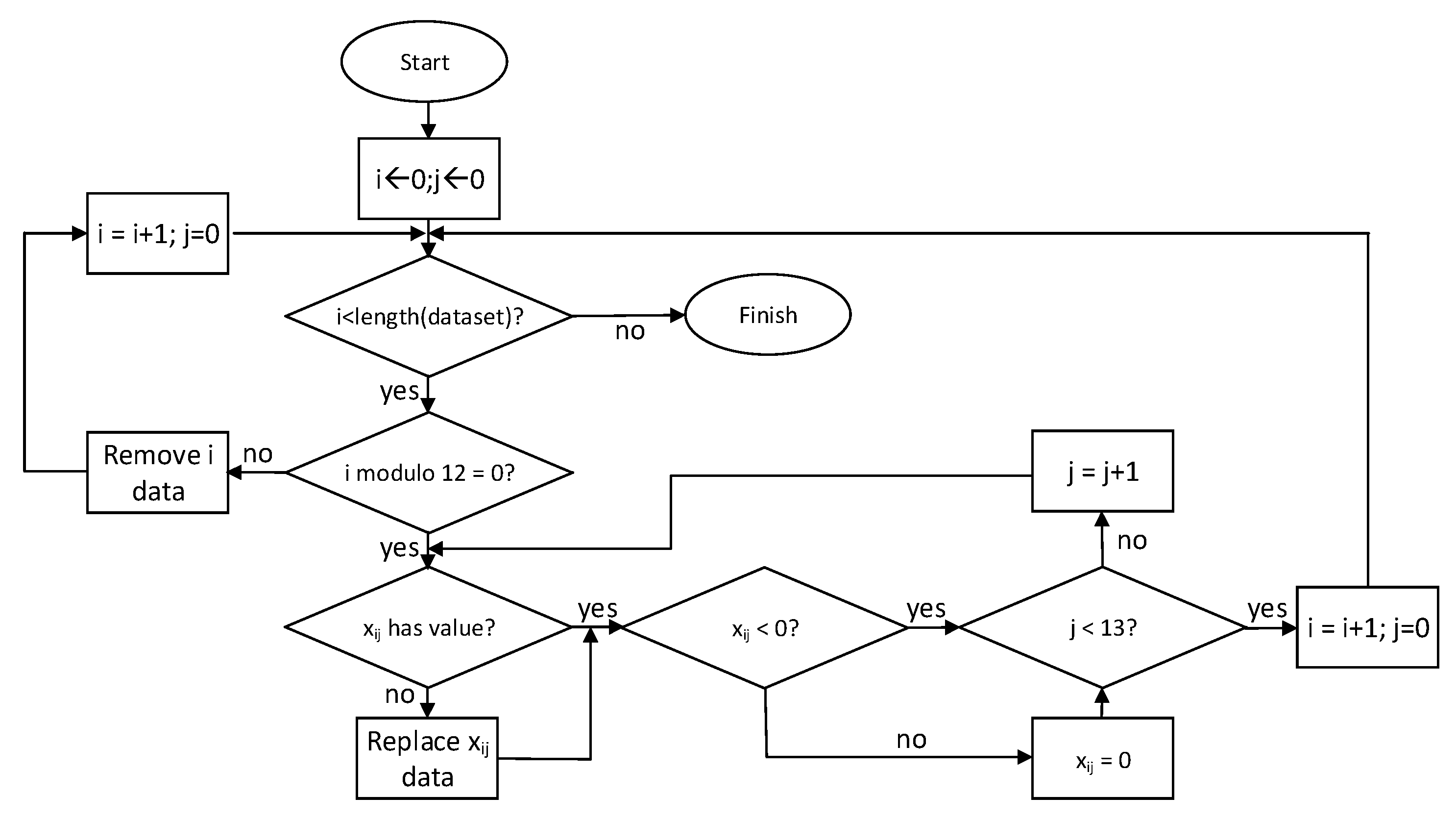
The load data had many disadvantages, including the lack of comparative data, such as those from other buildings. The system also had minor errors resulting in the loss of data for short periods that had to be filled or replaced. Figure 9 shows an example of missing data for a short period from 10:00 a.m. to 16:00 p.m. on 19 August 2019. However, the number of errors was small, and they did not affect the overall result of the data analysis and prediction. The overall flow of the data preprocessing phase is shown in Figure 10.

4.2. Preprocessing

The raw data collected by the energy management system included the system’s active power, reactive power, apparent power, current phase, voltage phase, power factor, and frequency. Other data, such as temperature and hours of daylight, were collected separately and combined to provide information on daily activities. Based on the previous data analysis, weekday information was added to the input data. Holiday dates were also collected and combined with the input data because they also affect daily activities. As missing data were checked and filled, we accepted the small errors caused by gaps in the data in cases when the missing values could not be obtained. Another problem we needed to consider was that the sampling frequency for the load data, which were collected every 5 min, was too high and did not provide sufficient stability for the current study. The short time interval between data points caused instability in the data analysis and a high level of noise. To address this issue, we increased the time interval to 1 h by using the accumulated partial load values. The preprocessing in the building energy management system is shown in Figure 10.

During the preprocessing stage, we divided the input data into a training set of 9 months and a test set of 3 months. The duration of the input sample was optimized to provide sufficient information for prediction while maintaining a reasonable operating speed. The input data can therefore be considered as a composition of data samples from time step t − d to t − 1 and can be used to predict load power at step t. Relative to previous STLF problems, the input data from the university were stable and contained enough relevant information to obtain a reasonable prediction. The data were divided into one-week batches (24 × 7 h) with no negative impact on the training process. With this method, the batches were fed continuously into the model and the temporal variations could be reflected in the time series data.

The input data included short-term (6 h), long-term (1 week or 168 h), and weekday information for 1 month (4 samples). These samples were collected and labeled before being fed to the model. Each sample also included the real value of the power load for the next hour as the output value for model training. The data labeling process is the most critical part of our scheme as it involves the construction of the complete input dataset to be fed to the LSTM-based model.

4.3. Weekday Information and Input Data Improvement

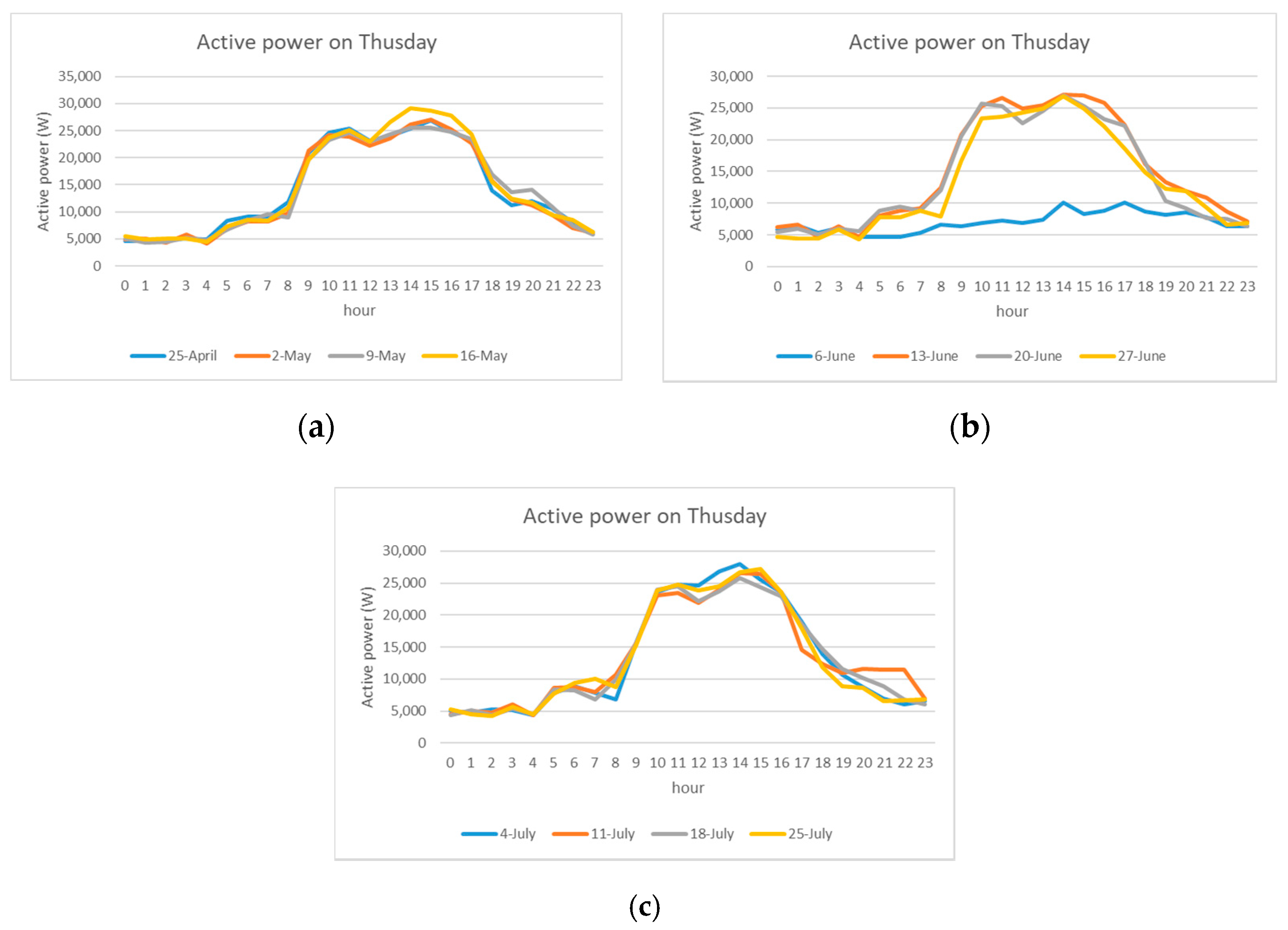
The total power consumption of one building is affected by the daily activities of the people, machines, and facilities within it. This characteristic is significant in schools and public facilities, where the number of machines and devices is constant and daily routines are the primary variable affecting the output load. Figure 11 shows the active power on all Thursdays of the months of May, June, and July. The active power levels for all hours in May were almost the same (a), thus indicating the consistency in power consumption characteristics depending on the university’s schedule. Similarly, the active power levels in July (c) were consistent across all weeks. However, the peak active power for July was higher than that for May because high temperatures at this time led to increased power consumption by air conditioning equipment. As for June (b), 6 June was exceptional because its active power was much lower than those of the other days. As 6 June is a national holiday in Korea (Liberation of the Fatherland Day), all daily activities in the building ceased. This characteristic can be used to increase the accuracy of the forecasting model.

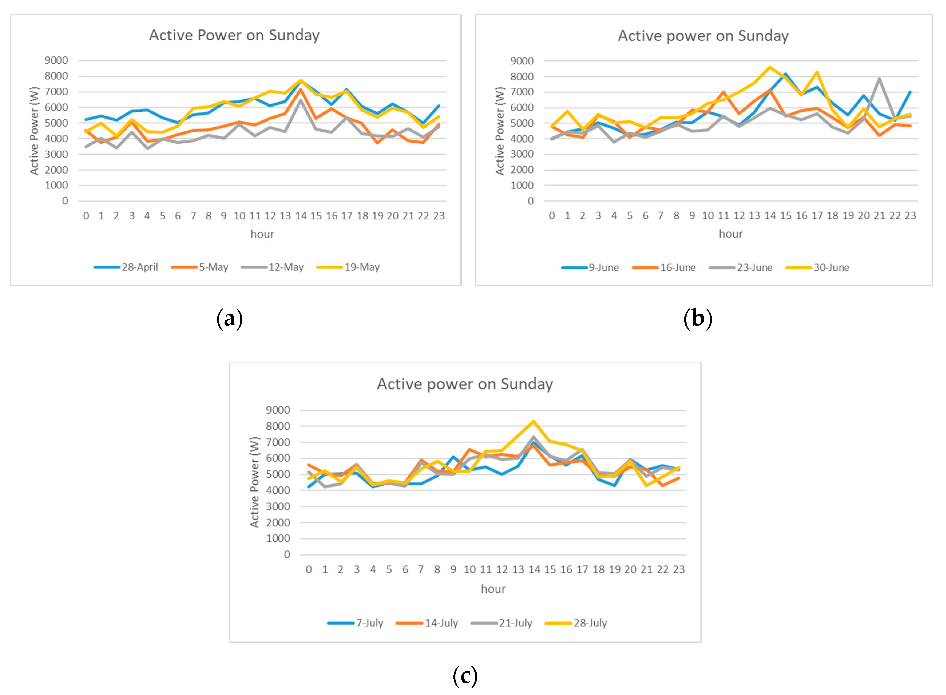
Daily routines are reflected in data for weekends and holidays, during which activities cease and supporting devices stop running, leading to shallow power consumption and different patterns relative to those for typical weekdays. Figure 12 shows the active power for a Sunday when most activities were halted, except for those of a small number of people conducting personal business. Active power levels were collected for May (a), June (b), and July (c) under the same conditions as those in Figure 11. The data proved to be difficult to predict because of the lack of any recognizable pattern. As the conditions on holidays differ from those on regular weekdays, including the information from these periods should improve model accuracy. Therefore, the data on daily routines and weekly features for a given weekday are critical in output load prediction. Weekly features reflect a regular working routine and stable schedule and were thus applied to the LSTM network to collect information and predict the output load.

5. Implementation and Experiments

5.1. Forecasting Model Implementation

The multi-behavior with bottleneck features LSTM architecture has 64 hidden LSTM units and 64-dimension bottleneck features. The input of the short-term LSTM-based model was set to 6 h and that of the long-term LSTM-based model was set to 24 × 7 h (one week). The bottleneck features of the multi-behavior LSTM-based model were concatenated with 32, 64, and 16 ratios and fed from the short-term, long-term, and weekly feature LSTM-based models, respectively. The weights of all LSTM cells were initialized according to the work of Xavier [33], and DROP was applied [34] with 0.7 keeping probability. Leaky ReLU [35] was used as the activation function for the hidden and output layers of the combined features; its formula is defined as

$$f(x) = \{\begin{array}{l}0.01x\hspace{1em}for x<0\\ x\hspace{1em}for x\ge 0\end{array}$$

(9)

The loss function applied to the training phase was MSE. We selected the stochastic gradient descent (SGD) as the iterative optimization algorithm. The models were trained with a minibatch size of 168 by using the ADAM solver [36], and the learning rate was 0.0005. The proposed multi-behavior with bottleneck features LSTM model was trained over 1000 epochs.

5.2. Data Preprocessing

The input data were split into a training set of 9 months and a test set of 3 months. The training data can therefore be considered as a dataset from time step t − d to t − 1 and can be used to predict load power at step t. The data were divided into one-week batches (24 × 7 h) with no negative impact on the training process. All the values of each field were normalized to [−1; 1]. A single batch was combined with the continuous 168 composed data, each of which consisted of continuous duration. The entire batch group was shuffled and 70% of an arbitrarily selected batch group from the total number of batches was used for the training data; the remaining batch group was used as the test data. In this regard, the continuity of the sample data in each batch was maintained to help determine whether the model can reflect temporal variation in load forecasting.

5.3. Performance Evaluation Metrics

The following error evaluation metrics were used to evaluate the overall results of the load forecasting scheme.

Root mean square error (RMSE) measures the difference between forecast values and observed values. The RMSE represents the square root of the differences between forecast values and observed values; that is,

$$RMSE= \sqrt{\frac{1}{N}{\displaystyle \sum _{i=1}^N{(P_f-P_o)}^2}}$$

(10)

where N is the number of observations, P_f is the forecast value, and P_o is the actual value.

Mean Absolute Error (MAE) is the average of absolute errors. It can effectively reflect the accuracy of the forecasting value error and is defined as

$$MAE= \frac{{\displaystyle {\sum }_{i=1}^N}|P_f-P_o|}{N}$$

(11)

The coefficient of variation of the root mean square error (CV-RMSE) can compare datasets or models with different scales. The CV-RMSE is also known as the normalized root mean square error (NRMSE) and is calculated as

$$NRMSE= \frac{1}{y_{\max }-y_{\min }} \sqrt{\frac{1}{N}{\displaystyle \sum _{i=1}^N{(P_f - P_o)}^2}} = \frac{RMSE}{\overline{y}}$$

(12)

The mean absolute percentage error (MAPE) is a performance matrix in statistics that can be used as the loss function for forecasting problems. It is usually expressed as a ratio defined by the following formula:

$$MAPE= \frac{1}{N} {\displaystyle \sum _{i=1}^N\left|\frac{A_t - F_t}{A_t}\right|}$$

(13)

We selected RMSE and MAE to evaluate our proposed scheme as they are suitable for evaluating short-term predictions, such as hourly load forecasting. The NRMSE and MAPE are more popular than other data of different scales.

5.4. Experimental Setup and Evaluation

5.4.1. Experiments with CNN, FFNN, and KNN Regression Models

The experimental setup used Python version 3.7.4 [37] and TensorFlow version r1.14 [38]. To compare the performance of the proposed model with that of other machine learning models, we need to apply different learning algorithms to the output load dataset. In this study, we considered FFNN, KNN, and 2D-CNN models for the LSTM comparison. These models were chosen since they are widely used in STLF along with the LSTM mode [21,25]. In [25], the LSTM method was compared with an FFNN and KNN model. The MAPE of the LSTM scores outperformed those of the FFNN and KNN, thus demonstrating the effectiveness of LSTM in load prediction. Based on this study, we selected the FFNN and KNN models as comparison candidates in STLF using the dataset. For further comparisons, we also tested the dataset with the 2D-CNN model. The experiment was conducted using the output load input data without weekday and holiday information.

Table 1. Performance of the FFNN, 2D-CNN, and KNN.

	FFNN (961 Epochs)	2D-CNN (923 Epochs)	KNN
RMSE	3407	2759	6260
MAE	2493	1939	3777
NRMSE	13.12	10.15	24.04
MAPE	28.19	27.71	60.31

shows the performance scores of the FFNN, CNN, and KNN models for the output load dataset. The FFNN model used herein had a typical architecture with three hidden layers and one output node. The duration input data were set to 1 day (24 h). We used two different hidden layers with a size of 168 for the prediction model. The activation function for the combined feature layer was ReLU and the loss function was MSE. We selected the SGD as the iterative optimization algorithm by using the ADAM solver. The proposed multi-behavior with bottleneck features LSTM model was trained over 1000 epochs. For the CNN model, we only used two convolutional layers with a ReLU activation function. Similar to that done for the FFNN, we selected the SGD, ADAM solver, and training over 1000 epochs for the CNN model. The KNN was easy to implement and was thus used herein for regression with three neighbor functions. As the most straightforward technique, the regression KNN did not have a high accuracy, with its RMSE score being 6260 and its MAE score being 3777. The 2D-CNN had the best performance scores with an RMSE of 2759 and MAE of 1939. The FFNN’s performance scores were relatively poor, with its RMSE being 3407 and its MAE being 2493.

5.4.2. Single LSTM Model

The single LSTM-based network only includes a single bottleneck feature LSTM-based network connects with a fully connected layer. Experiments were performed with two different single LSTM-based network models: a short-term input data model (6 h duration) and a long-term input data model (1 week duration). Two different test sets were used: one included only the raw data, and the other included the raw data plus weekday and holiday information. We also investigated whether the LSTM network was a robust model for load forecasting and residential energy management systems relative to other machine learning methods. First, we compared the performance of the long-term and short-term single-model LSTM networks with those of previous machine learning techniques and then with that of the proposed model. For the training process, we ran with a large number of epochs and chose the best results from them. Therefore, we can consider if the model has overfitting problems or not.

Table 2. (a) Performance of long-term and short-term single LSTM models using a dataset without weekday and holiday information. (b) Performance of long-term and short-term single LSTM models using a dataset with weekday and holiday information.

(a)
	Short-Term Single LSTM Model (430 Epochs)	Long-Term Single LSTM Model (310 Epochs)
RMSE	2118	1778
MAE	1522	1370
NRMSE	8.07	6.77
MAPE	19.36	19.82
(b)
	Short-Term Single LSTM Model (550 Epochs)	Long-Term Single LSTM Model (460 Epochs)
RMSE	1891	1691
MAE	1423	1268
NRMSE	7.20	6.44
MAPE	21.65	20.83

a shows the overall performance of the short-term LSTM-based single model (6 h) and that of the long-term LSTM-based single model (1 week). The LSTM-based single model had better performance scores than the other machine learning methods in terms of RMSE, MAE, NRMSE, and MAPE. The RMSE of the short-term LSTM-based single model LSTM was 2118 with 430 epochs; this result was much smaller than those of the FFNN and 2D-CNN. The long-term LSTM-based single model is even better with an RMSE score of 1778 after 310 epochs. The MAE scores of the LSTM-based single model were also satisfactory at 1552 and 1370 after 1000 epochs. The NRMSE and MAPE scores, which are essential in scaled comparisons, were also high at 8.07 and 19.36 for the short-term LSTM-based single model and 6.77 and 19.82 for the long-term LSTM-based, respectively.

In the next step, we considered the improvement of the model’s performance with the addition of weekday and holiday information. The weekday and holiday information improved the performance of both short-term and long-term LSTM-based single models (Table 2b). This result was due to the improvement in schedule pattern detection, which mostly depended on weekday information. In this experiment, the long-term single network performed relatively well because it utilized additional information to predict the output value. Nevertheless, the short-term single LSTM-based model displayed robust performance in the detection of UUITFs. Figure 6 shows the ability of the short-term single-model to adapt to the UUITF relative to the long-term single-model LSTM.

5.4.3. Multi-Behavior with Bottleneck Features LSTM Network

The multi-behavior with bottleneck features LSTM network comprised three bottleneck LSTM networks connected to two fully connected layers: short-term LSTM (6 h), long-term LSTM (1 week), and weekday feature extraction (value from the same hour of the same weekday for the past four weeks). Experiments were performed with long- and short-term single-model LSTM networks and with all three LSTM networks. We used test sets with and without weekday and holiday information.

Table 3. Performance of the multi-behavior with bottleneck features LSTM model.

	Without Weekday and Holiday Information (860 Epochs)	With Weekday and Holiday Information (720 Epochs)
RMSE	1745	1518
MAE	1269	1146
NRMSE	6.42	5.59
MAPE	9.7	6.71

presents the load forecasting results obtained using the multi-behavior with bottleneck features LSTM network and the combined information from the long-term, short-term, and weekly feature LSTM subnetworks. Compared with the single-model LSTM network (Table 2), the multi-behavior LSTM-based model displayed better performance. With the weekday and holiday information, the RMSE scores decreased to 1518 after 720 epochs. The MAE also decreased to 1146 after 720 epochs. These results showed the multi-behavior with bottleneck features LSTM model to be more stable and accurate than the long-term single LSTM-based model, and that it outperformed other traditional machine learning methods, including CNN, FFNN, and KNN models. With the weekday and holiday information, the multi-behavior with bottleneck features LSTM model also had improved results, with its NRMSE and MAPE scores being 5.59 and 6.71 after 720 epochs, respectively.

To prove the capabilities of the multi-behavior with bottleneck features LSTM model in UUITF prediction, we should consider the prediction output relative to the real input data. Figure 13 shows the results for the multi-behavior with bottleneck features LSTM model with 720 epochs over one week. The short-term LSTM subnetwork enabled the model to keep track of the UUITFs while the long-term LSTM and weekly feature subnetworks maintained forecasting values close to the ground truth. The proposed model was robust when dealing with weekday forecasting because of the fixed schedule of work activities. However, its performance declined during the weekend when the schedule was not fixed and the pattern was difficult to recognize.

6. Conclusions

STLF is essential in energy management systems and energy market transactions, particularly for public facilities and offices. STLF plays an essential role in time series data analysis and building load prediction. The proposed scheme utilizes a multi-behavior with bottleneck features LSTM network and thus combines the advantages of different methods of time series data analysis to forecast output loads. Based on various experiments and implementations, we confirmed that the proposed model was robust in load forecasting using real-world test data from Kookmin University.

Compared with the single-model LSTM network, the proposed model displayed better performance with lower RMSE and MAE scores, and also the ability to adapt with the UUITFs in the building load forecasting. The proposed model also proved to be more stable and accurate than the long-term single LSTM-based model. Therefore, this study is a good reference for future research into different ways to achieve better solutions for STLF problems. With better performance, STLF can improve prediction accuracy and provide a significant amount of reliable information for management applications, such as reliability analysis, short-term switch evaluation, abnormal security detection, and spot price calculation.