DC-STGCN: Dual-Channel Based Graph Convolutional Networks for Network Traffic Forecasting

Abstract

Network traffic forecasting is essential for efficient network management and planning. Accurate long-term forecasting models are also essential for proactive control of upcoming congestion events. Due to the complex spatial-temporal dependencies between traffic flows, traditional time series forecasting models are often unable to fully extract the spatial-temporal characteristics between the traffic flows. To address this issue, we propose a novel dual-channel based graph convolutional network (DC-STGCN) model. The proposed model consists of two temporal components that characterize the daily and weekly correlation of the network traffic. Each of these two components contains a spatial-temporal characteristics extraction module consisting of a dual-channel graph convolutional network (DCGCN) and a gated recurrent unit (GRU). The DCGCN further consists of an adjacency feature extraction module (AGCN) and a correlation feature extraction module (PGCN) to capture the connectivity between nodes and the proximity correlation, respectively. The GRU further extracts the temporal characteristics of the traffic. The experimental results based on real network data sets show that the prediction accuracy of the DC-STGCN model overperforms the existing baseline and is capable of making long-term predictions.

1. Introduction

As the main communication means, the internet plays an important role in daily life, production and the military. The internet not only meets people’s daily communication needs but also contributes greatly to the development of the country. With the rapid development of data networks and the increasing demand for network traffic, wireless network operators need to guarantee the Quality of Service (QoS) of their networks, thus, leading to a need to plan their network traffic properly [1,2]. Traffic planning provides a scientific approach to allocate traffic, while network traffic forecasting provides a solution to the network traffic planning problem. Timely and accurate traffic forecasts are becoming increasingly important for network management and planning. Such forecasts enable managers to formulate resource allocation strategies in advance, and proactively manage upcoming overload events. Nevertheless, due to the complex temporal and spatial relationships between traffic flows, it is difficult for traditional forecasting models to accurately predict network traffic [3,4,5].

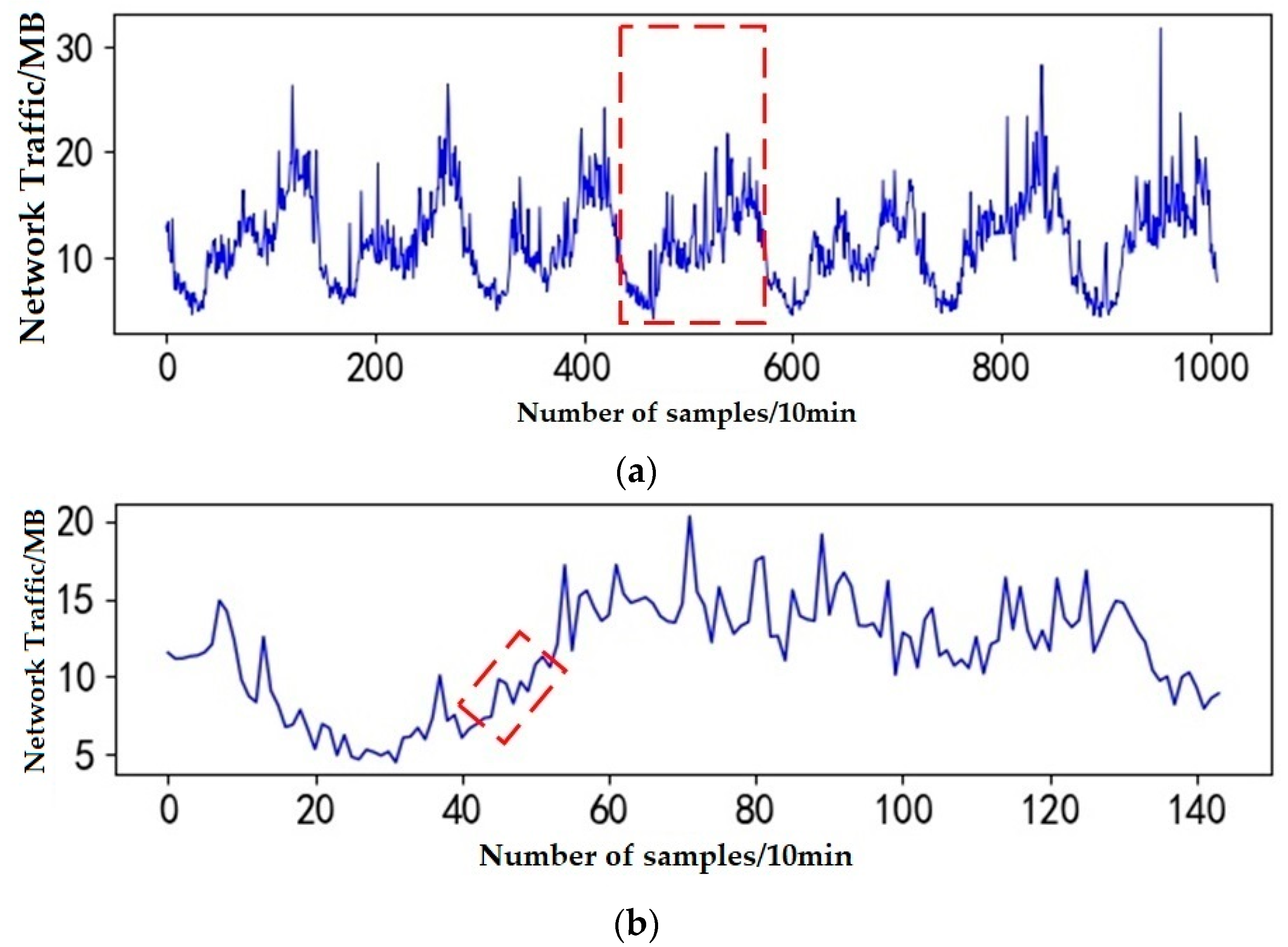
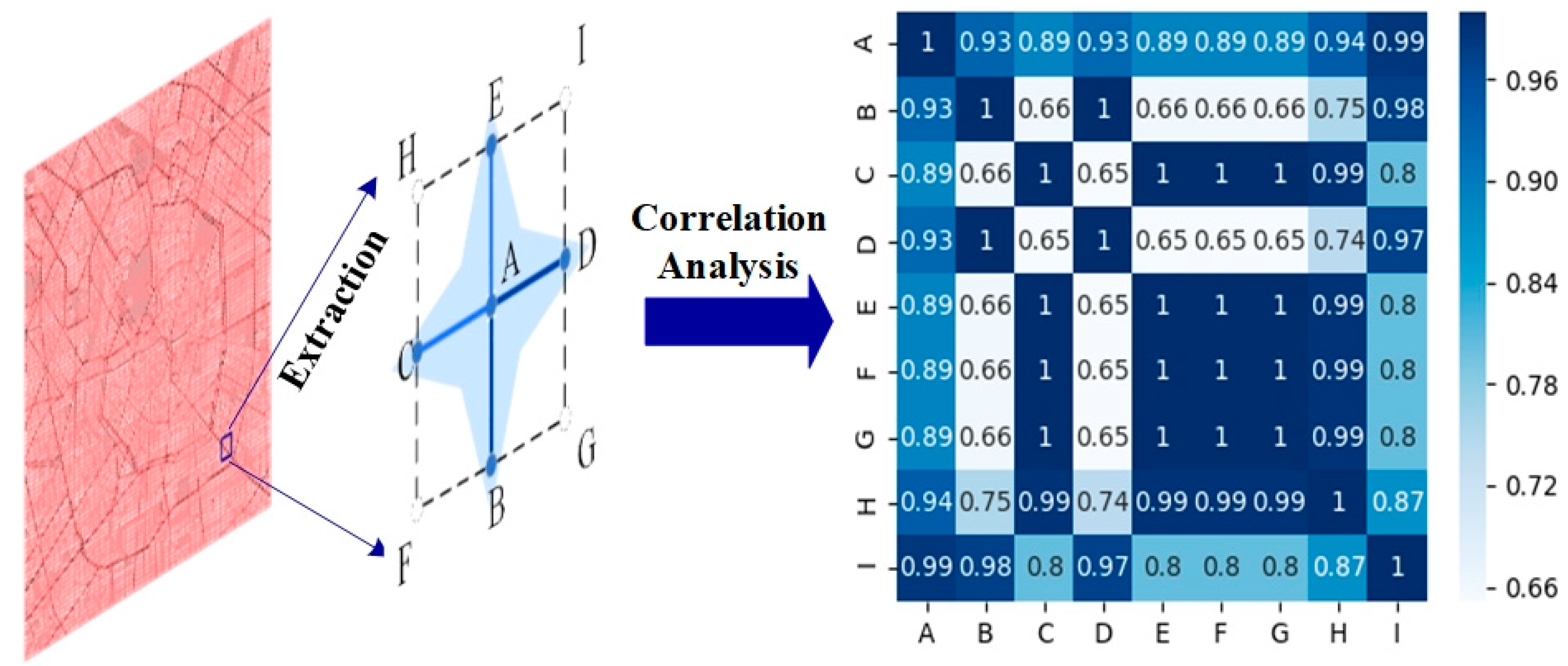
Network traffic prediction is a typical spatial-temporal sequence prediction problem, where the topology of the network nodes affects the traffic. The traffic data sampled between the nodes are not independent of each other. The spatial and temporal dependencies of network traffic are shown in Figure 1 and Figure 2. The line between each node in Figure 1 represents the weight of their interaction, where the darker the color the larger the weight value. It can be seen that for node A, its neighboring nodes in various locations differently affect this node while such effects are also time-dependent. The traffic variations at node A are shown in Figure 2a,b, over a week and a day, respectively. As shown, the network traffic is periodically changed over the week [6], and the traffic over the day also demonstrates high daytime and low nighttime variations. It is shown that the current network traffic is affected by the traffic at the previous times, or even from the same moment in the previous weeks and is interdependent in both the temporal and spatial dimensions. It is, therefore, essential to effectively extract the spatial-temporal characteristics of the data and accurately predict the network traffic. (Figure 1 and Figure 2 are used to confirm that network traffic is spatially and temporally correlated.)

Traditional network traffic forecasting models include the Historical Average (HA) model [7], Autoregressive (AR) model, Autoregressive Moving Average (ARMA) model, and several extensions of these models [8,9]. With the development of artificial intelligence, nonlinear models such as Support Vector Regression (SVR), Extreme Learning Machines (ELM), and Recurrent Neural Network (RNN) based on machine learning algorithms, are also considered for such complex systems [10,11,12]. However, these models can only extract the temporal characteristics of the series and cannot describe the spatial relationships between flows.

To better extract the spatial features, Tudose et al. [13] proposed the use of a convolutional neural network (CNN) to predict the time series. Nevertheless, CNN is usually applied to regular Euclidean data such as images, and hence is unable to characterize the spatial dependencies between nodes of complex network topologies. In recent years, Graph Convolutional Networks (GCN) [14] have been used to extract the spatial characteristics of such nonEuclidian data. Zhao et al. [4] proposed prediction of traffic via the T-GCN model. T-GCN consists of the GCN-GRU model that uses the traditional associative adjacency matrix to perform graph convolution operations. Traditional GCN only describes the connectivity between the network nodes and cannot capture the near-correlation between the network nodes. Therefore, T-GCN cannot effectively extract the spatial-temporal characteristics of network traffic.

To address these issues, this paper proposes a new prediction model, DC-STGCN (Dual-Channel Based Graph Convolutional Networks), to predict the network traffic, which can effectively extract the spatial-temporal characteristics between network nodes. The main contributions of this paper are summarized below.

• A multitemporal input component is designed which consists of two independent time components that model the daily and weekly correlation of the network traffic.
• Each component contains a spatial-temporal feature extraction module consisting of a DCGCN and a GRU. The DCGCN can effectively extract spatial features between the network nodes, and the GRU captures the temporal characteristics of the time series.
• The proposed DCGCN consists of an adjacency feature extraction module (AGCN) and a correlation feature extraction module (PGCN). These enable DCGCN to capture connectivity between the nodes as well as near-correlation.
• The DC-STGCN model is trained several times on the traffic network dataset of the city of Milan and the results show that the DC-STGCN model has the best prediction error, prediction accuracy and correlation coefficients compared to several existing baselines and has the ability of long-term prediction.

The remainder of the paper is organized as follows: Section 2 reviews the related works on network traffic prediction; Section 3 presents the details of the model proposed in this paper; Section 4 describes the implementation of the experiments and a discussion of the experimental results and Section 5 provides a summary and an outlook for future research.

2. Related Work

Existing time series prediction models are divided into linear prediction models and nonlinear prediction models. Network traffic is typically a time series and, initially, several linear models are adopted to solve its prediction problem. For example, the HA model uses historical averages as forecasts [7]. Furthermore, the ARMA and several combinations, were used by Laner et al. [8] where the ARMA model was used to characterize remotely correlated network traffic. Further, Rishabh et al. [9] used the Discrete Wavelet Transform (DWT) to decompose the traffic data into linear and nonlinear components, before using the Autoregressive Integrated Moving Average (ARIMA) model for predicting nonlinear components. However, with the development of networks, the complexity and burstiness of network traffic have significantly increased; hence, traditional linear models such as Poisson and Gaussian distributions can no longer meet the characteristics of modern network traffic [15].

With the development of artificial intelligence, several machine learning models have been used to predict network traffic, and these nonlinear prediction models are very good at predicting nonstationary sequences. For instance, Qian et al. [10] used the SVRs to predict the denoised traffic data after Phase Space Reconstruction (PSR) processing. Bie et al. [11] predicted the low and high-frequency components of traffic decomposition by ELM, and ELM combined with the Fruit Fly Optimization Algorithm. Sebastian et al. [16] also used GRU for predicting base station traffic. GRU is a variant of Recurrent Neural Network (RNN) that is capable of resolving long-term RNN dependencies. These models are efficient in extracting the temporal characteristics of traffic data; however, they ignore the spatial relationships between the sequences.

To better extract the spatial characteristics of the time series, Li et al. [17] proposed a CNN fused with a Long Short-Term Memory (LSTM) model for prediction. This model effectively captures the spatial characteristics through the convolutional and pooling layers. However, CNN is usually applied to regular Euclidean data such as images and cannot fully describe the spatial dependencies between complex topological nodes of the network. In 2014, Bruna et al. [18] combined graph theory with neural networks to define filters for graphs in the Fourier domain and, subsequently, GCN was widely used in a knowledge graph [19] and for traffic flow prediction [20,21]. Zhao and colleagues [4] proposed predicting network traffic via T-GCN. However, conventional GCN is unable to capture the near correlation between network nodes and, therefore, T-GCN cannot accurately characterize the spatial and temporal characteristics of the traffic.

To address the T-GCN, we define a DCGCN model by studying the traffic correlation between nodes of a disconnected network, setting their adjacency matrix as a connectivity adjacency matrix, and using a correlation coefficient matrix to extract the connectivity, and near correlation between the nodes, respectively. Two temporal components are also defined for modeling the daily and weekly cycle correlations of network traffic respectively, each consisting of a DCGCN-GRU (spatial-temporal feature extraction module).

3. Methods

3.1. Problem Definition

3.1.1. Traffic Network

The topology of a network of nodes is described by defining an undirected graph of a traffic network $G=(V,E)$, where $V(v_1,v_2,\cdots ,v_I)$ denotes the traffic nodes, $I$ denotes the number of nodes and $E$ is a set of edges denoting connectivity between nodes. In this paper, the measured network throughput (Mb) $X\in {ℝ}^{I\times T}$ at each time of the traffic node is used as the characteristic matrix. In this model, $T$ denotes the length of the historical traffic sequence, and $x_i^t$ denotes the traffic characteristics of the node $i\in (1,2,\cdots ,I)$ at the time $n\in (1,2,\cdots ,N)$.

3.1.2. Traffic Prediction

In this paper, we define the historical flows of all flow nodes $X=(X^1,X^2,\cdots ,X^T)$ and predict their flows $Y=(Y^{T+1},Y^{T+2},\cdots ,Y^{T+N})$ at a future point in time, $N$, where, $y_i^{t+n}$ represents the predicted value of the node $i$ at a future $n\in (1,2,\cdots ,N)$ moment in time.

3.2. Spatial Feature Modeling

A graph is a data format that describes individuals and relationships between individuals through points and edges. GCN is an application of graph structure data for deep learning and, unlike traditional CNN, GCN operates on the convolution of graph signals in the Fourier domain [22]. Processing the graph structure first requires obtaining a Laplace matrix $L=D-A$ of the input signal $x$, where $L$ is symmetric normalized to obtain:

$$L^{sys}=D^{-\frac{1}{2}}L{D}^{-\frac{1}{2}}=I_I-D^{-\frac{1}{2}}A{D}^{-\frac{1}{2}}\in {ℝ}^{I\times I}$$

(1)

where $L^{sys}$ is the symmetric normalized Laplacian, $I_I$ is the unit matrix, $A\in {ℝ}^{I\times I}$ denotes the adjacency matrix of the graph and $D$ is the degree matrix of the node composition $D_{ii}={\displaystyle {\sum }_j{A}_{ij}}$. To obtain the eigenvalues, $L^{sys}$ is decomposed into:

$$L^{sys}=U\Lambda U^{-1}=U\Lambda U^T$$

(2)

where $U=(u_1,\cdots ,u_i)$, and $\Lambda =diag([{\lambda }_1,\cdots ,{\lambda }_i])$ is a diagonal matrix of the decomposed eigenvectors and eigenvalues, respectively. Since $U$ is an orthogonal matrix, $U^{-1}=U^T$ and $U^T$ is the transpose of the identity matrix.

The spectral convolution, which can be defined as the product of the signal $x$ and the filter in the Fourier domain is approximated by:

$${(x\ast g)}_G=U((U^{T}g)\cdot (U^{T}x))\stackrel{g_{\theta }=U^{T}g}{\Rightarrow }x\ast g_{\theta }=U_{g_{\theta }}{U}^{T}x$$

(3)

where $g_{\theta }$ represents the convolution kernel, $\ast$ is the convolution symbol and $\theta$ is the model parameter. In 2016, Defferrard et al. [23]. proposed ChebNet, defining the Chebyshev polynomials of the diagonal matrix of eigenvectors as filters, deriving that:

$$x\ast g_{\theta }={\displaystyle \sum _{k=0}^K{\theta }_k{T}_k(\overline{L})x}$$

(4)

where $\overline{\Lambda }=2\Lambda /{\Lambda }_{\max }-I_I$ represents the scaled eigenvector matrix. The Chebyshev polynomial is defined recursively as $T_k(t)=2x{T}_{k-1}(t)-T_{k-2}(t)$, where, $T_0(t)=1,T_1(t)=t$ using a first-order Chebyshev polynomial ($K=1$, ${\Lambda }_{\max }=2$) [24], in combination with Equations (1) and (2) and the result is shown in the following equation:

$$\begin{array}{ll}x\ast g_{\theta }& ={\theta }_{0}x+{\theta }_1(\overline{L})x\\ & ={\theta }_{0}x+{\theta }_1(U\overline{\Lambda }{U}^T)x\\ & ={\theta }_{0}x+{\theta }_1(U(\Lambda -I_I)U^T)x\\ & ={\theta }_{0}x+{\theta }_1(U\Lambda U^T-I_I)x\\ & ={\theta }_{0}x-{\theta }_1(D^{-\frac{1}{2}}A{D}^{-\frac{1}{2}})x\end{array}$$

(5)

To avoid over-fitting, and the gradient disappearing as a result of large values, by making $\theta ={\theta }_0=-{\theta }_1$, $\tilde{A}=A+I_I$, $\widetilde{D_{ii}}={\displaystyle {\sum }_j\widetilde{A_{ij}}}$ the output is:

$$\begin{array}{ll}x\ast g_{\theta }& =\theta (I_I+D^{-\frac{1}{2}}A{D}^{-\frac{1}{2}})x\\ & =\theta ({\tilde{D}}^{-\frac{1}{2}}\tilde{A}{\tilde{D}}^{-\frac{1}{2}})x\end{array}$$

(6)

Adding an activation function $\sigma$, the output of the first $l$ layers is:

$$H^{(l)}=f(H^{(l-1)},A)=\sigma ({\tilde{D}}^{-\frac{1}{2}}\tilde{A}{\tilde{D}}^{-\frac{1}{2}}{H}^{(l-1)}{W}^{(l-1)})$$

(7)

where, $W^{(l-1)}$ is a weighting parameter of the layer $l-1$. Therefore, given the characteristic matrix $X$ and the adjacency matrix $A$, GCN can extract spatial features between nodes by convolving the spectrum of the input nodes.

Combining the above equation, such that $\widehat{A}={\tilde{D}}^{-\frac{1}{2}}\tilde{A}{\tilde{D}}^{-\frac{1}{2}}$, the mapping of the input through the two-layer GCN model is:

$$f(X,A)=\sigma (\widehat{A}\mathrm{Re}LU(\widehat{A}X{W}^{(l-1)})W^{(l)})$$

(8)

where $W^{(l-1)}\in {ℝ}^{T\times H}$ and $W^l\in {ℝ}^{H\times N}$ denote the weights from the input layer to the hidden layer and from the hidden layer to the output layer, respectively. Here, $H$ is the number of hidden layer cells. The selection of $H$ is discussed in the next section.

The traditional adjacency matrix is set up as follows:

$$A_{a,b}=\{\begin{array}{l}1, \mathrm{node} a \mathrm{connects} \mathrm{to} \mathrm{node} b.\\ 0,\mathrm{otherwise}.\end{array} a,b\in [1,I]$$

(9)

The method of determining the adjacency matrix of the traffic network has some validity in that the correlation between the connected nodes is higher the correlation between the unconnected nodes. However, each target node has multiple connected nodes, and not every connected node has the same impact on the target node. To address this issue, the impact of different nodes is analyzed using the Pearson correlation coefficient $P_{a,b}$, $P_{a,b}$ which is defined as

$$P_{a,b}=\frac{\mathrm{cov}(a,b)}{{\sigma }_a{\sigma }_b}$$

(10)

where $\mathrm{cov}(a,b)$ is the covariance between the $(a,b)$ continuous variables, ${\sigma }_a$, and ${\sigma }_b$ is the standard deviation of $a$, $b$, respectively. The results of the calculation are presented in Figure 3.

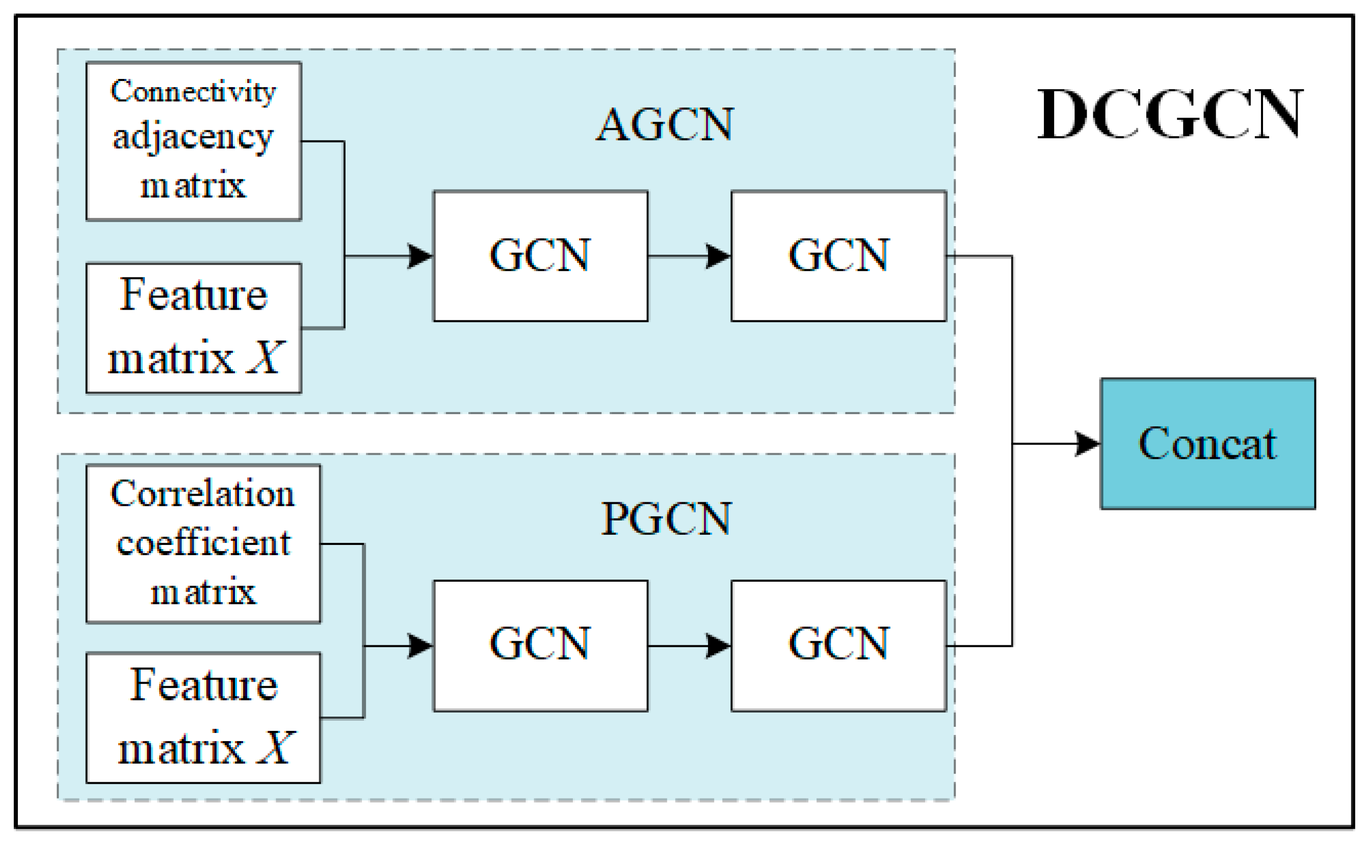
Figure 3 indicates that there is a spatial correlation between different network nodes. It is further seen that the nodes with connectivity to A (i.e., B, C, D, E) have different spatial correlations to the target node A. There are nodes with correlation coefficients less than 0.9, and nodes that are not connected to point A with correlation coefficients greater than 0.9. The spatial correlations between the nodes with connectivity to A (i.e., B, C, D, E) and the target node A are different. Therefore, merely setting the connectivity neighborhood matrix is not enough to describe the spatial dependency of the traffic network. In this paper, a new DCGCN model is proposed as presented in Figure 4.

The DCGCN model is built on top of the basic GCN model, which consists of the AGCN and the PGCN, and the results after Concat are:

$$f(X,A,P)=[f(X,A)|f(X,P)]$$

(11)

where $|$ represents the stitching of the matrix, the adjacency matrix of the AGCN is set to the connectivity adjacency matrix described above, and the adjacency matrix of the PGCN is replaced by the Pearson correlation coefficient matrix. This matrix is fused with the features extracted by the adjacency feature extraction module to capture the connectivity between nodes, and the spatial correlation, respectively.

3.3. Temporal Feature Modeling

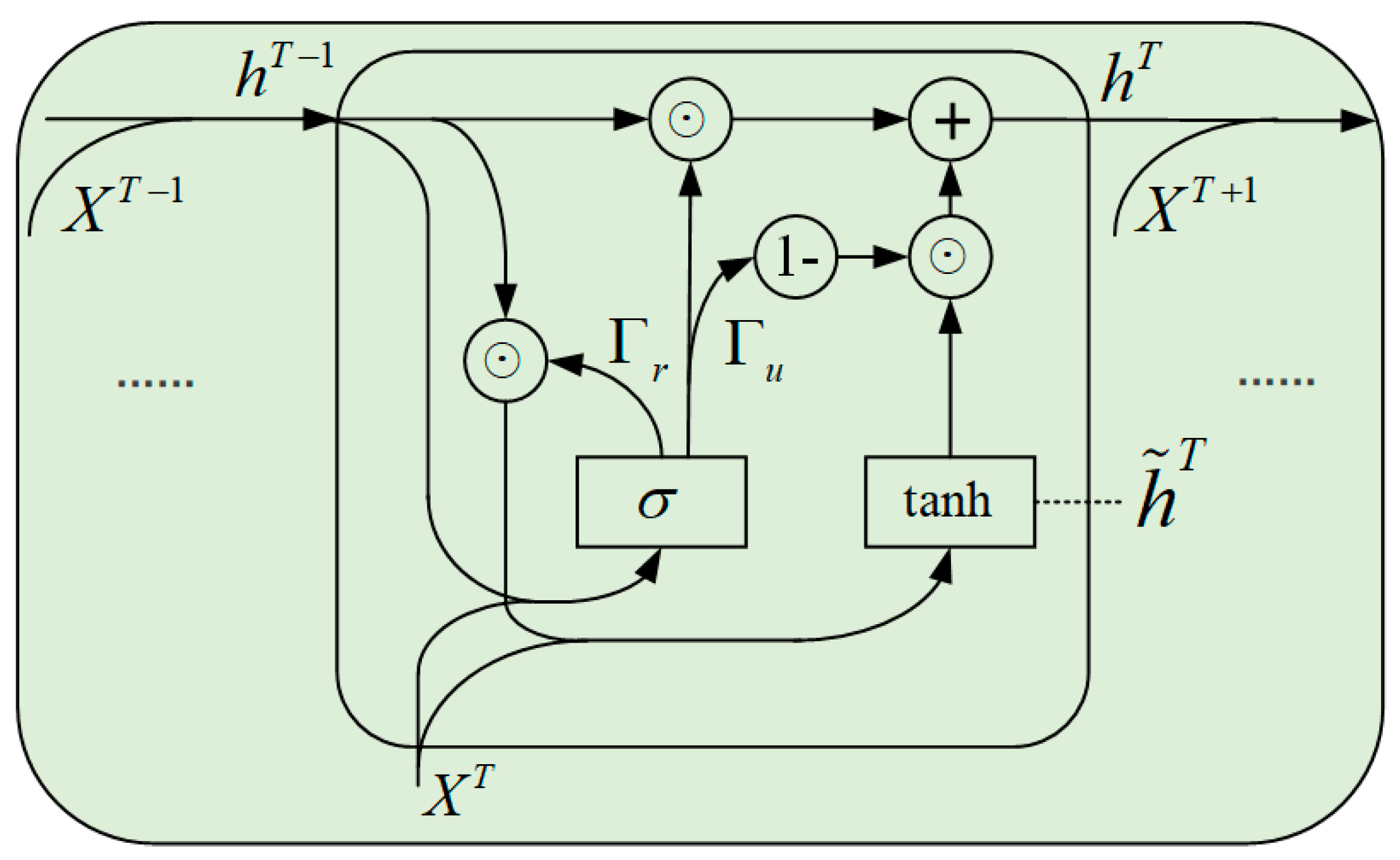
The most commonly used model for extracting the temporal characteristics of natural sequences is the RNN. However, as the time series becomes too long and the input information becomes larger, training RNN to converge to a global optimum becomes a challenging task. The GRU and LSTM are special recurrent neural networks that alter the hidden layers of RNN to better capture the deep connections and effectively improve the problem of gradient disappearance due to long sequences [25]. Note that the internal structure of the GRU is simpler and the training time is shorter than that of the LSTM. Therefore, the GRU model is used in this paper to extract the temporal characteristics of network traffic. The structure of the considered GRU is shown in Figure 5, where $h^{t-1}$ denotes the hidden state at the time $t-1$ and $X^t$ denotes the traffic characteristics of at $t$. The $t$ hidden states of a moment $h^t$ are determined using an update gate ${\Gamma }_u$ that determines whether the hidden state of the previous moment $h^{t-1}$ is maintained or it is updated to a candidate hidden state of the moment ${\tilde{h}}^t$, ${\Gamma }_u$ using $\sigma$, a function that makes itself equal to a value approximately equal to 0 or 1. Note that ${\Gamma }_r$ is a reset gate to control the extent to which the previous status message $h^{t-1}$ is ignored. The structure of the GRU enables capturing long-range dependencies and is well suited for extracting the temporal characteristics of long correlation sequences, which is typical for predicting network traffic over time.

3.4. DC-STGCN Model

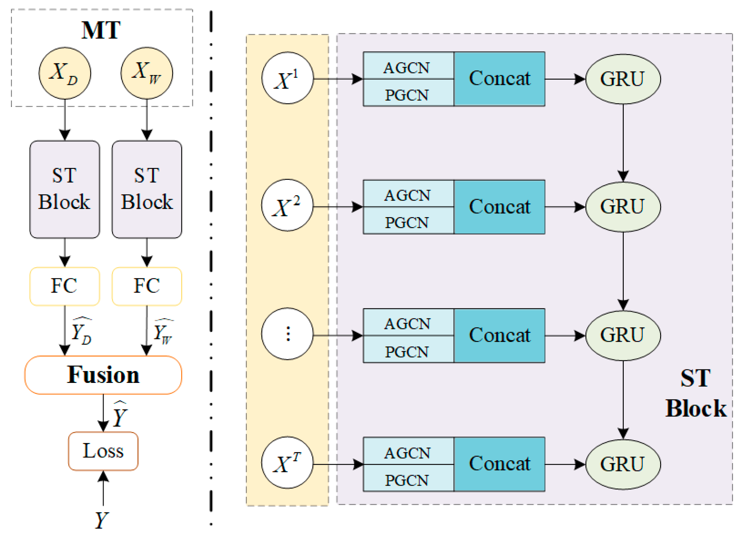
To better extract the spatiotemporal characteristics of the traffic data, a DC-STGCN model is proposed in this paper based on the GCN and the GRU. The structure of this model is shown in Figure 6. It mainly consists of a Multitime Component Input (MT), a Spatial-temporal Feature Extraction Unit (ST-Block), and a Feature Fusion.

3.4.1. Multitime Component Input

The network traffic at the current moment is affected by the previous moment, as explained in the Section 1. Daily periodicity means that the network traffic of the past few days affects the traffic of the current day, while weekly periodicity means that the current traffic is similar to the traffic of the same moment in the past few weeks. Therefore, this paper uses these two different scales of MT to capture the effects of the daily and weekly periodicity of traffic. This further enriches the model’s extraction of the temporal characteristics of the traffic. As shown in Figure 7, assuming a daily input with a time window of length $f$, the model has a daily cycle input $X_D=[x^{(t-d*f)},\cdots ,x^{(t-f)}]$, a weekly cycle input $X_W=[x^{(t-7*w*f)},\cdots ,x^{(t-7*f)}]$, and then predicts the flow in time $Y$.

3.4.2. Spatial-Temporal Feature Extraction Unit

On the right side of Figure 6 is a spatiotemporal feature extraction unit that consists of DCGCN and GRU. The spatial features of the historical time series are extracted from the DCGCN and the temporal features are input into the GRU. Furthermore ${\Gamma }_r$ is the hidden state at the time of $t$, and ${\Gamma }_u$ ${\Gamma }_r$ are the update, and reset gates, respectively. The following equations show the calculation process, where $f(X^t,A,P)$ is the output of the spatial feature extracted from the DCGCN input for the moment t, $W_{u,r,c}$ and $b_{u,r,c}$ are the weight, and bias terms, respectively.

$${\Gamma }_u=\sigma (W_u[f(X^t,A,P),h^{t-1}]+b_u)$$

(12)

$${\Gamma }_r=\sigma (W_r[f(X^t,A,P),h^{t-1}]+b_r)$$

(13)

$${\tilde{h}}^t=\tanh (W_c[f(X^t,A,P),({\Gamma }_r*h^{t-1})]+b_c)$$

(14)

$$h^t={\Gamma }_u*{\tilde{h}}^t+(1-{\Gamma }_u)*h^{t-1}$$

(15)

3.4.3. Feature Fusion

The degree to which the characteristics of the inputs in different scales affect the prediction results varies. For example, if the peak and trough values of traffic at some network nodes are in a time pattern, and the daily traffic is less mutable, the daily cycle input and the weekly cycle input are important for the prediction results. Therefore, the predictions are learned from the inputs of the temporal components at different time scales, and the final result of the fusion is:

$$\widehat{Y}=P_1\odot \widehat{Y_D}+P_2\odot \widehat{Y_W}$$

(16)

where $\odot$ is the Hadamard multiplier, and $P_1$, $P_2$ indicate the extent to which daily, and weekly cycle inputs influence the prediction results, respectively.

4. Experimental Implementation and Analysis

4.1. Data Description

To verify the validity of the model, an open dataset was chosen as the experimental dataset in this paper. This dataset contained the network traffic network data collected in the city of Milan [26]. The sampling frequency of the dataset was 10 min/time, i.e., one day contains 144 Sampling points. Two arrays of nine regions were selected for model evaluation: (1) Working Days: 1 November 2013–29 November 2013; (2) Holidays: 3 November 2013–1 December 2013.

The first 80% of each data set was used as the training set, and 10% of the data in the training set was used as the validation set for the initial training. After the best model was saved, the complete training set was used for further training, and the last 20% of the data was used as the test set. Before the prediction, the sample data was normalized using the MinMaxScaler function. This standardized the data in the $[0,1]$ interval and the reverse normalization was carried out before outputting the results.

4.2. Evaluation Indicators

To fully validate the predictive accuracy of the model, as the data are sampled at an interval of 10 min, we used 10 min (1 point), 20 min (2 points), and 30 min (3 points) for single and multistep forecasting respectively. Besides, three evaluation metrics were selected as indicators to judge the effectiveness of the model as the following.

1

Root Mean Square Error (RMSE), which reflects the prediction error of the model. The error value is $\left[0,+\infty \right]$ in the range. The closer the error to zero, the better the model. The formula is as follows.

$$RMSE=\sqrt{\frac{1}{T}{\displaystyle \sum _{t=1}^T(y_{\mathrm{true}}^t-y_{\mathrm{pred}}^t})}$$

(17)

2

Accuracy reflects the accuracy of a model’s predictions. The range of accuracy is $\left[0,1\right]$. The closer the value of Accuracy to 1, the better the model. Which is defined as follows:

$$\mathrm{Accuracy}=1-\frac{{\displaystyle \sum _{t=1}^T\left|y_{\mathrm{true}}^t-y_{\mathrm{pred}}^t\right|}}{{\displaystyle \sum _{t=1}^T{y}_{\mathrm{true}}^t}}$$

(18)

3

Coefficient of Determination ($R^2$ score): the value of $R^2$ indicates the degree of model excellence. The evaluation criterium is the same as for the accuracy:

$$R^2=1-\frac{{\displaystyle \sum _{t=1}^T{(y_{\mathrm{true}}^t-y_{\mathrm{pred}}^t)}^2}}{{\displaystyle \sum _{t=1}^T{(y_{\mathrm{ave}}^t-y_{\mathrm{pred}}^t)}^2}}$$

(19)

where $y_{\mathrm{true}}^t$ and $y_{\mathrm{pred}}^t$ denote the actual and predicted values at the time $t$, respectively, $y_{\mathrm{ave}}^t$ denotes the mean value of the data samples, and $T$ is the number of samples.

4.3. Parameter Design

In this study, we used the Python 3.7 programming environment. The network framework was built using TensorFlow, and the operating system was Windows 10 64bit. The computer included an Intel(R) Core(TM) i7-9700CPU @ 3.00 GHz processor, with 32 GB RAM. And the equipment was purchased from Dell in Nanjing, China.

In this experiment, Adam was chosen as the optimizer, the learning rate was set to 0.001, the epoch for model training was 2000, and the minibatch size was 16. The sliding window $L$ is equivalent to a slider sliding on the top of a scale with a specified length. Each unit sliding gives feedback on the data within the slider and that is the predicted data. The number of hidden cells $H$ is the number of neurons in the input GRU. There are important hyperparameters that affect the precision of the prediction results. In this paper, we compared the accuracy and $R^2$ of the prediction results to determine the optimal values of $L$ and $H$.

In this experiment, the length $L$ of the sliding window was set to $[4,8,12,16]$. Figure 8 and Figure 9 show the changes in the accuracy and $R^2$ on the two datasets of working days and holidays. As is seen the changes in both indicators of accuracy and $R^2$ were largely consistent and correlated. For the working days, Figure 8a shows that the Accuracy and $R^2$ values were the highest for the sliding window length of 8; conversely, for the holidays, as shown in Figure 8b, the accuracy and $R^2$ value were the highest for the sliding window length of 12. To select the best sliding window, a new dataset with both working day and holiday test sets was adopted. And the sliding window length $L$ was set to $[4,6,8,10,12,14,16]$ (

Table 1. Prediction results for different length sliding windows.

Sliding Window Length	10 min
	RMSE	Accuracy	${\mathit{R}}^2$
4	5.5251	0.7113	0.8054
6	5.4431	0.7166	0.8133
8	5.4145	0.7174	0.8141
10	5.4495	0.7162	0.8135
12	5.4609	0.7158	0.8135
14	5.4908	0.7140	0.8118
16	5.4959	0.7137	0.8113

).

As seen in Table 1, the best results were obtained at $L=8$. Besides, as the sliding window length increased, the difficulty of calculation increased and the prediction accuracy decreased. Therefore, this paper used $L=8$ as the length of the sliding window, i.e., 8 historical network traffic data ($X^t,X^{t+1},\cdots \cdots ,X^{t+7}$) to predict the future traffic.

For the selection of the $H$ number of hidden layers, we considered $(8,16,32,64,128)$. Figure 9a,b show the values of accuracy and $R^2$ for different numbers of hidden layers on the two datasets. It is seen that for both datasets, accuracy and $R^2$ were at their maximum values for $H$ = 64; therefore $H$ was set to 64 in this experiment.

4.4. Experimental Results

A comparison of DC-STGCN with the following traditional timing prediction models and machine learning models was performed and the results are presented in

Table 2. The comparison results between the DC-STGCN and other baseline models.

Models		10 min			20 min			30 min
		RMSE	Accuracy	${\mathit{R}}^2$	RMSE	Accuracy	${\mathit{R}}^2$	RMSE	Accuracy	${\mathit{R}}^2$
Working Day	HA	3.790	0.812	0.898	3.790	0.812	0.898	3.790	0.812	0.898
	ARIMA	4.951	0.634	*	4.997	0.631	*	5.022	0.629	*
	SVR	3.728	0.815	0.901	3.888	0.813	0.899	4.085	0.804	0.889
	GRU	3.703	0.822	0.909	3.694	0.822	0.908	3.850	0.816	0.901
	T-GCN [2]	3.441	0.824	0.911	3.593	0.824	0.910	3.734	0.819	0.902
	[3]	-	-	-	-	-	-	-	-	-
	DC-STGCN	3.232	0.844	0.933	3.394	0.840	0.920	3.621	0.832	0.909
Holiday	HA	4.190	0.790	0.835	4.190	0.790	0.835	4.190	0.790	0.835
	ARIMA	5.094	0.635	*	5.094	0.635	*	5.116	0.634	*
	SVR	4.243	0.788	0.835	4.326	0.780	0.831	4.333	0.780	0.821
	GRU	4.115	0.799	0.841	4.129	0.799	0.840	5.406	0.751	0.811
	T-GCN [2]	3.827	0.805	0.855	4.121	0.794	0.835	4.130	0.789	0.831
	DC-STGCN	3.791	0.815	0.866	3.881	0.807	0.854	3.910	0.805	0.852

* the resultant data that can be ignored.

.

HA: historical average model, which uses historical averages as predictions. Here we used the average of the last eight time samples to predict the value at the next moment.

ARIMA: autoregressive integrated moving average model, one of the most widely used predictive models for time series.

SVR: supports vector regression model, for which the prediction results were obtained by training based on historical data. SVR has the advantage of fewer training parameters and better results. In this paper, a linear kernel function was used and the penalty factor set to 0.001.

GRU: gated recurrent unit, a variant of the RNN, which is an efficient solution to the gradients vanishing issue after a long sequence of inputs.

In this experiment, Table 2 shows the prediction results for the next 10, 20, and 30 min for different models on different data sets (working days, holidays). The models were trained five times and then averaged for the final results. As the value of ARIMA was too small, * represents the resultant data that can be ignored. Analysis of Table 2 indicates the following:

(1)

The DC-STGCN model had the best forecast error, forecast precision, and correlation coefficient. For example, for a forecast step of 10 min on the working day dataset, the accuracy and $R^2$ values for DC-STGCN were, respectively, 3.2% and 3.5% higher than that of the HA model, and the RMSE was reduced by 0.558. Compared to the ARIMA model, the RMSE and accuracy of DC-STGCN were, respectively, 1.719 lower and 21.0% higher. While the accuracy and $R^2$ of DC-STGCN were improved by 2.9% and 3.2% compared to the SVR, the prediction was poorer as the SVR used a linear kernel function. It can be further seen that the neural network-based models, both DC-STGCN and GRU, outperformed the other models. This is because of the poor fit provided by the HA and ARIMA to such a long series of unsteady data, whereas the neural network models fitted the nonlinear data much better.

(2)

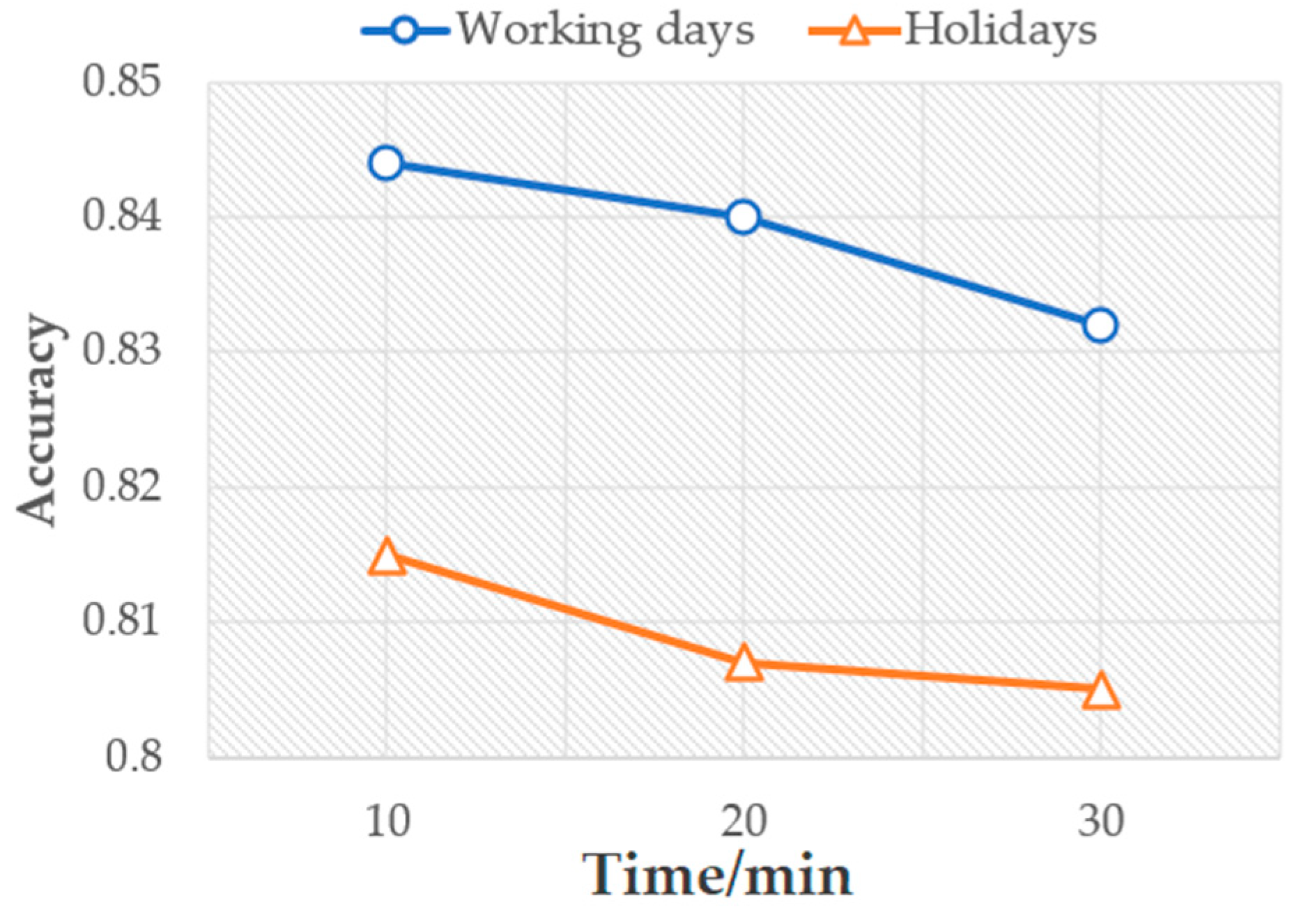
The DC-STGCN model had long-term forecasting capability. By increasing the prediction time, the prediction performance of the DC-STGCN model was decreased. Nevertheless, the DC-STGCN model still had the best prediction performance comparing with the other models. Figure 10 shows the change in accuracy with increasing forecast time for the DC-STGCN model on both working day and holiday datasets. The accuracy decreased with the forecast time, but the downward trend was rather smooth. Therefore, the DC-STGCN model was less affected by forecast time and had stable long-term forecasting capability.

(3)

Network traffic is cyclical as well as self-similar [11]. The network traffic at the current moment is affected by the previous moment. Therefore, in this paper, we used two different scales of MT to capture the effects of the daily and weekly periodicity of traffic. In contrast, the model proposed by He et al. [5] didn’t take into account the flow characteristic; therefore, the DC-STGCN could extract a richer temporal feature. Meanwhile, the results in Table 2 suggest that the DC-STGCN model predicted better than the model (T-GCN), proposed by Zhao et al. [4].

(4)

Comparing the prediction results of the working day and holiday datasets, the DC-STGCN model predicted network traffic better on the working day dataset than the holiday dataset. This is because holiday network traffic peaks are higher than weekday peaks and the traffic, therefore, is harder to predict. The DC-STGCN model predicted traffic more accurately for the working day dataset than the holiday dataset. This is because, unlike the more regular weekday traffic, the network traffic on holidays is more random.

4.5. Ablation Studies

To verify the advanced nature of the DC-STGCN model, this section validates the effectiveness of the two modules proposed in this paper. The effectiveness of the modules including DC (dual-channel GCN) and MT (Multi-time Component Input) were investigated through ablation experiments. Based on the single-channel GCN-GRU model, the modules (1) DC; (2) MT; and (3) DC+MT (the proposed model in this paper) were added in turn, resulting in three submodels for multistep prediction on the working day dataset. The results are presented in Figure 11.

It can be seen that the prediction precision of the submodel with the MT module was higher than that of the submodel with the DC module. Nevertheless, the prediction performance of the sub-model with the MT module was significantly decreased by increasing the prediction time. This suggests that this setting was not suitable for long-term prediction. The submodel with the DC module was stable in multistep forecasting, but as network traffic is typically a time series, its temporal characteristics affected the prediction precision of the model more than its spatial characteristics. The submodel with the MT module extracted richer temporal characteristics of the network traffic, so the overall prediction of the submodel with the DC module alone was inferior. The model with the DC+MT module (the DC-STGCN model) combined the advantages of both modules, and it can be seen that the DC-STGCN model not only provided high prediction precision but was suitable for multistep prediction.

The ablation experiments confirmed that the DC and MT modules proposed in this paper are effective. The DC module enabled the DC-STGCN model to capture the connectivity between the nodes, and the near-correlation, hence extracting richer spatial features. Furthermore, the DC-STGCN model used the MT module to capture the daily and weekly flow periodicity, further enriching the model’s extraction of the temporal features of the flow. The results in Table 2 also indicate that the DC-STGCN model achieved the best prediction error, prediction accuracy and correlation coefficient on both examined datasets. These results suggest that the DC-STGCN model proposed in this paper is effective and achieves accurate and stable long-term prediction capability.

4.6. Model Interpretation

To better understand the DC-STGCN model, this section explores the differences in the model’s predictions on different datasets. We selected two network nodes on the working day and holiday datasets, respectively. We then visually compare the results of their one-step predictions with true values in Figure 12 and Figure 13.

(1) Network traffic is more regular on weekdays, starting to rise as people go to work (at or around 7 am), sampling point 42, reaching its peak for the day (at 5 pm), sampling point 102, and then falling as the users leave work, and eventually reaching a minimum in the early hours of the morning.

(2) Network traffic on holidays is more complex and variable than that of the weekdays. As it is seen on the left side of Figure 13 that holidays traffic is more random and unpredictable from 08:00 AM (point 48) onwards, depending on people’s lifestyles. On the right side of Figure 13, it is also seen that the holidays traffic is more likely to have sudden points of variation. The GCN model used a smooth filter moving in the Fourier domain to interact with the signal. This resulted in smoother predictions of the mutation regions so that the DC-STGCN model did not predict the datasets with multiple mutation points as well.

In summary, the DC-STGCN model had a lower prediction precision for holidays than for working days, but the prediction of trends in actual network traffic was almost identical. This indicates that the DC-STGCN model can accurately predict upcoming congestion events.

5. Conclusions

In this paper, we propose a DC-STGCN model consisting of two temporal components that characterize the daily and weekly correlation of network traffic. Each component contains a spatial-temporal feature extraction module consisting of a DCGCN-GRU model. The DCGCN consists of the AGCN and PGCN, and their adjacency matrices are set as connectivity adjacency matrices, and correlation coefficient matrices, respectively, which are used to extract the connectivity and proximity correlation between nodes. In our proposed method, the GRU extracts the temporal characteristics of the traffic. Trained on two real datasets, the results show that the proposed model outperformed existing models in terms of prediction error, prediction precision, and correlation coefficient, and could make long-term predictions. Compared to the traditional ARIMA model, the DC-STGCN model with a forecast length of 10 min on the working day dataset reduced the RMSE and accuracy by 1.719, and improved it by 21%, respectively, with significantly better forecasting performance. In the future, we may consider the construction of multitask prediction models, such as the simultaneous prediction of traffic rates and throughput.

References

1. Feng, J.; Chen, X.; Gao, R.; Zeng, M.; Li, Y. DeepTP: An End-to-End Neural Network for Mobile Cellular Traffic Prediction. IEEE Netw. 2018, 32, 108–115. [Google Scholar] [CrossRef]
2. Andreoletti, D.; Troia, S.; Musumeci, F.; Giordano, S.; Maier, G.; Tornatore, M. Network Traffic Prediction based on Diffusion Convolutional Recurrent Neural Networks. In Proceedings of the IEEE INFOCOM 2019—IEEE Conference on Computer Communications Workshops (INFOCOM WKSHPS), Paris, France, 29 April–2 May 2019; IEEE: Piscataway, NJ, USA, 2019; pp. 246–251. [Google Scholar]
3. Yang, L.; Gu, X.; Shi, H. A Noval Satellite Network Traffic Prediction Method Based on GCN-GRU; WCSP: Nanjing, China, 2020; pp. 718–723. [Google Scholar]
4. Zhao, L.; Song, Y.; Zhang, C.; Liu, Y.; Wang, P.; Lin, T.; Deng, M.; Li, H. T-GCN: A Temporal Graph Convolutional Network for Traffic Prediction. IEEE Trans. Intell. Transp. Syst. 2020, 21, 3848–3858. [Google Scholar] [CrossRef] [Green Version]
5. He, K.; Huang, Y.; Chen, X.; Zhou, Z.; Yu, S. Graph Attention Spatial-Temporal Network for Deep Learning Based Mobile Traffic Prediction. In Proceedings of the 2019 IEEE Global Communications Conference (GLOBECOM), Waikoloa, HI, USA, 9–13 December 2019; Institute of Electrical and Electronics Engineers (IEEE): Piscataway, NJ, USA, 2019; pp. 1–6. [Google Scholar]
6. Guo, S.; Lin, Y.; Feng, N.; Song, C.; Wan, H. Attention Based Spatial-Temporal Graph Convolutional Networks for Traffic Flow Forecasting. In Proceedings of the AAAI Conference on Artificial Intelligence; Association for the Advancement of Artificial Intelligence (AAAI): Menlo Park, CA, USA, 2019; Volume 33, pp. 922–929. [Google Scholar]
7. Ahmed, M.S.; Cook, A.R. Analysis of Freeway Traffic Time-Series Data by Using Box-Jenkins Techniques. Transportation Research Record: Thousand Oaks, CA, USA, 1979. [Google Scholar]
8. Laner, M.; Svoboda, P.; Rupp, M. Parsimonious Fitting of Long-Range Dependent Network Traffic Using ARMA Models. IEEE Commun. Lett. 2013, 17, 2368–2371. [Google Scholar] [CrossRef]
9. Madan, R.; Mangipudi, P.S. Predicting Computer Network Traffic: A Time Series Forecasting Approach Using DWT, ARIMA and RNN. In Proceedings of the 2018 Eleventh International Conference on Contemporary Computing (IC3), Noida, India, 2–4 August 2018; Institute of Electrical and Electronics Engineers (IEEE): Piscataway, NJ, USA, 2018; pp. 1–5. [Google Scholar]
10. Qian, Y.; Xia, J.; Fu, K.; Zhang, R. Network traffic forecasting by support vector machines based on empirical mode decomposition denoising. In Proceedings of the 2012 2nd International Conference on Consumer Electronics, Communications and Networks (CECNet), Yichang, China, 21–23 April 2012; pp. 3327–3330. [Google Scholar]
11. Bie, Y.; Wang, L.; Tian, Y.; Hu, Z. A Combined Forecasting Model for Satellite Network Self-Similar Traffic. IEEE Access 2019, 7, 152004–152013. [Google Scholar] [CrossRef]
12. Ramakrishnan, N.; Soni, T. Network Traffic Prediction Using Recurrent Neural Networks. In Proceedings of the 2018 17th IEEE International Conference on Machine Learning and Applications (ICMLA), Orlando, FL, USA, 17–20 December 2018; Institute of Electrical and Electronics Engineers (IEEE): Piscataway, NJ, USA, 2018; pp. 187–193. [Google Scholar]
13. Tudose, A.M.; Sidea, D.O.; Picioroaga, I.I.; Boicea, V.A.; Bulac, C. A CNN Based Model for Short-Term Load Forecasting: A Real Case Study on the Romanian Power System. In Proceedings of the 2020 55th International Universities Power Engineering Conference (UPEC), Torino, Italy, 1–4 September 2020; Institute of Electrical and Electronics Engineers (IEEE): Piscataway, NJ, USA, 2020; pp. 1–6. [Google Scholar]
14. Zhang, Q.; Jin, Q.; Chang, J.; Xiang, S.; Pan, C. Kernel-Weighted Graph Convolutional Network: A Deep Learning Approach for Traffic Forecasting. In Proceedings of the 2018 24th International Conference on Pattern Recognition (ICPR), Beijing, China, 20–24 August 2018; Institute of Electrical and Electronics Engineers (IEEE): Piscataway, NJ, USA, 2018; pp. 1018–1023. [Google Scholar]
15. Nie, L.; Jiang, D.; Guo, L.; Yu, S.; Song, H. Traffic Matrix Prediction and Estimation Based on Deep Learning for Data Center Networks. J. Netw. Comput. Appl. 2016, 76, 16–22. [Google Scholar] [CrossRef]
16. Sebastian, K.; Gao, H.; Xing, X. Utilizing an Ensemble STL Decomposition and GRU Model for Base Station Traffic Forecasting. In Proceedings of the 2020 59th Annual Conference of the Society of Instrument and Control Engineers of Japan (SICE), Chiang Mai, Thailand, 23–26 September 2020; Institute of Electrical and Electronics Engineers (IEEE): Piscataway, NJ, USA, 2020; pp. 314–319. [Google Scholar]
17. Li, T.; Hua, M.; Wu, X. A Hybrid CNN-LSTM Model for Forecasting Particulate Matter (PM2.5). IEEE Access 2020, 8, 26933–26940. [Google Scholar] [CrossRef]
18. Bruna, J.; Zaremba, W.; Szlam, A.; Lecun, Y. Spectral Networks and locally connected networks on graphs. arXiv 2013, arXiv:1312.6203. [Google Scholar]
19. Gao, J.; Zhang, T.; Xu, C. I Know the Relationships: Zero-Shot Action Recognition via Two-Stream Graph Convolutional Networks and Knowledge Graphs. In Proceedings of the AAAI Conference on Artificial Intelligence, Honolulu, HI, USA, 27 January–1 February 2019; Association for the Advancement of Artificial Intelligence (AAAI): Menlo Park, CA, USA, 2019; Volume 33, pp. 8303–8311. [Google Scholar]
20. Zhu, J.W.; Song, Y.J.; Zhao, L.; Li, H.F. A3T-GCN: Attention Temporal Graph Convolutional Network for Traffic Forecasting. arXiv 2020, arXiv:2006.11583. [Google Scholar]
21. Lu, B.; Gan, X.; Jin, H.; Fu, L.; Zhang, H. Spatiotemporal Adaptive Gated Graph Convolution Network for Urban Traffic Flow Forecasting. In Proceedings of the 29th ACM International Conference on Information & Knowledge Management, Galway, Ireland, 19–23 October 2020; ACM: New York, NY, USA, 2020; pp. 1025–1034. [Google Scholar]
22. Ye, J.; Zhao, J.; Ye, K.; Xu, C. Multi-STGCnet: A Graph Convolution Based Spatial-Temporal Framework for Subway Passenger Flow Forecasting. In Proceedings of the 2020 International Joint Conference on Neural Networks (IJCNN), Glasgow, UK, 19–24 July 2020; Institute of Electrical and Electronics Engineers (IEEE): Piscataway, NJ, USA, 2020; pp. 1–8. [Google Scholar]
23. Defferrard, M.; Bresson, X.; Vandergheynst, P. Convolutional Neural Networks on Graphs with Fast Localized Spectral Filtering. In Proceedings of the NIPS’16 30th International Conference on Neural Information Processing Systems, Barcelona, Spain, 5–10 December 2016; pp. 3844–3852. [Google Scholar] [CrossRef]
24. Kipf, T.N.; Welling, M. Semi-Supervised Classification with Graph Convolutional Networks. arXiv 2017, arXiv:160902907. [Google Scholar]
25. Zhang, J.; Chi, Y.; Xiao, L. Solar Power Generation Forecast Based on LSTM. In Proceedings of the 2018 IEEE 9th International Conference on Software Engineering and Service Science (ICSESS), Beijing, China, 23–25 November 2018; Institute of Electrical and Electronics Engineers (IEEE): Piscataway, NJ, USA, 2018; pp. 869–872. [Google Scholar]
26. Barlacchi, G.; De Nadai, M.; Larcher, R.; Casella, A.; Chitic, C.; Torrisi, G.; Antonelli, F.; Vespignani, A.; Pentland, A.P.; Lepri, B. A multi-source dataset of urban life in the city of Milan and the Province of Trentino. Sci. Data 2015, 2, 150055. [Google Scholar] [CrossRef] [PubMed] [Green Version]
Figure 1. Spatial dependency diagram for network traffic.
Electronics 10 01014 g001
Figure 2. The temporal dependency diagram for network traffic. (a) The weekly trend. (b) The daily trend.
Electronics 10 01014 g002
Figure 3. The heat map of correlation coefficients for the network node traffic.
Electronics 10 01014 g003
Figure 4. Diagram of the DCGCN model results.
Electronics 10 01014 g004
Figure 5. Model structure of the GRU.
Electronics 10 01014 g005
Figure 6. The structure of the DC-STGCN model.
Electronics 10 01014 g006
Figure 7. An example structure for the MT.
Electronics 10 01014 g007
Figure 8. Performance comparison for different values of the sliding window lengths (a) Changes in accuracy and R 2 based on working days; (b) Changes in accuracy and R 2 based on holidays.
Electronics 10 01014 g008
Figure 9. Performance comparison for different numbers of the hidden layers. (a) Changes in accuracy and R 2 , based on working days. (b) Changes in accuracy and R 2 based on holidays.
Electronics 10 01014 g009
Figure 10. The plot of the results of the multistep prediction of the DC-STGCN model.
Electronics 10 01014 g010
Figure 11. Diagram of the predicted results of the two sub-models.
Electronics 10 01014 g011
Figure 12. Visualization of one-step prediction results for the working day dataset.
Electronics 10 01014 g012
Figure 13. Visualization of one-step prediction results for the holiday dataset.
Electronics 10 01014 g013