Abstract
Graphs are used as models to solve problems in fields such as mathematics, computer science, physics, and chemistry. In particular, torus, hypercube, and star graphs are popular when modeling the connection structure of processors in parallel computing because they are symmetric and have a low network cost. Whereas a hypercube has a substantially smaller diameter than a torus, star graphs have been presented as an alternative to hypercubes because of their lower network cost. We propose a novel log star (LS) that is symmetric and has a lower network cost than a star graph. The LS is an undirected, recursive, and regular graph. In LSn, the number of nodes is n! while the degree is 2log2n − 1 and the diameter is 0.5n(log2n)2 + 0.75nlog2n. In this study, we analyze the basic topological properties of LS. We prove that LSn is a symmetrical connected graph and analyzed its subgraph characteristics. Then, we propose a routing algorithm and derive the diameter and network cost. Finally, the network costs of the LS and star graph-like networks are compared.
1. Introduction
A graph consists of nodes and edges. The degree of a node u is the number of edges incident with u. The degree of a graph is the maximum degree over all nodes. The distance between two nodes u and v is the number of edges of the shortest path between u and v. The diameter of a graph is the maximum distance over all pairs of nodes. Graphs are used as models to solve problems in various fields. In computer science, graphs have been applied to the topology of parallel computers, the connection structure of very large-scale integrated (VLSI) internal cores, the connection structure of sink nodes and source nodes in wireless sensor networks (WSNs), and sorting problems. The measures for evaluating graphs vary depending on the field to suit the specific circumstances of each application. Smaller degrees and diameters are better for VLSI and parallel computers, which have a physical connection structure. In contrast, for sorting problems or WSNs with a logical connection structure, the diameter is a more important measure than the degree. In other fields, other evaluation measures may be more important [1]. In the interconnection network for parallel computing, since degree refers to the number of communication ports, the hardware installation cost increases when the degree increases. The diameter represents the length of the message transfer path between two processors, and when the diameter increases, the message transfer time increases, thus affecting the software cost. When the sorting algorithm is modeled as a graph, the diameter of the graph is an important measure because it is the worst time complexity of the sorting algorithm.
The evaluation measures of a graph include the number of nodes, number of edges, degree, diameter, network cost, bisection bandwidth, connectivity, symmetry, expandability, and fault tolerance. In addition, the answers to the following questions can be evaluated: Is it a regular graph? Is it a planar graph? Is it possible to embed it in another graph? Does it have a Hamiltonian path? Does it have a binary tree as a subgraph? Network cost and symmetry are also used as evaluation measures [2,3,4]. In this study, we propose a symmetric graph that has a lower network cost than a star graph.
The network cost of a graph is its degree × diameter. Minimizing the network cost is highly similar to the (d,k) problem and the packing density problem. These problems involve finding a graph that has a small degree and diameter. Graphs with a low network cost are advantageous in various applications. When a graph is applied, the degree is the initial setup cost, and the diameter is the cost of running the algorithm. When an edge is added to a graph, the degree increases, whereas the diameter decreases. Conversely, if an edge is removed, the degree decreases and the diameter increases. Because there is a trade-off between the degree and diameter, finding a graph with a low network cost is difficult [5,6].
In a symmetric graph, the topological properties of the graph are the same viewed from any point (node). Suppose that for any two nodes u and v in graph G, there is a bjiection that maps u onto v. Consider that G is node-transitive. If for any two edges (u, v) and (x, y) in G there exists a bijection that maps (u, v) onto (x, y), then G is edge-transitive. If G is node and edge-transitive, it is a symmetric graph. When a symmetric graph is applied, it provides a significant advantage: an evaluation measure that is analyzed or an algorithm that is created at an arbitrary node can be used at all other nodes. Examples of algorithms include routing, broadcasting, Hamiltonian cycle (path), and binary graph construction algorithms [4,7,8].
The star graph in Figure 1a was introduced as an alternative to the well-known hypercube because of its excellent network cost. In star graph, each node S1S2S3 … Sk−1SkSk+1 … S2k−1S2kS2k+1 … Sn−2Sn−1Sn is connected to nodes SkS2S3 … Sk−1S1Sk+1 … S2k−1S2kS2k+1 … Sn−2Sn−1Sn (2 ≤ k ≤ n). A hypercube Qn has a diameter of n, degree of n, and 2n nodes. The star graph Sn has a diameter of 1.5n − 2, a degree of n − 1, and n! nodes. The network cost of both graphs is O(n2). Thus, for a network cost on the same order, the number of nodes in the hypercube increases by a factor of two, whereas the number of nodes in the star graph increases by a factorial linear arrangement. The star graph is therefore superior to the hypercube in terms of the network cost per node. Star graph-like networks include stars [9], hyper stars [10], macro stars [11], matrix stars [12], bubble sort [13], and hierarchical stars [14].
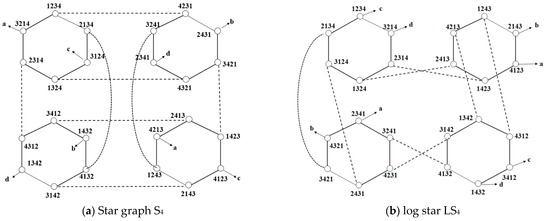
Figure 1.
Four-dimensional star S4 and log star LS4.
In this study, we propose a symmetric log star graph that has a lower network cost than a star graph. In Section 2, the notation used throughout the paper is listed, and the log star is defined. In Section 3, we analyze the basic topological properties, symmetry, subgraphs, and connectivity of log stars. In Section 4, we present a routing algorithm and analyze the diameter and network cost, which we compare with the network cost of star graph-like networks. Finally, in Section 5, we present our conclusions.
2. Notation and Definition of the Log Star
In this section, we provide the definitions used in this paper, and we define the log star LSn. The node address of LSn uses a permutation of the natural numbers from 1 to n. Let an arbitrary node be S = S1S2S3 … Sk−1SkSk+1 … S2k−1S2kS2k+1 … Sn−2Sn−1Sn. In Definition 2, the symbols s1 and Sk are exchanged with each other, and in Definition 3, multiple symbols are exchanged.
Definition 1.
Sk is the k-th symbol, s1 is the most significant bit (MSB), and Sn is the least significant bit (LSB).
Definition 2.
The exchange operation for S is EOk(S) = SkS2S3 … Sk−1S1Sk+1 … S2k−1S2kS2k+1 … Sn−2Sn−1Sn, k = 20 + 1, 21 + 1, 22 + 1, ⋯, 2n/2 + 1.
Definition 3.
The swap operation for S is SOk(S) = Sk+1 … S2k−1S2kS1S2S3 … Sk−1Sks2k+1 … sn−2sn−1sn, k = 20, 21, 22, ⋯, 2n/2.
The definition of log star LSn is as follows.
LSn = (V, E) | n = 2m, where m is a natural number.
node V = { S1S2S3 … Sk−1SkSk+1 … Sn−2Sn−1Sn | 1 ≤ Sk ≤ n, 1 ≤ k ≤ n }.
The edges in LSn are divided into exchange edges (EEs) and swap edges (SEs) and are defined as follows:
Exchange edge EEk = (S, EOk(S)).
Swap edge SEk = (S, SOk(S)).
For example, in LS8, the (connected edge, neighboring node) pairs for node 12345678 are as follows:
Exchange edges: (EE2, 21345678), (EE3, 32145678), (EE5, 52341678).
Swap edges: (SE1, 21345678), (SE2, 34125678), (SE4, 56781234).
Figure 1b shows an LS4 where the solid lines within the hexagons are EEs, and the dotted lines connecting one hexagon to another are the SEs. Furthermore, SE1 and EE2 are the same edges.
A path can be expressed as a sequence of nodes from a start node to a destination node. In this case, the neighboring nodes are connected by edges. A path can be defined as follows:
The notation 1. → is used to indicate a path. For example, the path between 1234, 2134, 3421, and 4321 in Figure 1b can be represented as follows:
1234 → 2134 → 3421 → 4321 or
1234 → EE1 → 2134 → SE2 → 3421 → EE1 → 4321.
3. Topological Properties of the Log Star
Here, we examine the basic topological properties of the LS.
Theorem 1.
LSn is a regular graph with a degree of 2log2n − 1; its number of nodes is n!, and its number of edges is n!log2n − 0.5n.
Proof.
Since the node address of LSn is a permutation of the natural numbers from 1 to n, the total number of nodes is n!. At every node, the number of SEs is log2n, and the number of EEs is log2n. Since SE1 and EE2 are the same, the degree is 2log2n − 1. Because LSn has the same degree at each node, it is a regular graph. Further, it is an undirected graph, where the total number of edges is (n! × (2log2n − 1))/2 = n!log2n − 0.5n!. □
Two graphs with the same topology are called isomorphic, regardless of their shape. Consider the graphs G(V, E) and H(V, E) and the mapping functions f: V(G) → V(H) and g: E(G) → E(H). If bijections f and g exist, then G and H are isomorphic. Here, if f: V(G) → V(G) and g: E(G) → E(G), then graph G is automorphic and symmetric. This can be explained as follows: for any two nodes u and v of G, if there is a bijection that maps u to v, then G is a node-transitive graph. For any two edges (u, v) and (x, y) of G, if there is a bijection that maps (u, v) to (x, y), G is an edge-transitive graph. If G is both node and edge-transitive, it is a symmetric graph. It is well known that a permutation composed of natural numbers, as in a star graph, is a symmetry group [4] and that symmetry groups are automorphic. Since the nodes of LSn are permutations from 1 to n, LSn is a node-transitive graph. The proof of edge transitivity is provided in Theorem 2, and node transitivity is omitted.
Theorem 2.
LSn is a symmetric graph.
Proof.
Let an arbitrary node be S = S1S2S3 … Sk … Sn−1Sn. The mapping function is f = S1S2S3 … Si … Sn−1Sn → S1S2S3 … Si … SnSn−1. The mapping function f is a bijection, which can be any function that exchanges symbols. An edge that is connected to S is denoted by (S, T). It is shown that f(S) and f(T) are connected to each other.
First, consider the mapping of an EE:
If S = S1S2S3 … Sk … Sn−1Sn, then T = SKS2S3 … S1 … Sn−1Sn. f(S) = S1S2S3 … Sk … SnSn−1, and f(T) = SkS2S3 … S1 … SnSn−1. Thus, f(S) and f(T) are exactly connected with the EEk.
Next, consider the mapping of an SE:
If S = S1S2S3 … Sk−1SkSk+1 … S2k−1S2kS2k+1 … Sn−2Sn−1Sn, then T = Sk+1 … S2k−1S2kS1S2S3 … Sk−1SkS2k+1 … Sn−2Sn−1Sn. f(S) = S1S2S3 … Sk−1SkSk+1 … S2k−1S2kS2k+1 … Sn−2SnSn−1, and f(T) = Sk+1 … S2k−1S2kS1S2S3 … Sk−1SkS2k+1 … Sn−2SnSn−1. f(S) and f(T) are thus exactly connected to SEk. Therefore, LSn is a node and edge-transitive graph and is symmetric. □
If all the nodes of a graph are connected, it is a connected graph; that is, in a connected graph, there is a path from an arbitrary node to every other node in the graph. The node addresses are expressed as permutations. If the MSB can move to any other position, the opposite is also possible. Thus, it has been shown that LSn is a connected graph.
Theorem 3.
LSn is a connected graph.
Proof.
We examined LS4 and LS8 and generalized LSn above. Definitions 2 and 3 are used here. In LS4, S = S1S2S3S4. The movement of the MSB by SO is as follows:
S1S2S3S4 = S.
S2S1S3S4 = SO1(S).
S3S4S1S2 = SO2(S).
S3S4S2S1 = SO2(SO1(S)).
S2S1S3S4 = SO1(S).
S3S4S1S2 = SO2(S).
S3S4S2S1 = SO2(SO1(S)).
Therefore, LS4 is a connected graph. In LS8, S = s1s2s3s4s5s6s7s8. For LS4, it has been shown that the MSB can move to positions 2, 3, and 4. If SO4 is added, the MSB can move to positions 5, 6, 7, and 8. The movement of the MSB by SO is as follows:
S1S2S3S4 = S.
S2S1S3S4 = SO1(S).
S3S4S1S2 = SO2(S).
S3S4S2S1 = SO2(SO1(S)).
S5S6S7S8 S1S2S3S4 = SO4(S).
S5S6S7S8S2 S1S3S4 = SO4(SO1(S)).
S5S6S7S8S3S4 S1S2 = SO4(SO2(S)).
S5S6S7S8 S3S4S2 S1 = SO4(SO2(SO1(S))).
S2S1S3S4 = SO1(S).
S3S4S1S2 = SO2(S).
S3S4S2S1 = SO2(SO1(S)).
S5S6S7S8 S1S2S3S4 = SO4(S).
S5S6S7S8S2 S1S3S4 = SO4(SO1(S)).
S5S6S7S8S3S4 S1S2 = SO4(SO2(S)).
S5S6S7S8 S3S4S2 S1 = SO4(SO2(SO1(S))).
Therefore, LS8 is also a connected graph. In LSn, the MSB can move to positions 2, 3, 4, ⋯, n/2. If SOn/2 is added, the MSB can move to positions n/2 + 1, n/2 + 2, ⋯, n. Therefore, LSn is a connected graph. □
Let G = (V, E) and H = (V, E). If V(H) ⊆ V(G) and E(H) ⊆ E(G), H is called a subgraph of G. Consider subgraphs H1 and H2 of G. When V(H1) ∩ V(H2) = ∅ and E(H1) ∩ E(H2) = ∅, the two subgraphs are said to be both node and edge-disjoint. Disjoint subgraphs can be used for process allocation, load balancing, broadcasting algorithms, and disjoint paths. The disjoint subgraphs of LSn are presented below.
Theorem 4.
LSn consists of n!/(n/2)! subgraphs LSn/2. The number of nodes in the subgraphs is (n/2)!, and they are node- and edge-disjoint with each other.
Proof.
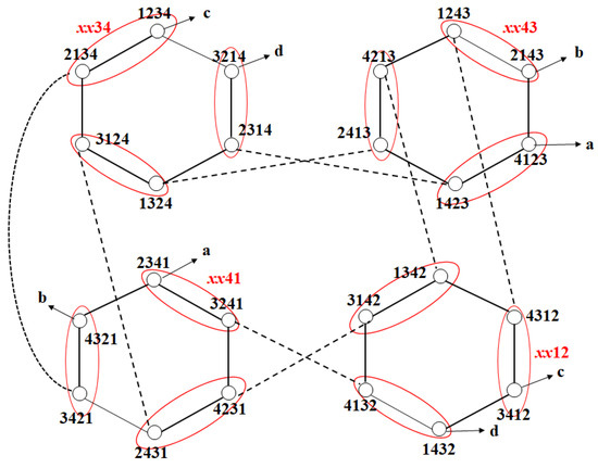
The number of nodes in LS4 is 4!. LS4 comprises 12 (=4!/2!) LS2. The number of nodes in LS2 is 2!. Figure 2 shows the subgraphs xx12, xx13, xx14, xx23, xx24, xx21, xx34, xx31, xx32, xx41, xx42, and xx43. x refers to an arbitrary number.
Figure 2.
Subgraphs of LS4.
The number of nodes in LS8 is 8!. LS8 consists of 8!/4! LS4, and the number of nodes in LS4 is 4!. The number of nodes in LSn is n!, and LSn consists of n!/(n/2)! LSn/2. The number of nodes in LSn/2 is (n/2)!. □
Theorem 5.
LSn comprises 2n!/n2 subgraphs. The subgraphs are both node and edge-disjoint, and the number of nodes is 0.5n2. All the subgraphs have Hamiltonian cycles and paths.
Proof.

First, LS4 and LS8 are examined, and then the result is generalized to LSn.
We first examine the subgraphs in LS4:
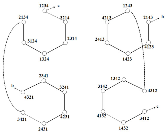
To define a subgraph, the natural numbers 1 to 4 used in the node addresses of LS4 are divided into two bundles, regardless of order. For example, they can be divided into bundles 12 and 34. There is no order inside a bundle. The node sets composed of these bundles are thus 1234, 2134, 1243, 2143, 3412, 3421, 4312, and 4321, which are shown as subgraphs (Figure 3). Note that the natural numbers could alternatively be divided into bundles 13 and 24 or 14 and 23. Consider the orange nodes in Figure 3, where the bundles 12 and 34 are not mixed; in the three subgraphs in Figure 3, the representative nodes are 1234, 1324, and 1423. We examine the path of repeating SE1 and SE2 four times at these nodes. This path is the Hamiltonian cycle of the subgraph, where the three cycles are represented by green, red, and orange. The number of nodes in a subgraph is 8. Because the numbers of the two bundles do not mix with each other in the SE operation, the three subgraphs are all node and edge-disjoint with each other. If the last SE2 is omitted, the path is a Hamiltonian path, which is used on LS8. If the start node of this path is s1s2s3s4, then the destination node is s3s4s1s2. The Hamiltonian sequence is HS4 = SE1 → SE2 → SE1 → SE2 → SE1 → SE2 → SE1.
Figure 3.
Subgraphs with a Hamiltonian cycle in LS4.
We now consider the subgraphs in LS8.
As for LS4, we examine the division of the natural numbers 1 to 8 into two bundles, where the within-bundle order is irrelevant. For example, suppose the numbers are divided into bundles 1234 and 5678; in this case, n is the number of subgraphs: (n × (n/2)) = (1 × 2 × 3 × 4 × 5 × 6 × 7 × 8) = 1260. We explain this by taking one subgraph as an example. If HS4 and SE4 are repeated four times at node 12345678, a cycle with a path length of 32 (=n × (n/2)) is created. The number of nodes in the subgraph is 32, and HS8 = HS4 → SE4 → HS4 → SE4 → HS4 → SE4 → HS4:
12345678 →
HS4 → 34125678 → SE4 → 56783412 →
HS4 → 78563412 → SE4 → 34127856 →
HS4 → 12347856 → SE4 → 78561234 →
HS4 → 56781234 → SE4 → 12345678.
HS4 → 34125678 → SE4 → 56783412 →
HS4 → 78563412 → SE4 → 34127856 →
HS4 → 12347856 → SE4 → 78561234 →
HS4 → 56781234 → SE4 → 12345678.
We now generalize to the subgraphs in LSn.
For LSn−1, we examine the method of dividing the natural numbers 1–n into two bundles, where the within-bundle order does not matter. In this case, there are n!(n × (n/2)) subgraphs. If an operation is performed by repeating HSn−1 and SEn/2 four times at node s = 1234 ⋯ n, a cycle with n × (n/2) nodes is created. The temporary node used in the operation is denoted as t: HSn = HSn/2 → SEn/2 → HSn/2 → SEn/2 → HSn/2 → SEn/2 → HSn/2.
s →
HSn/2 → t → SEn/2 → t →
HSn/2 → t → SEn/2 → t →
HSn/2 → t → SEn/2 → t →
HSn/2 → t → SEn/2 → s.
HSn/2 → t → SEn/2 → t →
HSn/2 → t → SEn/2 → t →
HSn/2 → t → SEn/2 → t →
HSn/2 → t → SEn/2 → s.
In the subgraph, the number of nodes and the Hamiltonian path length are the same, as shown below. According to the rule described above for creating subgraphs, the path length of the LSn subgraph is equal to the path length of LSn−1 multiplied by 4. Recall that the path length of LS4 is 8. The path length can thus be summarized as follows:
LS4 = 8 (= 4 × 2).
LS8 = 32 (= 8 × 4).
LS16 = 128 (= 16 × 8).
LS32 = 128 (= 32 × 16).
·
·
·
LSn = n × (n/2).
LS8 = 32 (= 8 × 4).
LS16 = 128 (= 16 × 8).
LS32 = 128 (= 32 × 16).
·
·
·
LSn = n × (n/2).
Therefore, LSn has n!/(n × (n/2)) subgraphs that are node and edge-disjoint with each other and that have a path length of n × (n/2). □
Lemma 1.
LS4 has a Hamiltonian cycle (path).
Proof.
LS4 has a Hamiltonian cycle with a start node of 1234 (Figure 4). Because the log star is a symmetric graph, there is a Hamiltonian cycle at every node. The path for creating the Hamiltonian cycle is as follows, where () × 2 means that the operation in () is repeated twice:
Hamiltonian cycle HC4 = ((EE3 → EE1) × 2 → EE3 → SE2) × 4.
Figure 4.
Hamiltonian cycle in LS4.
If the last operation, SE2, is removed from HC4, it becomes the Hamiltonian path. There is a Hamiltonian path with start node s = s1s2s3s4 and destination node SE2(s) = s3s4s1s2, which is expressed as follows:
□
Hamiltonian path HP4 = ((EE3 → EE1) × 2 → EE3 → SE2) × 3 → (EE3 → EE1) × 2 → EE3.
4. Routing Algorithm and Comparison of Network Cost
Here, we present a routing algorithm and determine the network cost by analyzing the diameter compared with that of star graph-like networks.
Routing refers to the sending and receiving of messages between two nodes. A routing path is the path through which a message is transmitted and can be represented by a sequence of nodes with edges between the successive nodes in the sequence. Following the routing path is equivalent to changing the address of the start node to that of the destination node by using an edge operator. To describe a routing path, several definitions are first established. This stage is called the “setup,” where the symbols to be exchanged are defined. In Figure 5, 12 and 56 are symbols that need to be exchanged. Let the start node be S = S1S2S3 … Sk−1SkSk+1 … S2k−1S2kS2k+1 … Sn−2Sn−1Sn, and the destination node is T = t1t2t3 … tk−1tktk+1 … t2k−1t2kt2k+1 … tn−2tn−1tn.
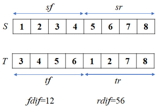
Figure 5.
Setup in LS8.
< setup >
Definition 4.
In the address of node S, there is a set sf = {S1S2S3 … Sn/2}, and sr = {Sn/2+1, … Sn}. In the case of node T, tf = {t1t2t3 … tn/2}, and tr = {tn/2+1, … tn}.
Definition 5.
Set fdif = {sf} − {tf}, and set rdif = {sr} − {tr}. In fdif and rdif, there is a sequential order, and the mth rdif element is denoted by rdif[m].
In Figure 5, for example, suppose S = 12345678 and T = 34561278. Then sf = {1, 2, 3, 4}, tf = {3, 4, 5, 6}, sr = {5, 6, 7, 8}, and tr = {1, 2, 7, 8}. In this case, fdif = {1, 2}, rdif = {5, 6}, |fdif| = |rdif| = 2, rdif[1] = 5, and rdif[2] = 6.
Routing is performed recursively using a typical separate-and-conquer method. Because it has already been conquered in the separation process, there is no additional conquer work to be performed when the separation is completed. The separation() of Algorithm 2 divides the symbols into two regions: separation() exchanges fdif in sf with rdif in sr. Once separation() is executed, there is no additional symbol movement between sf and sr. Separation() is then executed again on sf and sr. If |sf| = |sr| = 1, the separation() is terminated, and the routing is complete.
We provide an example to clarify the routing process. This explanation should be read with reference to Figure 6 and the routing algorithm. In LS8, let S = 32861457 and T = 12345678. fdif = {sf} − {tf} = {8, 6}, and rdif = {sr} − {tr} = {1, 4}. |fdif| = |rdif| = 2. Because |fdif| is not greater than 2 (= n/4), swap ① in the routing algorithm is skipped. In separation(), symbols 8 and 6 in sf and symbols 1 and 4 in sr are exchanged with each other. Figure 6 shows the stages in which the separation() is executed. In stage 1, sf = {4, 1, 3, 2}, and sr = {6, 8, 5, 7}. In stage 2, the same operation is repeated at sf and sr. Thus, S = sf = {4, 1, 3, 2} and T = tf = {1, 2, 3, 4}, and 4 in sf and 2 in sr are exchanged. As a result, sf = {2, 1} and sr = {4, 3}. In the next stage, the results are sf = {1, 2} and sr = {3, 4}. The operations are the same in the remaining part. If the skipped part is included, the entire routing path is as follows:
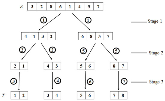
Figure 6.
Separation() call steps and sequence in LS8.
The first execution of separation():
The second execution of separation():
The third execution of separation():
The fourth execution of separation():
S = 32861457 → SE2 → 86321457 → SE4 → 14578632 → EE5 → 84571632 → SE1 → 48571632 → SE4 → 16324857 → SE1 → 61324857 → EE5 → 41326857.
41326857 → SE2 → 32416857 → SE1 → 23416857 → EE3 → 43216857 → SE2 → 21436857.
21436857 → SE1 → 12436857.
12436857 → SE2 → 43126857 → SE1 → 34126857 → SE2 → 12346857.
The operations on sr are performed in the same way as those on sf, whereby 6857 becomes 5678. The processing sequence is illustrated in Figure 6.
The routing algorithm is shown in Algorithm 1, where = = is an equality operator and = is an assignment operation:
| Algorithm 1. routing(S, T) { |
| 1: if (|S| = =1) return end-if |
| 2: <set up > |
| 3: if (|fdif| > n/4) |
| 4: S = S → SEn/2 ----------------- swap ① |
| 5: <set up > |
| 6: end-if |
| 7: separation(S) |
| 8: routing(sf, tf) |
| 9: S = S → SEn/2 |
| 10: routing(sf, tr) |
| 11: S = S → SEn/2 |
| 12: } |
| Algorithm 2. separation(S) { |
| 1: for (m = 1; m ≤ |fdif|; m + +) { |
| 2: movemsb(sf, fdif[m]) |
| 3: SE n/2 |
| 4: movemsb(sf, rfdif[m]) |
| 5: SE n/2 |
| 6: } |
| 7: if (|fdif| is odd) SE n/2 end-if |
| 8: } |
The separation() exchanges symbols. The exchange method is as follows:
- The first symbol to be exchanged is moved to the MSB through the movemsb() function of Algorithm 3;
- A half is swapped through SEn/2;
- The second symbol to be exchanged is moved to the MSB through movemsb();
- MSB and S(n/2)+1 are exchanged with each other through EEn/2.
| Algorithm 3. movemsb(S, sm) { |
| 1: if (|S| == 1) return end-if |
| 2: h = the index of sm in S |
| 3: if |S|/2 < h SE n/2 end-if |
| 4: movemsb(sf, sm) |
| 5: } |
The diameter is an important measure for evaluating a graph. It is the farthest distance between two nodes in the graph when taking the shortest path. In the worst case, it is the routing path length, which represents the software cost when the graph is implemented as a system.
Theorem 6.
The diameter of LSn is 0.5n(log2n)2 + 0.75nlog2n.
Proof.
and
The diameter analysis can be replaced by an analysis of the worst-case time complexity of the routing algorithm. In Figure 6, because the size of the problem decreases by half after each iteration and the process ends when the size reaches 1, the number of stages is a = log2n. In the worst case, the number of symbols to be exchanged in a single stage is b = n/2. The operations required to exchange two symbols are movemsb(), SEn/2, movemsb(), and EEn/2. When the number of symbols to be exchanged is odd, the EE edge is only required once. In the worst case, movemsb() is required to be log2n for each symbol. The number of operations required to exchange the two symbols is therefore c = 2log2n + 2+1. Then, the following would be true:
Diameter k = number of stages a × internal time complexity of the stage,
Internal time complexity of a stage = (number of symbols to be exchanged b × number of operations required to exchange two symbols c)/2.
Thus,
□
diameter k = a × (bc)/2
= log2n × ((n/2 × (2log2n + 3))/2)
= log2n × n/4(2log2n + 3)
= log2n × (0.5nlog2n + 0.75n) = 0.5n(log2n)2 + 0.75nlog2n.
= log2n × ((n/2 × (2log2n + 3))/2)
= log2n × n/4(2log2n + 3)
= log2n × (0.5nlog2n + 0.75n) = 0.5n(log2n)2 + 0.75nlog2n.
Network cost is an important measure for the evaluation of a network. Table 1 lists the network cost of LSn versus various star graph-like networks. To calculate the network cost of other networks, we investigated the diameter and degree of stars [9], hyper stars [10], macro stars [11], matrix stars [12], bubble sort [13], and hierarchical stars [14]. The network cost is shown in O notation.

Table 1.
Network cost comparison of LSn with other star graph-like networks.
Since O(n(log2n)3) < O(n2), LS is superior to other star graph-like networks in terms of its network cost (Table 1).
5. Discussion
Countless graphs have been published in various fields. Graphs are designed based on the characteristics of the problem to be solved, which also determine the most suitable evaluation measures for a graph. General-purpose evaluation measures that can be used in numerous fields include symmetry and network cost. In this study, we investigated the network cost of the representative star graph-like networks that were published to date and proposed a symmetric log star graph with a low network cost. For the log star LSn, the number of nodes is n, the degree is 2log2n − 1, and the diameter is 0.5n(log2n)2 + 0.75nlog2n. The network cost of LSn is O(n(log2n)3), which is smaller than O(n2)—the network cost of star graph-like networks. We analyzed the topological properties, connectedness, symmetry, and subgraph properties of the LS and proposed a routing algorithm. It is expected that in the future, various algorithms, such as broadcasting, processor allocation, parallel path, Hamiltonian path, spanning tree, and embedding, will be studied with respect to this graph.
Author Contributions
Conceptualization, J.-H.S. and H.-O.L.; methodology, J.-H.S.; software, J.-H.S.; validation, J.-H.S.; formal analysis, J.-H.S.; investigation, J.-H.S.; resources, J.-H.S.; data curation, J.-H.S.; writing—original draft preparation, J.-H.S.; writing—review and editing, J.-H.S.; visualization, J.-H.S.; supervision, H.-O.L.; project administration, H.-O.L.; funding acquisition, H.-O.L. All authors have read and agreed to the published version of the manuscript.
Funding
This research was funded by the National Research Foundation of Korea (NRF) grant funded by the Korean government (MSIT) (No. 2020R1A2C1012363).
Conflicts of Interest
The authors declare no conflict of interest.
References
- Seo, J.; Kim, J.; Chang, H.J.; Lee, H. The hierarchical Petersen network: A new interconnection network with fixed degree. J. Supercomput. 2018, 74, 1636–1654. [Google Scholar] [CrossRef]
- Gross, J.L.; Yellen, J. Graph Theory and Its Applications, 2nd ed.; CRC Press: Boca Raton, FL, USA, 2005; pp. 417–468. [Google Scholar]
- Xu, Z.; Huang, X.; Jimenez, F.; Deng, Y. A new record of graph enumeration enabled by parallel processing. Math 2019, 7, 1214. [Google Scholar] [CrossRef]
- Ganesan, A. Cayley graphs and symmetric interconnection networks. arXiv 2017, arXiv:1703.08109. [Google Scholar]
- Bermond, J.-C.; Delorme, C.; Quisquater, J.-J. Strategies for interconnection networks: Some methods from graph theory. J. Parallel Distrib. Comput. 1986, 3, 433–449. [Google Scholar] [CrossRef]
- Akers, S.B.; Krishnamurthy, B. A group-theoretic model for symmertric interconnection network. IEEE Trans. Comput. 1989, 38, 555–565. [Google Scholar] [CrossRef]
- Lakshmivarahan, S.; Jwo, J.-S.; Dhall, S.K. Symmetry in interconnection networks based on Cayley graphs of permutation groups: A survey. Parallel Comput. 1993, 19, 361–407. [Google Scholar] [CrossRef]
- Li, J.J.; Ling, B. Symmetric graphs and interconnection networks. Future Gener. Comput. Syst. 2018, 83, 461–467. [Google Scholar] [CrossRef]
- Akers, S.B.; Harel, D.; Krishnamurthy, B. The Star Graph: An Attractive Alternative to the N-Cube. In Proceedings of the International Conference on Parallel Processing, Penn State University, University Park, PA, USA, 17–21 August 1987; The Pennsylvania State University Press: University Park, PA, USA, 1987; pp. 393–400. [Google Scholar]
- Bell, M.G.H. Hyperstar: A multi-path Astar algorithm for risk averse vehicle navigation. Transp. Res. Part B Methodol. 2009, 43, 97–107. [Google Scholar] [CrossRef]
- Yeh, C.H.; Varvarigos, E. Macro-Star Networks: Efficient Low-Degree Alternatives to Star Graphs for Large-Scale Parallel Architectures. In Proceedings of the Frontiers96 the Sixth Symposium on the Frontiers of Massively Parallel Computation, Annapolis, MD, USA, 27–31 October 1996; IEEE Computer Society Press: Los Alamitos, CA, USA, 1996. [Google Scholar]
- Lee, H.O.; Kim, J.S.; Park, K.W.; Seo, J.H. Matrix Star Graphs: A New Interconnection Network Based on Matrix Operations. In Proceedings of the ACSAC: Asia-Pacific Conference on Advances in Computer Systems Architecture, Singapore, 24–26 October 2005; Srikanthan, T., Xue, J., Chang, C.H., Eds.; Springer: Berlin/Heidelberg, Germany, 2005; Volume 3740, pp. 478–487. [Google Scholar]
- Wang, S.; Yang, Y. Fault tolerance in bubble-sort graph networks. Theor. Comput. Sci. 2012, 421, 62–69. [Google Scholar] [CrossRef][Green Version]
- Song, Z.; Ma, G.; Song, D. Hierarchical Star: An optimal NoC Topology for High-performance SoC Design. In Proceedings of the 2008 International Multi-symposiums on Computer and Computational Sciences, Shanghai, China, 18–20 October 2008; IEEE: Piscataway, NJ, USA, 2008; pp. 158–163. [Google Scholar]
Publisher’s Note: MDPI stays neutral with regard to jurisdictional claims in published maps and institutional affiliations. |
© 2021 by the authors. Licensee MDPI, Basel, Switzerland. This article is an open access article distributed under the terms and conditions of the Creative Commons Attribution (CC BY) license (https://creativecommons.org/licenses/by/4.0/).