A Comparative Study of Image Descriptors in Recognizing Human Faces Supported by Distributed Platforms

Abstract

Face recognition is one of the emergent technologies that has been used in many applications. It is a process of labeling pictures, especially those with human faces. One of the critical applications of face recognition is security monitoring, where captured images are compared to thousands, or even millions, of stored images. The problem occurs when different types of noise manipulate the captured images. This paper contributes to the body of knowledge by proposing an innovative framework for face recognition based on various descriptors, including the following: Color and Edge Directivity Descriptor (CEDD), Fuzzy Color and Texture Histogram Descriptor (FCTH), Color Histogram, Color Layout, Edge Histogram, Gabor, Hashing CEDD, Joint Composite Descriptor (JCD), Joint Histogram, Luminance Layout, Opponent Histogram, Pyramid of Gradient Histograms Descriptor (PHOG), Tamura. The proposed framework considers image set indexing and retrieval phases with multi-feature descriptors. The examined dataset contains 23,707 images of different genders and ages, ranging from 1 to 116 years old. The framework is extensively examined with different image filters such as random noise, rotation, cropping, glow, inversion, and grayscale. The indexer’s performance is measured based on a distributed environment based on sample size and multiprocessors as well as multithreads. Moreover, image retrieval performance is measured using three criteria: rank, score, and accuracy. The implemented framework was able to recognize the manipulated images using different descriptors with a high accuracy rate. The proposed innovative framework proves that image descriptors could be efficient in face recognition even with noise added to the images based on the outcomes. The concluded results are as follows: (a) the Edge Histogram could be best used with glow, gray, and inverted images; (b) the FCTH, Color Histogram, Color Layout, and Joint Histogram could be best used with cropped images; and (c) the CEDD could be best used with random noise and rotated images.

1. Introduction

Face recognition is a new technology that has been recently introduced. It has been used and implemented in many fields, such as video surveillance, human–machine interaction, virtual reality, and law enforcement [1]. It can be viewed as a Visual Information Retrieval (VIR) concept which has existed for many years. In addition, VIR is defined by Li et al. in [2] as the research area that attempts to provide means of organization, indexing, annotation, and retrieval of visual information from unstructured big data sources. Its goal is to match and rank the retrieved images by their relevance to a given query. This paper is inspired by the VIR concept, but this work concerns human face recognition. However, the proposed framework is more generic, involving many other applications.

Many studies in the face recognition field focus on testing feature extraction descriptors on various datasets other than human faces such as landscapes, animals, etc. Few efforts have been devoted to exploring the existing feature extraction descriptors with human face datasets. The difficulties come from the similarity of the faces and the small differences in human faces, as well as inaccurate capturing positions and noise. In addition, previous research focuses on separate descriptors for specific applications.

This paper’s research contribution is to develop a face recognition testing and validation innovative framework to determine the optimal feature extraction descriptors to be used in the human face recognition process. It also analyzes and evaluates different descriptors based on a rich face recognition library [3] with 23,707 images of different genders and ages, ranging from 1 to 116 years old. Moreover, the proposed framework utilizes the concept of distributed indexing and retrieval for the benefit of large-scale image retrieval applications. Furthermore, it compares the used feature extraction descriptors in terms of (a) elapsed time, (b) accuracy, (c) retrieval rank, and (d) retrieval score. Our findings and recommendations are concluded at the end of our extensive experimentation, where we identify the importance of specific descriptors to certain cases. The proposed innovative framework proves that image descriptors could be efficient in face recognition even with noise added to the images based on the outcomes.

Due to the many abbreviations used in this paper, Table 1 summarizes all of the used acronyms for ease of reading.

Table 1. List of acronyms.

Abbreviation	Meaning
CEDD	Color and Edge Directivity Descriptor
FCTH	Fuzzy Color and Texture Histogram Descriptor
JCD	Joint Composite Descriptor
PHOG	Pyramid of Gradient Histograms Descriptor
CLD	Color Layout Descriptor
JCD	Joint Composite Descriptor
CCDs	Compact Composite Descriptors
SVM	Support Vector Machines
CEDD	Hashed Color and Edge Directivity Descriptor
VIR	Visual Information Retrieval
3D	Three Dimension
PCA	Principal Component Analysis
DCT	Discrete Cosine Transform
LDA	Linear Discriminant Analysis
ICA	Independent Component Analysis
LBP	Local Binary Pattern
EBGM	Elastic Base Graph Method
LBP	Local Binary Pattern
FERET	Facial Recognition Technology
LFW	Labeled Faces in the Wild
JAFFE	Japanese Female Facial Expression
CBIR	Content-Based Image Retrieval
LMP	Local Multiple Patterns
MB-LMP	Multi-Scale Block LMP
DI	Distributed Indexer
CCTV	Closed-Circuit Television
EM	Commonly Electromagnetic
RGB	Red, Green, Blue
HSV	Hue, Saturation, Value
HMMD	Hue-Max-Min-Diff
MPEG-7	Multimedia Content Description Interface
Diff	Difference
Sum	Summation
SIFT	Scale Invariant Feature Transform
SURF	Speeded-Up Robust Features
MSER	Maximally Stable Extremal Regions
BRIEF	ORB (Oriented Fast and Rotated Brief)
BRISK	Binary Robust Invariant Scalable Key Points
FREAK	Fast Retina Key Point
HSL	Hue, Saturation, Lightness

This research will first highlight related studies conducted in this field in Section 1. Section 2 illustrates the proposed face recognition framework used for conducting this research. Then, the presentation and discussion of the results are described in Section 3. Finally, highlights of the most significant findings and future work are provided in the conclusion section.

2. Literature Review

2.1. Face Recognition

Face recognition has become a very active area of research since the 1970s [1] due to its wide range of applications in many fields such as public security, human–computer interaction, computer vision, and verification [2,4]. Face recognition systems could be applied in many applications such as (a) security, (b) surveillance, (c) general identity verification, (d) criminal justice systems, (e) image database investigations, (f) “Smart Card” applications, (g) multi-media environments with adaptive human–computer interfaces, (h) video indexing, and (i) witness face reconstruction [5]. However, there are major drawbacks or concerns for face recognition systems including privacy violation. Moreover, Wei et al. [6] discussed some of the facial geometric features such as eye distance to the midline, horizontal eye-level deviation, eye–mouth angle, vertical midline deviation, ear–nose angle, mouth angle, eye–mouth diagonal, and the Laplacian coordinates of facial landmarks. The authors claimed that these features are comparable to those extracted from a set with much denser facial landmarks. Additionally, Gabryel and Damaševičius [7] discussed the concept of keypoint features where they adopted a Bag-of-Words algorithm for image classification. The authors based their image classification on the keypoints retrieved by the Speeded-Up Robust Features (SURF) algorithm.

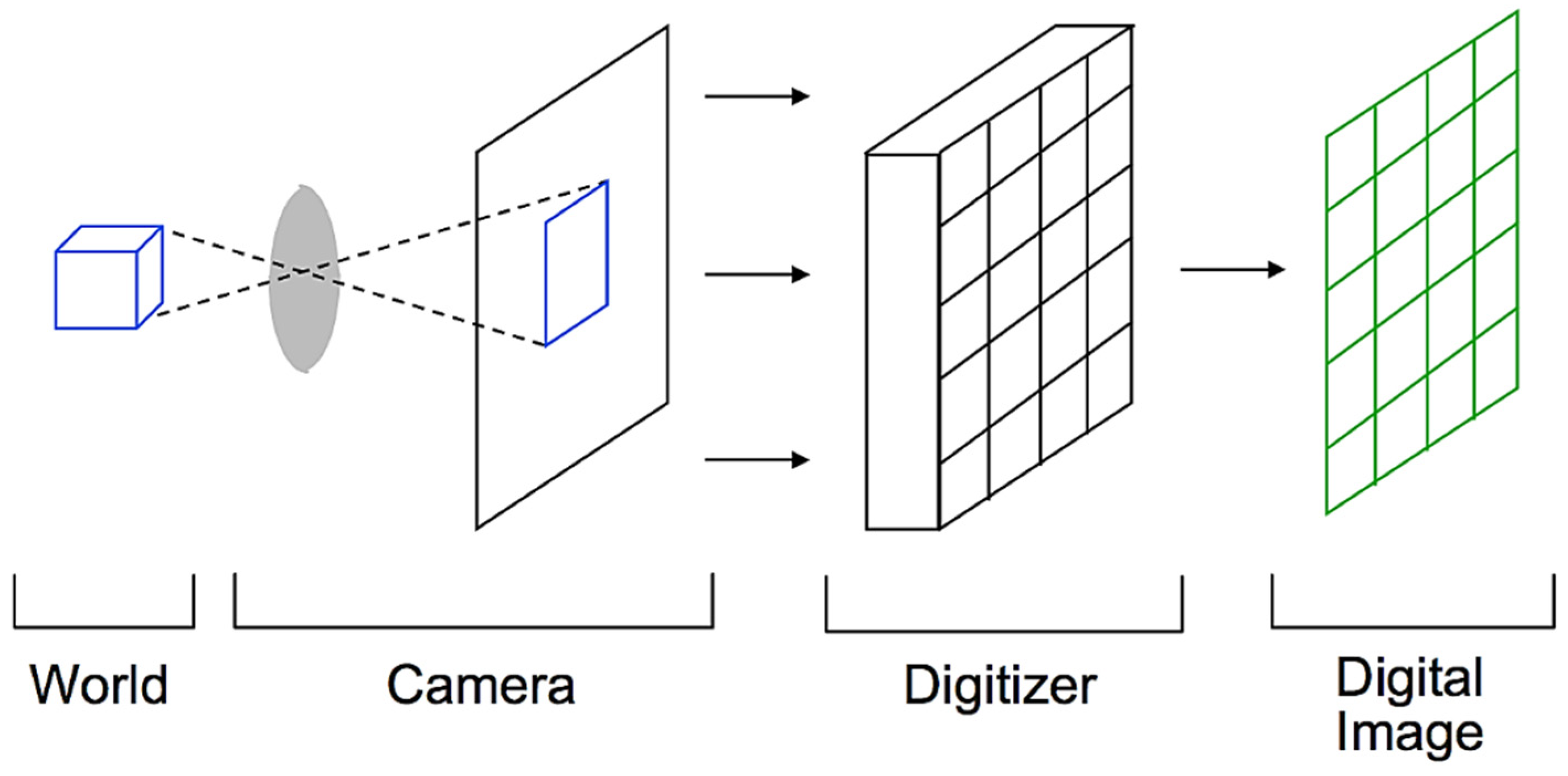
This is considered one of the most challenging zones in the computer vision field. The facial recognition system is a technology that can identify or verify an individual from an acquisition source, e.g., a digital image or a video frame. The first step for face recognition is face detection, which means localizing and extracting areas of a human’s face from the background. In this step, active contour models are used to detect edges and boundaries of the face. Recognition in computer vision takes the form of face detection, face localization, face tracking, face orientation extraction, facial features, and facial expressions. Face recognition needs to consider some technical issues, e.g., poses, occlusions, and illumination [8].

There are many methods for facial recognition systems’ mechanism; generally, they compare selected or global features of a specified face image with a dataset containing many images of faces. These extracted features are selected based on examining patterns of individuals’ facial color, textures, or shape. The human face is not unique. Hence, several factors cause variations in facial appearance. The facial appearance variations develop two image categories, which are intrinsic and extrinsic factors [5].

Emergent face recognition systems [9] have achieved an identification rate of better than 90% for massive databases within optimal poses and lighting conditions. They have moved from computer-based applications to being used in various mobile platforms such as human–computer interaction with robotics, automatic indexing of images, surveillance, etc. They are also used in security systems for access control in comparison with other biometrics such as eye iris or fingerprint recognition systems. Although the accuracy of face recognition systems is less accurate than other biometrics recognition systems, they has been adopted extensively because of their non-invasive and contactless processes.

The face recognition process [10,11,12] starts with a face detection process to isolate a human face within an input image that contains a human face. Then, the detected face is pre-processed to obtain a low-dimensional representation. This low-dimensional representation is vital for effective classification. Most of the issues in recognizing human faces arise because they are not a rigid object, and the image can be taken from different viewpoints. It is important for face recognition systems to be resilient to intrapersonal variations in an image, e.g., age, expressions, and style, but still able to distinguish between different people’s interpersonal image variations [13].

According to Schwartz et al. [14], the face recognition method consists of (a) detection: detecting a person face within an image; (b) identification: an unknown person’s image is matched to a gallery of known people; and (c) verification: acceptance or denial of an identity claimed by a person. Previous studies stated that applying face recognition in well-controlled acquisition conditions gives a high recognition rate even with the use of large image sets. However, the face recognition rate became low when applying it in uncontrolled conditions, leading to a more laborious recognition process [14].

The following is the chronological summary of some of the relevant studies conducted in the area of face recognition.

In 2012, Rouhi et al. [15] reviewed four techniques for face recognition in the feature extraction phase. The four techniques are 15-Gabor filter, 10-Gabor filter, Optimal- Elastic Base Graph Method (EBGM), and Local Binary Pattern (LBP). They concluded that the weighted LBP has the highest recognition rate, whereas the non-weighted LBP has the maximum performance in the feature extraction between the used techniques. However, the extracted recognition rates in the 10-Gabor and 15-Gabor filter techniques are higher than those in the EBGM and Optimal-EBGM methods, even though the vector length is long. In [6], Schwartz et al. used a large and rich set of facial identification feature descriptors using partial squares for multichannel weighting. They then extend the method to a tree-based discriminative structure to reduce the time needed to evaluate samples. Their study shows that the proposed identification method outperforms current state-of-the-art results, particularly in identifying faces acquired across varying conditions.

Nanni et al. [16] conducted a study to determine how best to describe a given texture using a Local Binary Pattern (LBP) approach. They performed several empirical experiments on some benchmark databases to decide on the best feature extraction method using LBP-based techniques. In 2014, Kumar et al. [17] completed a comparative study to compare global and local feature descriptors. This study considered experimental and theoretical aspects to check those descriptors’ efficiency and effectiveness. In 2017, Soltanpour et al. [18] conducted a survey illustrating a state-of-the-art for 3D face recognition using local features, with the primary focus on the process of feature extraction. Nanni et al. [16] also presented a novel face recognition system to identify faces based on various descriptors using different preprocessing techniques. Two datasets demonstrate their approach: (a) the Facial Recognition Technology (FERET) dataset and (b) the Wild Faces (LFW) dataset. They use angle distance in FERET datasets, where identification was intended. In 2018, Khanday et al. [19] reviewed various face recognition algorithms based on local feature extraction methods, hybrid methods, and dimensionality reduction approaches. They aimed to study the main methods/techniques used in recognition of faces. They provide a critical review of face recognition techniques with a description of major face recognition algorithms.

In 2019, VenkateswarLal et al. [20] suggested that an ensemble-aided facial recognition framework performed well in wild environments using preprocessing approaches and an ensemble of feature descriptors. A combination of texture and color descriptors is extracted from preprocessed facial images and classified using the Support Vector Machines (SVM) algorithm. The framework is evaluated using two databases, the FERET dataset samples and Labeled Faces in the Wild dataset. The results show that the proposed approach achieved a good classification accuracy, and the combination of preprocessing techniques achieved an average classification accuracy for both datasets at 99% and 94%, respectively. Wang et al. [21] proposed a multiple Gabor feature-based facial expression recognition algorithm. They evaluated the effectiveness of their proposed algorithm on the Japanese Female Facial Expression (JAFFE) database, where the algorithm performance primarily relies on the final combination strategy and the scale and orientation of the features selected. The results indicate that the fusion methods perform better than the original Gabor method. However, the neural network-based fusion method performs the best.

Latif et al. [22] presented a comprehensive review of recent Content-Based Image Retrieval (CBIR) and image representation developments. They studied the main aspects of image retrieval and representation from low-level object extraction to modern semantic deep-learning approaches. Their object representation description is achieved utilizing low-level visual features such as color, texture, spatial structure, and form. Due to the diversity of image datasets, single-feature representation is not possible. There are some solutions to be used to increase CBIR and image representation performance, such as the utilization of low-level feature infusion. The conceptual difference could be minimized by using the fusion of different local features as they reflect the image in a patch shape. It is also possible to combine local and global features. Furthermore, traditional machine learning approaches for CBIR and image representation have shown good results in various domains. Recently, CBIR research and development have shifted towards utilizing deep neural networks that have presented significant results in many datasets and outperformed handcrafted features prior to fine-tuning of the deep neural network.

In 2020, Yang et al. [23] developed a Local Multiple Pattern (LMP) feature descriptor based on Weber’s extraction and face recognition law. They modified Weber’s ratio to contain change direction to quantize multiple intervals and to generate multiple feature maps to describe different changes. Then LMP focuses on the histograms of the non-overlapping regions of the feature maps for image representation. Further, a multi-scale block LMP (MB-LMP) is presented to generate more discriminative and robust visual features because LMP could only capture small-scale structures. This combined MB-LMP approach could capture both the large-scale and small-scale structures. They claimed that the MB-LMP is computationally efficient using an integral image. Their LMP and MB-LMP are evaluated upon four public face recognition datasets. The results demonstrate that there is a promising future for the proposed LMP and MB-LMP descriptors with good efficiency.

2.2. Face recognition Acquisition and Processing Techniques

Research and development in the face recognition has significantly progressed over the last few years. The following paragraphs briefly summarize some of used face recognition techniques.

Traditional approach: This approach uses algorithms to identify facial features by extracting landmarks from an individual’s face image. The first type of algorithms would analyze the size and/or shape of the eyes’ relative position, nose, cheekbones, mouth, and jaw. The output is used to match the selected image with similar features within an image set. On the other hand, some algorithms adopt template matching techniques, and it is conducted via analyzing and compressing only face data that are important for the face recognition process and then compare it with a set of face images.

Dimensional recognition approach: This approach utilizes 3D sensors to capture information of an individual’s face shape [13,18]. These sensors work by projecting structured light on an individual’s face and work as a group with each other to capture different views of the face. The information is used to identify unique and distinctive facial features such as the eye socket contour, chin, and nose. This approach overcomes the traditional approach by identifying faces from different angles, and it is not affected by light changes.

Texture analysis Approach: The texture analysis approach, also known as Skin Texture Analysis [4], utilizes the visual details of the skin of an individual’s face image. This transforms the distinctive lines, patterns, and spots in the skin of a person into numerical value. A skin patch of an image is called a skinprint. This patch is broken up into smaller blocks, and then the algorithms transform/convert them into measurable and mathematical values for the system to be able to identify the actual skin texture and any pores or lines. This allows identifying the contrast between identical pairs that could not possibly be carried out by traditional face recognition tools alone. The test result of this approach showed that it could increase the performance of face recognition by 20–25%.

Thermal camera approach: This approach requires a thermal camera as a technology for face image acquisition. It produces different forms of data for an individual’s face by detecting only the head shape and ignoring other accessories such as glasses or hats [18]. Compared to traditional image acquisition, this approach can capture face image at night or even in a low-light condition without an external source of light, e.g., flash. One major limitation of this approach is that the dataset of such thermal images is limited for face recognition in comparison to other types of datasets.

Statistical approach: There are several statistical techniques for face recognition, e.g., Principal Component Analysis (PCA) [13], Eigenfaces [24], and Fisherfaces [25]. The methods in this approach can be mainly categorized into:

-

Principal Component Analysis (PCA): this analyzes data to identify patterns and find patterns reducing the dataset’s computational complexity with nominal loss of information.

-

Discrete Cosine Transform (DCT): this is used for local and global features to identify the related face picture from a database [26].

-

Linear Discriminant Analysis (LDA): this is a dimensionality reduction technique that is used to maximize the class scattering matrix measure.

-

Independent Component Analysis (ICA): this decreases the second-order and higher-order dependencies in the input and determines a set of statistically independent variables [27].

Hybrid approach: Most of the current face recognition systems have combined different approaches from the list mentioned above [15]. Those systems would have a higher accuracy rate when recognizing an individual’s face. This is because, in most cases, the disadvantages of one approach could be overcome by another approach. However, this cannot be generalized.

There are several software and tools used in image retrieval, and the most well-known ones are MATLAB [28], OpenCV [29], and LIRE [30]. The LIRE Library is the tool we utilized in this paper. A Java tool is developed for the purpose of framework implementation.

2.3. Image Descriptors Analysis

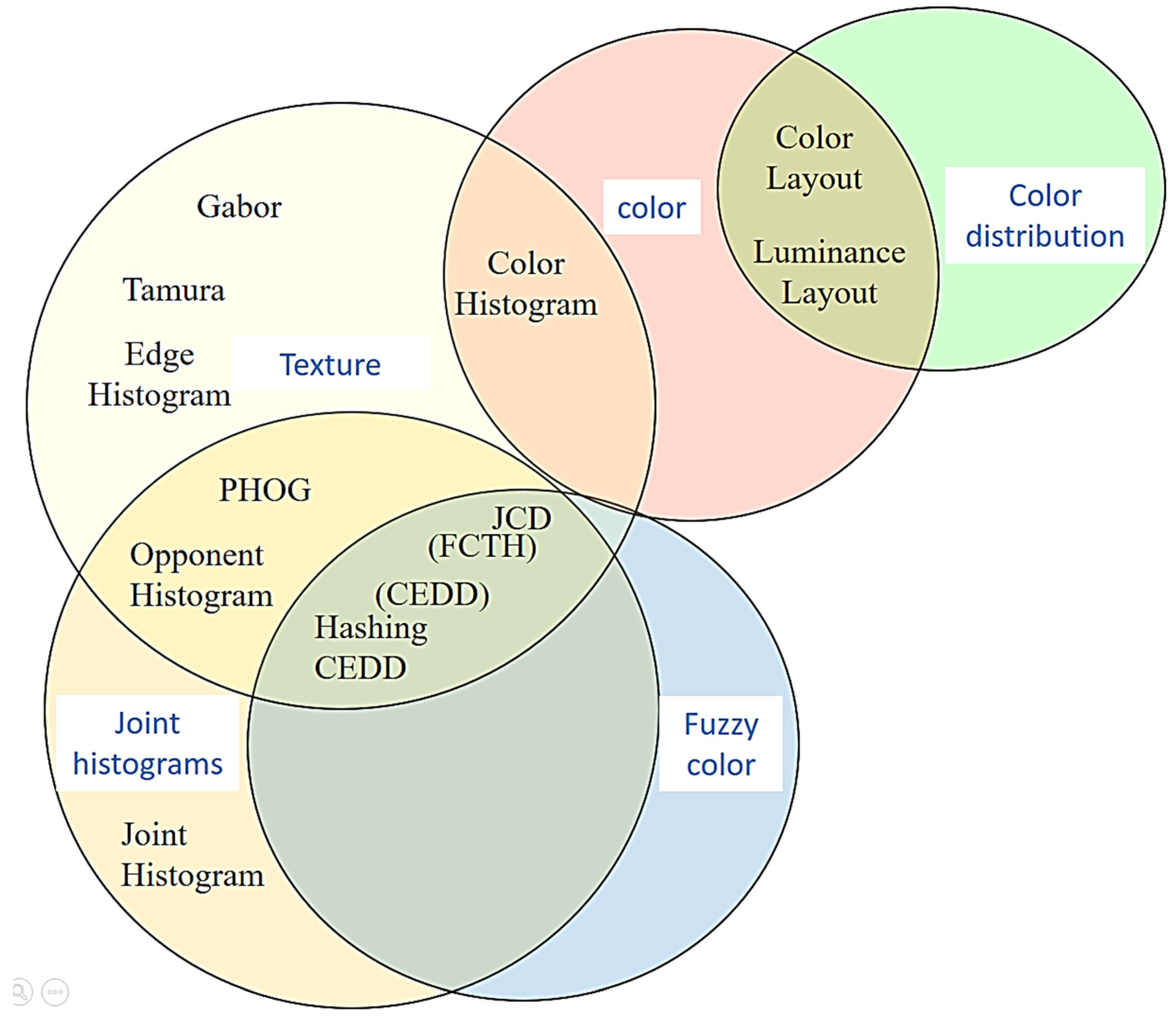
The following Figure 1 shows most of the image descriptors stated in the literature [17]. The inner-circle represents the type of descriptors, while the middle circle represents the different descriptors. Moreover, the outer circle represents the features used by each descriptor. However, this paper experiments with different features on a dataset of faces, and specific descriptors that cover most of the previously mentioned features are selected. The selected descriptors are briefly described in the following paragraphs:

Figure 1. Common descriptors stated in the literature.

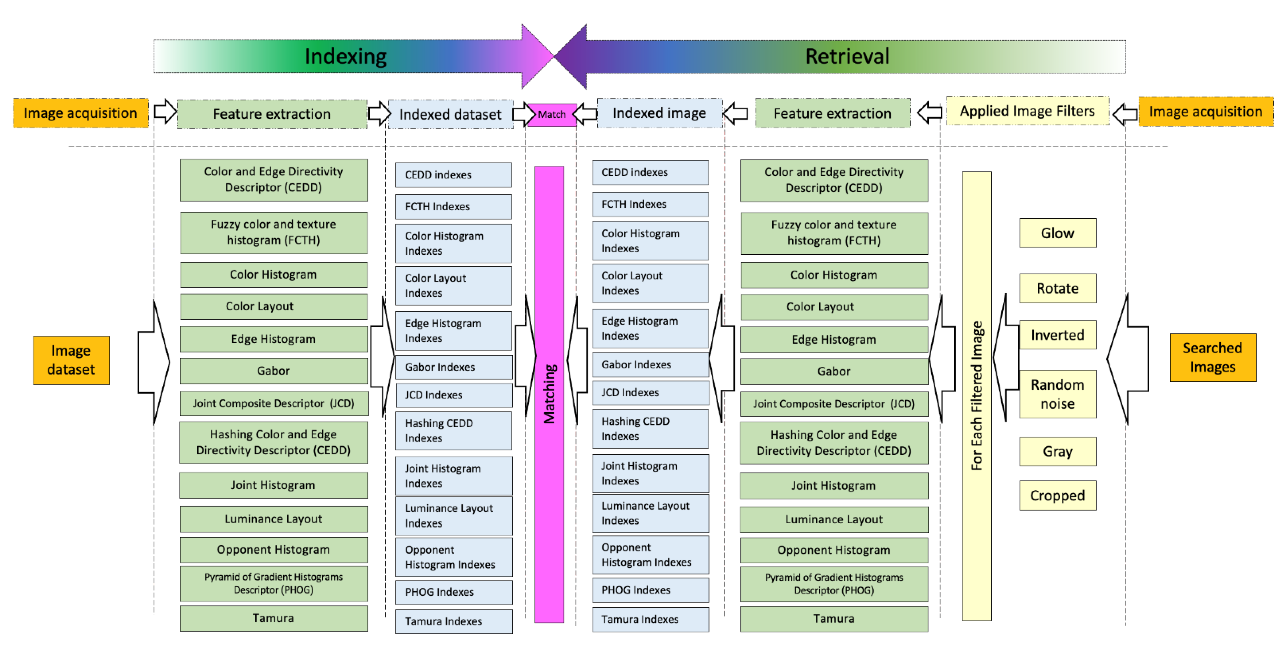
Color and Edge Directivity Descriptor (CEDD): The CEDD incorporates fuzzy information about color and edge. This blends a black, brown, white, dark red, red, light red, medium orange, light orange, dark purple, yellow, light yellow, dark green, dark green, dark cyan, cyan, light cyan, dark blue, blue, light blue, dark magenta, magenta, and light magenta with six different colors. It is a low-level image extraction function that can be used for indexing and retrieval. This integrates details about color and texture in a histogram. The size of the CEDD is limited to 54 bytes per image, making it ideal for use in large image databases. One of the CEDD’s most important attributes is the low computing power needed to extract it, relative to most MPEG-7 descriptors’ specifications.

Fuzzy Color and Texture Histogram (FCTH) Descriptor [31]: The FCTH descriptor uses the same fluffy color scheme used by CEDD, but it uses a more detailed edge definition with 8 bins, resulting in a 192-bin overall function.

Luminance Layout Descriptor [32]: The luminance of light is a unit intensity value per light area of the movement in a given direction. The luminance of light may take the same light energy and absorb it at a time or disperse it across a wider area. Luminance is, in other words, a light calculation not over time (such as brightness) but over an area. The luminance can be displayed as L in Hue, Saturation, Lightness (HSL) in photo editing. The layer mask is based on a small dark or light spectrum in the picture. It helps one explicitly alter certain parts, such as making them lighter or darker or even changing their color or saturation.

Color Histogram Descriptor [33]: This descriptor is one of the most intuitive and growing visual descriptors. Each bin in a color histogram reflects the relative pixel quantity of a certain color. One color bin is assigned to each pixel of an image, and the corresponding count increases. Intuitively, a 16M color image will result in a 16M bins histogram. Usually, the color data are quantized to limit the number of measurements; thus, identical colors are treated in the original color space as if they were the same, and their rate of occurrence is measured for the same bin. Color quantization is a crucial step in building a characteristic. The most straightforward approach to color quantization is to divide the color space of the Red, Green, Blue (RGB) into partitions of equal size, similar to stacked boxes in 3D space.

Color Layout Descriptor [33]: A Color Layout Descriptor (CLD) is designed to capture a picture’s spatial color distribution. The function’s extraction process consists of two parts: grid-based representative color selection and the quantization of discrete cosine transform. Color is the visual content’s most basic value; thus, colors can be used to define and reflect an object. The Multimedia Content Description Interface (MPEG-7) specification is tested as the most effective way to describe the color and chose those that produced more satisfactory results. The norm suggests different methods of obtaining such descriptors, and one tool for describing the color is the CLD, which enables the color relationship to be represented.

Edge Histogram Descriptor [34]: The Edge Histogram function is part of the standard MPEG-7, a multimedia meta-data specification that includes many visual information retrieval features. The function of the Edge Histogram captures the spatial distribution within an image of (undirected) edges. Next, the image is divided into 16 blocks of equal size, which are not overlapping. The data are then processed for each block edge and positioned in a 5-bin histogram counting edge in the following categories: vertical, horizontal, 35mm, 135 mm, and non-directional. This function is mostly robust against scaling.

Joint Composite Descriptor (JCD) Descriptor [35]: The JCD is a mixture of the CEDD and FCTH. Compact Composite Descriptors (CCDs) are low-level features that can be used to describe different forms of multimedia data as global or local descriptors. SIMPLE Descriptors are the regional edition of the CCDs. JCD consists of seven areas of texture, each of which consists of 24 sub-regions corresponding to color areas. The surface areas are as follows: linear region, horizontal activation, 45-degree activation, vertical activation, 135-degree activation, horizontal and vertical activation, and non-directional activation.

Joint Histogram Descriptor [35]: A color histogram is a vector where each entry records the number of pixels in the image. Before histogramming, all images are scaled to have the same number of pixels; then, the image colors are mapped into a separate color space with n colors. Usually, images are represented in the color space of the RGB using some of the most important bits per color channel to isolate the space. Color histograms do not relate spatial information to certain color pixels; they are primarily invariant in image reference rotation and translation. Therefore, color histograms are resistant to occlusion and lens perspective changes.

Opponent Histogram Descriptor [36]: The opposing histogram is a mixture of three 1D histograms based on the opponent’s color space streams. The frequency is displayed in channel O3, Equation (1), and the color data are displayed in channels O1 and O2. The offsets will be cancelled if they are equal for all sources (e.g., a white light source) due to the subtraction in O1 and O2. Therefore, in terms of light intensity, these color models are shift invariant. There are no invariance properties in the frequency stream O3. The competing color space histogram intervals have ranges that are different from the RGB standard.

$$\left(\begin{array}{c}O1\\ O2\\ O3\end{array}\right)= \left(\begin{array}{c}\frac{R-G}{\sqrt{2}}\\ \frac{R+G-2B}{\sqrt{6}}\\ \frac{R+G+B}{\sqrt{3}}\end{array}\right)$$

(1)

Pyramid of Gradient Histograms (PHOG) Descriptor [37]: The PHOG descriptor is used to apply material identification. Support Vector Machines (SVM) can use the kernel trick to perform an effective non-linear classification, mapping their inputs into high-dimensional feature spaces. PHOG is an outstanding global image shape descriptor, consisting of a histogram of the gradients of orientation over each image’s sub-region at each resolution point. PHOG is an outstanding global image form descriptor, consisting of a histogram of the gradients of orientation at each resolution level over each object sub-region.

Tamura Descriptor [38]: The features of Tamura represent texture on a global level; thus, they are limited in their utility for images with complex scenes involving different textures. The so-called Tamura features are the classic collection of basic features. Generally, six different surface characteristics are identified: (i) coarseness (coarse vs. fine), (ii) contrast (high contrast vs. low contrast), (iii) directionality (directional vs. non-directional), (iv) line-like vs. blob-like, (v) regularity (regular vs. irregular), and (vi) roughness (rough vs. smooth).

Gabor Descriptor [39]: A Gabor Descriptor named after Dennis Gabor. It is a linear filter used for texture analysis, meaning that it essentially analyzes whether there is any particular frequency material in the image in specific directions around the point area of analysis in a localized field. A 2D Gabor filter is a Gaussian kernel function that is modulated by a sinusoidal plane wave in the spatial domain.

Hashing CEDD Descriptor [40]: Hashed Color and Edge Directivity Descriptor (CEDD) is the main feature, and a hashing algorithm puts multiple hashes per image, which are to be translated into words. This makes it much faster in retrieval without losing too many images on the way, which means the method has an acceptable recall.

The following Table 2 summarizes the related work stated in this section.

Table 2. Summary of the related work.

Category	Paper ID	Description
Face recognition system	[9]	It is based on Emergent Face Recognition Systems. It has been used for mobile applications.
	[10,11,12]	It is based on face detection processes to isolate a human face within an input image that contains a human face.
	[14]	They proposed an approach that works based on three phases, which are detection, identification, and verification.
	[15]	This paper reviewed four different face recognition techniques and compared their results. The algorithms are 15-Gabor filter, 10-Gabor filter, Optimal-EBGM, and LBP.
	[16]	This paper studied how best to describe a given texture using a Local Binary Pattern (LBP) approach.
	[6]	This paper discussed some of the facial geometric features such as eye distance to the midline, horizontal eye-level deviation, eye–mouth angle, vertical midline deviation, ear–nose angle, mouth angle, eye–mouth diagonal, and Laplacian coordinates of facial landmarks.
	[7]	This paper adopted the Bag-of-Words algorithm for image classification.
	[17]	This paper presented a comparative study to compare global and local feature descriptors. This study considered experimental and theoretical aspects to check the descriptors’ efficiency and effectiveness.
	[18]	This paper forms a good reference for 3D face recognition using local features, with the primary focus on the process of feature extraction.
	[16]	This paper presented a face recognition system to identify faces based on various descriptors using different preprocessing techniques.
	[20]	This paper suggested an ensemble-aided facial recognition framework. A combination of texture and color descriptors is extracted from preprocessed facial images and classified using the SVM algorithm
	[22]	This paper presented a comprehensive review of recent CBIR and image representation developments.
	[23]	This paper developed a Local Multiple Pattern (LMP) feature descriptor based on Weber’s extraction and face recognition law. The authors modified Weber’s ratio to contain change direction to quantize multiple intervals and to generate multiple feature maps to describe different changes.
Face recognition acquisition and processing techniques	[13]	This paper provided an approach that utilizes 3D sensors to capture information of an individual’s face shape.
	[5]	This paper utilized a texture analysis approach, also known as skin texture analysis, that uses the visual details of the skin of an individual’s face image.
	[21]	This paper used a thermal camera as a technology for face image acquisition. It produced different forms of data for an individual’s face by detecting only the head shape and ignoring other accessories such as glasses or hats.
	[13,24] [25,27]	These papers utilized the statistical approach such as Principal Component Analysis (PCA), Eigenfaces, Fisherfaces, and Independent Component Analysis (ICA).
	[15]	This paper used a hybrid approach of the previously mentioned algorithms.
Descriptors	[31,32,33,34,35,36,37,38,39,40]	These papers summarized the list of image descriptors.

3. Proposed Face Recognition Framework

In this section, a description of the proposed framework for face recognition with different descriptors is provided. The framework consists of two main components, distributed indexer and distributed retrieval. As shown in Figure 2, the indexer comprises image acquisition, feature extraction, distributed processing, and indexed image storage blocks. On the other hand, the retrieval involves image acquisition, image filtering, parallel feature extraction, and assessment blocks.

Figure 2. The proposed framework for face recognition with different descriptors.

3.1. Distributed Indexer (DI)

The distributed indexer, in this context, refers to the processing of the images and prepares them for the retrieval phase. It utilizes different image features as well as new technology such as multicore processors, parallel processors, clusters, and Cloud technology. Therefore, the framework is open to be used on any of the distributed technologies. Throughout the following subsections the components of the distributed indexer (DI) are described.

3.2. Image Acquisition

Image acquisition is the development of a digitally encoded image of an object’s visual properties, such as a physical scene or an object’s internal structure. The image acquisition block is used to transfer images into an array of numerical data that a computer could handle. Image sources could be scanners, cameras, Closed-Circuit Television (CCTV), etc. Therefore, images come with different qualities based on the image source. Image Acquisition is the first step in any image processing system. As shown in Figure 3, image acquisition has three steps, including capturing the image using a camera, digitization, and the final step forming the digital image.

Figure 3. Image acquisition steps.

3.3. Feature Extraction

This component tries to involve the best of the image visual features, and it is open for any other image features. One of the important image features are visual features where they could be global or local; global features encode all of the image properties such as color and histogram, while local features focus on the crucial information in the image that might be used for generating image indexing [14,15]. Those features will be represented as an image descriptor, as will be described later in this section. Since this research’s main idea is not only detecting faces but also comparing them, the problem became more difficult with different image characteristics and embedded noises. Therefore, the extraction of image descriptors is considered a critical phase where such descriptors are later encoded in a feature vector. Descriptors have to be robust, compact, and representative. After all, a suitable metric is used to compute the distance between the two image vectors.

The first feature that can be extracted is the color. It is the most natural feature to be extracted from an image; simultaneously, it is easy to obtain, and it is invariant in image resizing and rotation. Two main steps are required to extract the color, which are selecting the color model and computing the descriptor. As it is mostly used in the literature, the color model or color space is the specification of the coordinate system where a point represents each color.

The most used color models are grayscale, RGB, HSV, and Hue-Max-Min-Diff (HMMD). A grayscale color model represents the image pixel intensity; the RGB color uses the three light colors (R, G, and B) that are normalized to the range [0, 1]. The RGB model has different variants, including the opponent color space. HSV (Hue, Saturation, Value) is the RGB color model’s alternate representations. Colors of each hue are arranged in these models in a radial slice, around a central axis with neutral colors varying from black on the bottom to white on the top. The HSV representation models the way the colors are blended, with the saturation dimension representing different tints of brightly colored paint and the quality dimension resembling the combination of those paints with varying amounts of black or white paint. Furthermore, the HMMD (Hue-Max-Min-Diff) color space is developed based on MPEG-7 visual descriptor standardization efforts where the Max, Min, Diff, and Sum are computed for the (R, G, and B) colors.

The second color feature to be extracted is the color histograms. The color histogram is one of the most common visual descriptors. It is a representation of the relative number of pixels with a particular color. The dominant color feature could be extracted from the histogram, representing the most color(s) found in the picture.

The third color feature to be extracted is the fuzzy color. The fuzzy color comes into the picture when some colors cannot be identified. Therefore, fuzzy colors can quantify the unidentified colors to their most similar colors.

Another important feature is related to texture features. Texture similarity is one of the essential features; for instance, similar spatial arrangements of colors (or gray levels) are not necessarily the same colors (or gray levels). Other texture features, such as Tamura features, describe texture on a global level and are also crucial in image comparison, such as:

-

Coarseness (coarse vs. fine),

-

Contrast (high contrast vs. low contrast),

-

Directionality (directional vs. non-directional),

-

Line-likeness (line-like vs. blob-like),

-

Regularity (regular vs. irregular),

-

Roughness (rough vs. smooth).

The Edge Histogram feature captures the spatial distribution of (undirected) edges within an image. This feature is mostly robust against scaling. There are some other local features related to interest points, corners, edges, or salient spots along with this feature.

One more important feature is the Frequency Domain Descriptors such as Scale Invariant Feature Transform (SIFT), SURF descriptor/detector, Maximally Stable Extremal Regions (MSER), ORB (Oriented Fast and Rotated Brief), BRIEF (Binary Robust Independent Elementary Features), BRISK (Binary Robust Invariant Scalable Key Points), and FREAK (Fast Retina Key Point). However, the most important features among the frequency domain descriptors are the Scale Invariant Feature Transform (SIFT) and the SURF descriptor/detector.

The descriptors used in this paper are summarized in Figure 4. As can be seen in Figure 4, the descriptors are categorized based on the existing features. One can notice that the Texture feature and Joint Histogram involve most of the descriptors. The joints in Figure 4 show the common image features between the descriptors. Therefore, these descriptors are carefully selected to represent all of the images’ features reported in the literature.

Figure 4. Categories of the used image descriptors.

3.4. Distributed Processing

This subsection is dedicated to the distributed processing block as part of the main framework. It has been learned from the image acquisition component that image processing may take a long time, and images might not come in a small number. For instance, in this paper, the processed images are almost 23,707 images, which is not a large number of images. However, in real applications, many images need to be processed either offline or online. In offline, indexing to such images might take a long time. Moreover, in this framework, there are many descriptors to be used with all of the images. Additionally, images could come from different sources as well as from runtime or offline systems. Consequently, there is a need for a distributed indexer. Figure 5 shows how the proposed distributed indexer works.

Figure 5. Distributed indexer.

The parallel indexer consists of four layers, including the Image Acquisition, Scheduler, Indexer, and Output layers. The Input layer contains runtime image processing and offline image processing. Runtime image processing is used for runtime applications, and it requires certain management and handling where time is critical. On the other hand, offline image processing is another component that is used when no critical image handling is required. Current image processing techniques typically use small image files in sequential processing units, which severely limits the processing capacity and even results in failure once the cluster fails to timely handle these huge amounts of small image files. The input layer is used to remove the repeated images and change their format to a suitable indexer format to resolve these limitations.

Due to a large number of images, images are indexed on a distributed system such as a Cloud platform, as shown in Figure 5. Parallel indexers could run at the same time on different platforms over the Cloud. The term parallel, here, involves running on multiprocessors or multi-threads. Therefore, there is a need for a scheduler to organize image distributions on different indexers, especially when runtime images need to be indexed. Furthermore, the output layer stores the images on the distributed systems for later retrieval.

3.5. Distributed Retrieval

In this section, the retrieval architecture is presented. It consists of four different steps, including image acquisition, image filtering, parallel feature extraction, and assessment blocks; see Figure 1. Image acquisition is used to process and turn analog images of physical scenes or an object’s internal structure into digital format. This block is used to capture the image from a user or a system and convert it to the retrieval format for further comparison. Image filtering is another step where different filters could be applied to the captured images for better retrieval accuracy. Then, the captured image(s) features are extracted to be compared with the indexed images. The assessment step is an optional block where a supervised image retrieval judgment and the final conclusion are reached.

4. Results and Discussion

This section is dedicated to the performance examination of the indexer and retrieval. Four performance measures were used throughout this section, which are time, accuracy, rank, score, precision@k, and NDCG@K (Normalized Discounted Cumulative Gain).

Time is measured against the indexing time and image retrieval time. This paper measures the time of indexing based on each descriptor as well as the retrieval time per image. The total time taken for retrieval on the entire database is also analyzed.

The score is the degree of similarity of the image in hand to the retrieved image based on the indexed features per descriptor.

The rank is the position of the retrieved image among the overall retrieved images sorted by the score value.

Therefore, the score indicates the image similarity between the image in hand and the retrieved images. At the same time, the rank gives the image’s position among all the retrieved images.

In terms of accuracy, the recovery scheme must be accurate, i.e., the images retrieved must be resemble the queried image. This is measured according to the following equation:

$$Accuracy\left(i\right)= \frac{\left(number of retreived images-rank \left(i\right)\right)}{total number of images }*100.$$

(2)

where i is the index of the retrieved image.

The precision@k and NDCG@K are two evaluation criteria that are mostly used to measure the quality of the document retrieval algorithms. Both measures are also adopted in image retrieval. Since the experiment in this paper is related to face recognition based on certain descriptors and the image is assumed stored in the dataset, the precision@k is computed based on the score and the rank where the rank represents the retrieval positions. Therefore, precision@k is computed as in equation 3:

$$\mathrm{Average} \mathrm{Precision}@\mathrm{k}= \raisebox{1ex}{$\mathrm{Average} \mathrm{score}$}\!\left/ \!\raisebox{-1ex}{$\mathrm{Average} \mathrm{rank}$}\right.$$

(3)

Moreover, the Discounted Cumulative Gain (DCG) at k position (NDCG@K) is computed based on the number of retrieved images and their ranks. To avoid the biased ranking in NDCG@k, negative classes are added. NDCG@k is computed using the following equations (4, 5, 6):

$$NDC{G}_p= \raisebox{1ex}{$DC{G}_p$}\!\left/ \!\raisebox{-1ex}{$IDC{G}_p$}\right.$$

(4)

$$\mathrm{Where}, DC{G}_p= {{\displaystyle \sum }}_{i=1}^p\frac{re{l}_i}{lo{g}_2\left(i+1\right)}$$

(5)

$$\mathrm{and} IDC{G}_p= {{\displaystyle \sum }}_{i=1}^{\left|RE{L}_p\right|}\frac{2^{re{l}_i}-1}{lo{g}_2\left(i+1\right)}$$

(6)

DCG is accumulated at a particular rank position p, and IDCG is the Ideal Discounted Cumulative Gain.

Based on the existing related work, the most related work is conducted in [41]. The authors applied their approach to the same dataset used in this paper. However, the authors use four types of color space: e RGB, YCbCr, HSV, and CIE L * a * b *, while the proposed approach goes further by examining several features in 13 descriptors. In [41], the results’ accuracy was 90%, while the results in this paper, as can be seen later, are in most of the cases beyond 96%.

4.1. Indexing Performance

This section describes the indexing performance in terms of indexing time with different image sample sizes and the number of processing threads. The used machine for the indexing purpose was Intel with 8 cores, 2.7 GHz per core, and 8 GHz memory using a 64-bit Windows 7 as the operating system. A dataset with 23,707 face images [3] was used for testing the performance of the descriptor. The dataset contains a range of ages from 1–116 years old in addition to different genders, male and female.

Figure 6 shows the performance of the indexer in terms of time (image/second) based on multiple thread processing, including one, eight, and sixteen threads. In general, when the number of processing threads increased, the elapsed time decreased. Additionally, it is obvious that as the number of images increases, the elapsed time increases. However, the following are some of the observations on the indexer performance results:

Figure 6. Indexing time (image/second) performance based on 1, 8, and 16 threads for (a) 5000 face images, (b) 10,000 face images, (c) 15,000 face images, (d) 23,707 face images.

The time is nearly the same using different numbers of threads for almost all of the descriptors but Gabor, PHOG, Luminance, and Tamura. The later one, Tamura, is the largest descriptor that needs time to finish the indexing, where it deals with image texture.

Some of the descriptors consume more time when more than one thread is utilized, such as the histogram descriptor family (Opponent Histogram, Joint Histogram, Edge Histogram, and Color Histogram) and JCD. It is understood that histogram descriptors mostly require the distribution of the required features, while JCD is also a mix of more than one descriptor. Therefore, it is recommended to use one thread/processor for indexing such descriptors.

The difference between the time spent using eight processing threads is almost the same in most of the cases as using sixteen processing threads. To clarify this point, a machine with eight cores was used, and the proposed framework tried to utilize the maximum of the processors’ capabilities, but it did not gain that much in the time performance. Therefore, the recommendation is to use the number of threads equivalent to the number of machine processors when indexing images based on the provided descriptors.

One of the important observations is that by increasing the number of images to be indexed, the indexing time increases linearly, on average, as shown in elapsed time in Figure 7. For instance, referring back to Figure 6, for Tamura with 5000 images, the consumed time was almost 970 s. By increasing the number of images to 10,000, the elapsed time was 1956 s, while for 15,000 images, the time was 3014. Finally, when 23,707 images are indexed, the consumed time was 4600.

Figure 7. Average indexing time performance.

4.2. Retrieval Performance

In this section, the retrieval performance is measured using accuracy, score, and rank, as described previously. Five random images have been selected out of 23,707 images to be examined by all of the descriptors. The images are carefully selected in Figure 8 to cover most of the age ranges, 1–116. At the same time, the images represent the male and female genders. Additionally, six types of image filters are applied to the selected five images: random noise, rotate, cropped, glow, inverted, and gray. In the inverted image, the colors are reversed, where red color is reversed to cyan, green reversed to magenta, and blue reversed to yellow, and vice versa. The random noise is added with 50% noise. The glow effect is applied with 50% glow strength and a radius of 50. The rotation is set at 180 degrees, while the image is cropped to include only the face parts removing any other parts from the image. Moreover, a grayscale image is one in which each pixel’s value is a single sample representing only an amount of light (carrying only intensity information). Naturally, if the image is retrieved from the indexed images without applying any of the filters, it will always be retrieved with 100% accuracy for all of the selected descriptors ranked the first with 0 scores.

Figure 8. Filtered images sample [24].

4.2.1. Rotated Images Accuracy

Figure 9 presents the retrieval accuracy of the selected descriptors achieved when applying a rotate filter. As can be seen, the average accuracy reached more than 70%; however, the Gabor and Color layout descriptors are lacking by nearly 10%. At the same time, the Edge Histogram accuracy reached 77%, the PHOG is almost 73%, and the luminance layout is nearly 71%. Other descriptors succeeded in recognizing the image with 100% accuracy. It is worth mentioning that the common features between the types of descriptors that produce high-rate accuracy are texture and color. Therefore, the recommendation, based on the conducted test cases, is to utilize the following descriptors for rotated image recognition: Color and Edge Directivity Descriptor (CEDD), Fuzzy Color and Texture Histogram (FCTH), Color Histogram, Hashing CEDD, JCD, Joint Histogram, Opponent Histogram, and Tamura.

Figure 9. Average accuracy of retrieving rotated face images.

As shown in Table 3, the score of these descriptors ranges, on average, from 0 to 65. However, although Tamura achieved almost 100% accuracy, the score is too high with a value of 2752.2 and a rank of 1. That means the correct image retrieved was the first image to be recognized by Tamura.

Table 3. Descriptors’ performance for retrieving rotated face images.

	Average
Descriptors	Rank	Score	Accuracy
CEDD	1.00	0.65	100.00%
FCTH	1.60	0.57	99.99%
Color Histogram	1.00	0.00	100.00%
Color Layout	2381.60	37.37	89.95%
Edge Histogram	5295.80	169.46	77.66%
Gabor	1711.40	9.14	92.78%
Hashing CEDD	1.00	0.65	100.00%
JCD	1.00	0.74	100.00%
Joint Histogram	1.00	0.00	100.00%
Luminance Layout	6875.40	9.50	71.00%
Opponent Histogram	1.00	0.00	100.00%
PHOG	6344.0	2281.80	73.24%
Tamura	5.40	2725.20	99.98%

Another possible view to the data in Table 3 and the next following Tables 4–8 is to use the Critical Distance Diagrams (CDD) from the post hoc Nemenyi test. To do so, the paper followed the same approach and guidelines presented in [42] to implement the test in R language. The three performance measures, rank, score, and accuracy, are used to draw the diagram. As can be seen in Figure 10, the top line in the diagram represents the axis along which the average rank of each spectral temporal feature is plotted, starting from the lowest ranks (most important) on the left to the highest ranks (least important) on the right. The diagram works on grouping features with similar statistical vales; those descriptors are the ones connected to each other. For instance, at point 9, FCTH, JCD, CEDD, Hashing CEDD, Color Histogram, Joint Histogram, and Opponent Histogram are mostly related. At the same time, in the rotated images, Tamura seems to be the most important descriptor according to the three performance measures used.

Figure 10. Critical Distance Diagram (CDD) for rotated face images.

4.2.2. Random Noise

This section explains another set of experiments where random noise is inserted into the selected images, and the retrieval performance is measured. The main purpose of adding noise to the selected images is to check how powerful the descriptors with noisy images are, where many applications full under this type of noisy image. As shown in Figure 11, almost all of the descriptors achieve a high score, but PHOG and Luminance performance are only 80% and 70%, respectively. For example, Gabor achieves 100%, and Joint Histogram accuracy is almost 99%.

Figure 11. Average accuracy of retrieving random noise face images.

In terms of score, the worst score was 12,928 produced by the Tamura descriptor with an average accuracy of 96%. Although the accuracy is very high, the score is also very high, as the average rank was 907, as given in Table 4. Therefore, Tamura is not recommended in critical image retrieval applications. Thus, it is recommended, based on the test cases, to utilize the following descriptors for random noise image recognition: Color and Edge Directivity Descriptor (CEDD), Color Histogram Color Layout, Edge Histogram, Gabor, Hashing CEDD, JCD, and Opponent Histogram.

Table 4. Descriptors’ performance for retrieving random noise-affected face images.

Descriptors	Rank	Score	Accuracy
CEDD	87.60	23.41	99.63%
FCTH	631.80	26.99	97.34%
Color Histogram	1.00	5.78	100.00%
Color Layout	1.00	1.83	100.00%
Edge Histogram	139.40	143.90	99.41%
Gabor	51.80	0.73	99.78%
Hashing CEDD	76.40	23.49	99.68%
JCD	112.20	23.67	99.53%
Joint Histogram	395.60	251.85	98.33%
Luminance Layout	6812.40	6.88	71.27%
Opponent Histogram	1.00	0.17	100.00%
PHOG	4152.20	3133.20	82.49%
Tamura	907.40	12,928.00	96.17%

Here, another ranking of the descriptors when applied to random noise-affected face images is shown. Figure 12 shows the Critical Distance Diagram (CDD) that ranks the descriptors. Again, as can be seen in the Figure 12, Tamura, PHOG, JCD, Joint Histogram, Edge Histogram, and FCTH are classified as the top descriptors, and they can fall under the same statistics methods.

Figure 12. Critical Distance Diagram (CDD) for random noise-affected face images.

4.2.3. Inverted

This section describes the results from applying an inverted image filter on the selected random set of human face images. As shown in Figure 13, only three descriptors have reached a 100% average accuracy level, namely, Edge Histogram, Tamura, and PHOG. However, the rest of the descriptors gained an average score of less than 50%, except for the Joint Histogram and Color Histogram, each with an average accuracy of 67 and 66, respectively. The following descriptors: Luminance Layout, Color Layout, and Hashing CEDD, are by far the worst descriptors to be used in inverted image retrieval.

Figure 13. Average accuracy of retrieving inverted face images.

It can be seen clearly from Table 5 that the score of the Edge Histogram is 6.5, which is less than PHOG and Tamura, where those descriptors achieved a high score rate of 1446 and 4557, respectively. Hence, based on the test cases results, the PHOG and Tamura descriptors are recommended for inverted images.

Table 5. Descriptors’ performance for retrieving inverted face images.

Descriptors	Rank	Score	Accuracy
CEDD	12,948.20	96.03	45.38%
FCTH	13,895.00	91.55	41.39%
Color Histogram	8174.20	696.40	65.52%
Color Layout	18,820.20	149.94	20.62%
Edge Histogram	1.00	6.51	100.00%
Gabor	14,766.80	217.32	37.71%
Hashing CEDD	56.00	18.01	19.76%
JCD	13,468.40	94.47	43.19%
Joint Histogram	7786.60	439.55	67.16%
Luminance Layout	18,449.40	15.95	22.18%
Opponent Histogram	13,855.00	189.87	41.56%
PHOG	31.20	1445.80	99.87%
Tamura	8.60	4557.20	99.96%

Figure 14 is another classification for the descriptors according to the Critical Distance Diagram (CDD). Again, different groups are formed based on inverted face images.

Figure 14. Critical Distance Diagram (CDD) for inverted face images.

4.2.4. Gray

This section presents the results from retrieving images with a gray filter. As shown in Figure 15, three descriptors have achieved 100% average accuracy: Edge Histogram, PHOG, and Tamura. However, the rest of the descriptors achieved an average accuracy rate of more than 50%, except for Hashing CEDD, which has an accuracy rate of 0%, meaning that it is not appropriate to be used in retrieving gray images.

Figure 15. Average accuracy of retrieving grayscale face images.

According to Table 6, the Edge Histogram score is 8, which is less than PHOG and Tamura, where these descriptors achieved a high score rate of 475 and 1789, respectively. Hence, it is obvious based on the results from the used test cases to recommend the Edge Histogram descriptor for grayscale images of faces.

Table 6. Descriptors’ performance for retrieving grayscale face images.

	Average
Descriptors	Rank	Score	Accuracy
CEDD	9483.80	84.70	60.00%
FCTH	9413.20	74.67	60.30%
Color Histogram	7649.00	399.04	67.74%
Color Layout	2130.20	50.99	91.01%
Edge Histogram	1.00	8.17	100.00%
Gabor	10,988.60	75.93	53.65%
Hashing CEDD	0.00	0.00	0.00%
JCD	9942.20	82.19	58.06%
Joint Histogram	6609.60	248.87	72.12%
Luminance Layout	6923.60	6.98	70.80%
Opponent Histogram	1481.00	6.37	93.75%
PHOG	1.00	475.80	100.00%
Tamura	1.00	1789.20	100.00%

Another descriptor classification is shown in Figure 16, where the Critical Distance Diagram (CDD) is drawn. It has been noticed that the distance between the descriptors are almost equal, which indicates the gradual performance of the descriptors.

Figure 16. Critical Distance Diagram (CDD) for grayscale face images.

4.2.5. Cropped

This section shows the retrieval results for the cropped images. As plotted in Figure 17, the following descriptors: Tamura, Luminance Layout, and Hashing CEDD, have the lowest level of accuracy in retrieving cropped images with an average accuracy rate of 77%, 61%, and 60%, respectively. However, the remaining other descriptors have achieved an average accuracy rate of more than 80%. For example, the Gabor descriptor has achieved an average accuracy rate of 84%. Nonetheless, the following descriptors: Fuzzy Color and Texture Histogram (FCTH), Color Histogram, Color Layout, Joint Histogram, and PHOG, have achieved a 100% average accuracy rate.

Figure 17. Average accuracy of retrieving cropped face images.

Based on Table 7, the score of high rated descriptors ranges between 5.8 and 35.8, except for the PHOG descriptor, which has a high score of 1701. Hence, when using a cropped image filter, it is recommended based on the results of the test cases not to use PHOG but instead use one of the following descriptors: Fuzzy Color and Texture Histogram (FCTH), Color Histogram, Color Layout, or Joint Histogram.

Table 7. Descriptors’ performance for retrieving cropped face images.

	Average
Descriptors	Rank	Score	Accuracy
CEDD	2034.60	30.90	91.42%
FCTH	229.20	5.84	99.03%
Color Histogram	51.80	35.89	99.78%
Color Layout	43.60	21.79	99.82%
Edge Histogram	736.80	142.74	96.89%
Gabor	3760.40	17.93	84.14%
Hashing CEDD	92.20	15.31	59.61%
JCD	584.00	19.41	97.54%
Joint Histogram	31.60	26.54	99.87%
Luminance Layout	9267.00	9.21	60.91%
Opponent Histogram	1438.80	7.48	93.93%
PHOG	129.40	1701.80	99.45%
Tamura	5371.60	53,406.80	77.34%

Figure 18 shows the Critical Distance Diagram (CDD) for the cropped face images. Again, two descriptor groups are formed according to their overall performance.

Figure 18. Critical Distance Diagram (CDD) for cropped face images.

4.2.6. Glow

The glow filter is considered one of the important filters in many applications. To examine the retrieval performance with different descriptors, there are different experiments conducted on the selected images with the glow filter. Here, as can be seen in Figure 19, only two descriptors achieved 100% accuracy, PHOG and Edge Histogram. As shown in Table 8, PHOG is retrieved with a high score of 1359, which is larger than the Edge Histogram score of 72. Other descriptors’ accuracy could be divided into two categories; the first category accuracy is within 85% and 98%, and the other category is between 55% and 80%. Thus, for glow images, it is recommended to use the Edge Histogram.

Figure 19. Average accuracy of retrieving glow-affected face images.

Table 8. Descriptors’ performance for retrieving glow-affected face images.

	Average
Descriptors	Rank	Score	Accuracy
CEDD	436.40	24.20	98.16%
FCTH	802.80	16.78	96.61%
Color Histogram	4352.20	330.24	81.64%
Color Layout	1104.40	37.52	95.34%
Edge Histogram	6.20	72.03	99.97%
Gabor	8198.00	118.03	65.42%
Hashing CEDD	77.20	15.11	59.67%
JCD	547.20	21.67	97.69%
Joint Histogram	5133.80	225.14	78.35%
Luminance Layout	9057.80	12.61	61.79%
Opponent Histogram	5651.60	31.89	76.16%
PHOG	1.40	1359.20	99.99%
Tamura	10,672.60	1,074,526.40	54.98%

Another view of the descriptors’ rank is presented, where the Critical Distance Diagram (CDD) for glow-affected face images is shown in Figure 20. In conclusion, although Tamura has low accuracy, its score is very high, leading to it being top ranked in the CDD diagram.

Figure 20. Critical Distance Diagram (CDD) for glow-affected face images.

To summarize the results of the previous set of experiments, another two figures are provided, Figure 21 and Figure 22. The two figures are based on the same data with different points of view. Figure 21 plots all filters per descriptor, and Figure 22 represents the descriptors per filter.

Figure 21. Comparing all descriptors from a viewpoint which relates all filters per descriptor.

Figure 22. Comparing all descriptors from a viewpoint which relates all of the descriptors to the filters.

As shown in Figure 21, the accuracy of all descriptors, except the Luminance, performs well with the random noise, cropped, and rotated images. Another observation that can be seen is that most of the descriptors fall behind in the retrieval performance in the case of gray and inverted images.

Figure 22 gives another viewpoint, which relates all of the descriptors to the filters. One observation is that the Edge Histogram did not work with gray images. At the same time, most of the descriptors achieved more than 50% accuracy on all of the filters. Apart from this conclusion, some of the descriptors did not reach 50% accuracy with the gray images.

In conclusion, the idea behind the descriptors is that they depend on some of the image’s features. As explained in the paper, there are some common features among the descriptors. Based on the image type, some features are more suitable to be detected by certain descriptors. One of the objectives of the paper was to recommend the most suitable descriptors to be used with the images.

Here, another way to rank the descriptors according to image retrieving performance using the average precision@K is shown. Out of the number of images, k is set to 10,000. Figure 23 shows the precision@10,000 for all the used descriptors. As can be seen, on average, the PHOG has the best precsion@10,000 followed by Hashing CEDD, where they locate the images early with a relatively high score. Other descriptors vary in their measures based on the image position in the retrieval process. However, it is recommended to consider each descriptor separately along with each type of image to be retrieved.

Figure 23. Precision@10000 retrieval quality.

Here, the rank is classified into four categories (2, 1, 0, –1) according to the relativity to the image retrieval with ranges of 1–1000–1001–5000, 5001–10,000, and 10,001–end, respectively. Again, the results are conducted on the average results gained from all the images retrieval statistics. NDCG@k is implemented in Python and run over the retrieval average results. The same results have been confirmed using NDCG@k as shown in Figure 24. This figure ranks the descriptors based on their retrieval quality.

Figure 24. NDCG@k ranking performance.

As can be seen in the previous sections, the performance of the proposed framework was, in most of the cases, more than 95%. However, the following are the limitations of the framework:

-

The framework mainly evaluated based on images with only faces. Of course, different noises are examined, but there is still a need to experiment with datasets that contain other than faces.

-

Realtime face detection could be essential to be examined with the proposed framework in future work.

-

The distributed environment utilized in this study might need to be extended to include Cloud-based platforms to investigate issues such as load balancing, performance optimization, and protocols in sending and receiving data. A comparison with other cloud computing infrastructures, such as latency, cost, and storage could be another issue to be examined.

-

The issue of the hardware implementation in the proposed framework, especially in embedded systems, could be another limitation due to the heavy processing required.

5. Conclusions

This research was conducted to determine the optimal feature extraction descriptors to be used in retrieving human faces when those faces have been modified with different types of filters. The filters used on human face images were random noise, rotation, cropping, glow, inversion, and grayscale. Furthermore, the main contributions of this study are as follows: (a) the paper proposed a face recognition framework utilizing many of the image descriptors; (b) the utilization of the image distributed indexing and retrieval components for speedy image handling; (c) the examination of image descriptors with different types of image noises and the determination of the best descriptors that can be used with each noise type; (d) the examination of various descriptors, including CEDD, FCTH, Color Histogram, Color Layout, Edge Histogram, Gabor, Hashing CEDD, JCD, Joint Histogram, Luminance Layout, Opponent Histogram, PHOG, and Tamura; and (e) the paper supports decision-making in industry and academia when selecting appropriate descriptor(s) for their work. The conclusion reached from the extensive experiments are given in Table 9, which summarizes the recommended descriptors for each human face’s filtered image. The possible future work of this paper is to examine the following issues:

Table 9. Summary of the recommended descriptor to be used with each filtered image of human faces.

Filter type	Suitable Descriptors
Glow	Edge Histogram
Cropped	FCTH Color Histogram Color Layout Joint Histogram
Gray	Edge Histogram
Inverted	Edge Histogram
Random noise	CEDD Color Histogram Color Layout Edge Histogram Gabor Hashing CEDD JCD Opponent Histogram
Rotate	CEDD FCTH Color Histogram Hashing CEDD JCD Joint Histogram Opponent Histogram Tamura

○

Experiments with datasets that contain images other than faces.

○

Realtime face detection could be essential to be examined with the proposed framework in future work.

○

This study’s distributed environment might need to be extended to include a Cloud-based platform to investigate issues such as load balancing, performance optimization, and protocols in sending and receiving data. A comparison with other Cloud computing infrastructures, such as latency, cost, and storage, could be another issue to be examined.

○

Hardware implementation in the proposed framework, especially in embedded systems, could be another limitation due to the heavy processing required.

References

1. Sakai, T.; Kanade, T.; Nagao, M.; Ohta, Y.I. Picture processing system using a computer complex. Comput. Graph. Image Process. 1973, 2, 207–215. [Google Scholar] [CrossRef]
2. Li, S.Z.; Anil, K. Jain. Handbook of Face Recognition; Springer: Berlin/Heidelberg, Germany, 2005. [Google Scholar]
3. Song, Y.; Zhang, Z. UTKFace-Large Scale Face Dataset. 2019. Available online: https://susanqq.github.io/UTKFace/ (accessed on 8 January 2020).
4. Sirovich, L.; Kirby, M. Low-dimensional procedure for the characterization of human faces. J. Opt. Soc. Am. A 1987, 4, 519–524. [Google Scholar] [CrossRef] [PubMed]
5. Jafri, R.; Arabnia, H.R. A survey of face recognition techniques. JIPS 2009, 5, 41–68. [Google Scholar] [CrossRef] [Green Version]
6. Wei, W.; Ho, E.; McCay, K.; Damaševičius, R.; Maskeliūnas, R.; Esposito, A. Assessing Facial Symmetry and Attractiveness using Augmented Reality. Pattern Anal. Appl. 2021. [Google Scholar] [CrossRef]
7. Gabryel, M.; Damaševičius, R. The image classification with different types of image features. In International Conference on Artificial Intelligence and Soft Computing, Zakopane, Poland, 11–15 June 2017; Springer: Cham, Germany, 2017; pp. 497–506. [Google Scholar]
8. Jaiswal, S. Comparison between face recognition algorithm-eigenfaces, fisherfaces and elastic bunch graph matching. J. Glob. Res. Comput. Sci. 2011, 2, 187–193. [Google Scholar]
9. González-Rodríguez, M.R.; Díaz-Fernández, M.C.; Gómez, C.P. Facial-expression recognition: An emergent approach to the measurement of tourist satisfaction through emotions. Telemat. Inform. 2020, 51, 101404. [Google Scholar] [CrossRef]
10. Phillips, P.J.; Flynn, P.J.; Scruggs, T.; Bowyer, K.W.; Chang, J.; Hoffman, K.; Marques, J.; Min, J.; Worek, W. Overview of the face recognition grand challenge. In 2005 IEEE Computer Society Conference on Computer Vision and Pattern Recognition (CVPR’05), San Diego, CA, USA, 20–25 June 2005; IEEE: Piscataway, NJ, USA, 2005; Volume 1, pp. 947–954. [Google Scholar]
11. Xue, M.; He, C.; Wang, J.; Liu, W. Backdoors hidden in facial features: A novel invisible backdoor attack against face recognition systems. Peer Peer Netw. Appl. 2021, 1–17. [Google Scholar] [CrossRef]
12. Zeng, J.; Qiu, X.; Shi, S. Image processing effects on the deep face recognition system. Math. Biosci. Eng. 2021, 18, 1187–1200. [Google Scholar] [CrossRef]
13. Jebara, T.S. 3D Pose Estimation and Normalization for Face Recognition; Centre for Intelligent Machines, McGill University: Montréal, QC, Canada, 1995. [Google Scholar]
14. Schwartz, W.R.; Guo, H.; Choi, J.; Davis, L.S. Face identification using large feature sets. IEEE Trans. Image Process. 2012, 21, 2245–2255. [Google Scholar] [CrossRef] [PubMed] [Green Version]
15. Rouhi, R.; Amiri, M.; Irannejad, B. A review on feature extraction techniques in face recognition. Signal Image Process. 2012, 3, 1. [Google Scholar] [CrossRef]
16. Nanni, L.; Lumini, A.; Brahnam, S. Survey on LBP based texture descriptors for image classification. Expert Syst. Appl. 2012, 39, 3634–3641. [Google Scholar] [CrossRef]
17. Kumar, R.M.; Sreekumar, K. A survey on image feature descriptors. Int. J. Comput. Sci. Inf. Technol. 2014, 5, 7668–7673. [Google Scholar]
18. Soltanpour, S.; Boufama, B.; Wu, Q.J. A survey of local feature methods for 3D face recognition. Pattern Recognit. 2017, 72, 391–406. [Google Scholar] [CrossRef]
19. Khanday, A.M.U.D.; Amin, A.; Manzoor, I.; Bashir, R. Face Recognition Techniques: A Critical Review. Recent Trends Program. Lang. 2018, 5, 24–30. [Google Scholar]
20. VenkateswarLal, P.; Nitta, G.R.; Prasad, A. Ensemble of texture and shape descriptors using support vector machine classification for face recognition. J. Ambient Intell. Hum. Comput. 2019, 1–8. [Google Scholar] [CrossRef]
21. Wang, F.; Lv, J.; Ying, G.; Chen, S.; Zhang, C. Facial expression recognition from image based on hybrid features understanding. J. Vis. Commun. Image Represent. 2019, 59, 84–88. [Google Scholar] [CrossRef]
22. Latif, A.; Rasheed, A.; Sajid, U.; Ahmed, J.; Ali, N.; Ratyal, N.I.; Zafar, B.; Dar, S.H.; Sajid, M.; Khalil, T. Content-based image retrieval and feature extraction: A comprehensive review. Math. Probl. Eng. 2019, 2019, 9658350. [Google Scholar] [CrossRef]
23. Yang, W.; Zhang, X.; Li, J. A Local Multiple Patterns Feature Descriptor for Face Recognition. Neurocomputing 2020, 373, 109–122. [Google Scholar] [CrossRef]
24. Turk, M.A.; Pentland, A.P. Face recognition using eigenfaces. In Proceedings of the 1991 IEEE Computer Society Conference on Computer Vision and Pattern Recognition; Maui, HI, USA, 3–6 June 1991, IEEE: Piscataway, NJ, USA, 1991. [Google Scholar]
25. Belhumeur, P.N.; Hespanha, J.P.; Kriegman, D.J. Eigenfaces vs. fisherfaces: Recognition using class specific linear projection. IEEE Trans. Pattern Anal. Mach. Intell. 1997, 19, 711–720. [Google Scholar] [CrossRef] [Green Version]
26. Chadha, A.; Vaidya, P.; Roja, M. Face Recognition Using Discrete Cosine Transform for Global and Local Features. In Proceedings of the 2011 International Conference on Recent Advancements in Electrical, Electronics and Control Engineering, Sivakasi, India, 15–17 December 2011; pp. 502–505. [Google Scholar]
27. Bartlett, M.S.; Movellan, J.R.; Sejnowski, T.J. Face recognition by independent component analysis. IEEE Trans. Neural Netw. 2002, 13, 1450–1464. [Google Scholar] [CrossRef]
28. Computer Vision Toolbox. 2019. Available online: https://www.mathworks.com/products/computer-vision.html (accessed on 8 January 2020).
29. Opencv.org. OpenCV. 2019. Available online: https://opencv.org/ (accessed on 8 January 2020).
30. Marques, O.; Lux, M. Visual Information Retrieval using Java and LIRE. Synth. Lect. Inf. ConceptsRetr. Serv. 2012, 5, 1–112. [Google Scholar] [CrossRef]
31. Chatzichristofis, S.A.; Boutalis, Y.S. Fcth: Fuzzy color and texture histogram-a low level feature for accurate image retrieval. In 2008 Ninth International Workshop on Image Analysis for Multimedia Interactive Services, Klagenfurt, Austria, 7–9 May 2008; IEEE: Piscataway, NJ, USA, 2008; pp. 191–196. [Google Scholar]
32. Kasutani, E.; Yamada, A. The MPEG-7 color layout descriptor: A compact image feature description for high-speed image/video segment retrieval. In Proceedings of the 2001 International Conference on Image Processing (Cat. No. 01CH37205); Thessaloniki, Greece, 7–10 October 2001, IEEE: Piscataway, NJ, USA, 2001; Volume 1, pp. 674–677. [Google Scholar]
33. Manjunath, B.S.; Ohm, J.R.; Vasudevan, V.V.; Yamada, A. Color and texture descriptors. IEEE Trans. Circuits Syst. Video Technol. 2001, 11, 703–715. [Google Scholar] [CrossRef] [Green Version]
34. Park, D.K.; Jeon, Y.S.; Won, C.S. Efficient use of local edge histogram descriptor. In Proceedings of the 2000 ACM Workshops on Multimedia, Los Angeles, CA, USA, 4 November 2000; pp. 51–54. [Google Scholar]
35. Chatzichristofis, S.; Boutalis, Y.; Lux, M. Selection of the proper compact composite descriptor for improving content based image retrieval. In Proceedings of the 6th IASTED International Conference, Innsbruck, Austria, 13–15 February 2008; Volume 134643, p. 064. [Google Scholar]
36. Feng, Q.; Hao, Q.; Chen, Y.; Yi, Y.; Wei, Y.; Dai, J. Hybrid histogram descriptor: A fusion feature representation for image retrieval. Sensors 2018, 18, 1943. [Google Scholar] [CrossRef] [PubMed] [Green Version]
37. Wang, J.; Liu, P.; She, M.F.; Kouzani, A.; Nahavandi, S. Human action recognition based on pyramid histogram of oriented gradients. In 2011 IEEE International Conference on Systems, Man, and Cybernetics, Anchorage, AK, USA, 9–12 October 2011; IEEE: Piscataway, NJ, USA, 2011; pp. 2449–2454. [Google Scholar]
38. Majtner, T.; Svoboda, D. (2012, October). Extension of tamura texture features for 3d fluorescence microscopy. In 2012 Second International Conference on 3D Imaging, Modeling, Processing, Visualization & Transmission, Zurich, Switzerland, 13–15 October 2012; IEEE: Piscataway, NJ, USA, 2012; pp. 301–307. [Google Scholar]
39. Du, Y.; Belcher, C.; Zhou, Z. Scale invariant Gabor descriptor-based noncooperative iris recognition. EURASIP J. Adv. Signal Process. 2010, 2010, 1–13. [Google Scholar] [CrossRef] [Green Version]
40. Iakovidou, C.; Anagnostopoulos, N.; Kapoutsis, A.; Boutalis, Y.; Lux, M.; Chatzichristofis, S.A. Localizing global descriptors for content-based image retrieval. EURASIP J. Adv. Signal Process. 2015, 2015, 1–20. [Google Scholar] [CrossRef] [Green Version]
41. Nugroho, H.A.; Goratama, R.D.; Frannita, E.L. Face recognition in four types of colour space: A performance analysis. In IOP Conference Series: Materials Science and Engineering; IOP Publishing: London, UK, 2021; Volume 1088, p. 012010. [Google Scholar]
42. Calvo, B.; Santafé Rodrigo, G. Scmamp: Statistical comparison of multiple algorithms in multiple problems. R. J. 2016. Available online: https://hdl.handle.net/2454/23209 (accessed on 5 January 2021).