Improving the Active Disturbance Rejection Controller Tracking Quality by the Input-Gain Underestimation for a Second-Order Plant

Abstract

In this paper, a problem of influence of an input-gain uncertainty on the tracking performance of a control structure designed according to the Active Disturbance Rejection Control (ADRC) paradigm is investigated. This problem is exemplified using the second-order plant. It is presented that conscious choice of the input-gain parameter different to that of the real plant may lead to a significant improvement of the control precision if the controller is designed in an error domain. Obtained results indicate that the closed-loop system remains stable, and the tracking errors decrease if the value of this parameter follows from multiplying the plant gain input by a positive factor smaller than a certain threshold value. The upper limit for this factor is investigated in the paper and outcomes are presented for various implementation variants. Results of numerical computations, simulations and experiments are presented to consider this bounding value in individual cases.

1. Introduction

The Active Disturbance Rejection Control (ADRC) is a practically motivated approach to estimate and compensate for unknown matched disturbances by means of the Extended State Observer (ESO). The idea, which was developed [1,2] and announced [3] first in Chinese and later in English [4,5,6], has attracted ever-growing attention in recent years, resulting in multiple attempts to increase its usability and improve performance [7,8]. A proposition to implement the ADRC controller in an error domain (known now as the EADRC), which gives possibility to avoid computation of reference trajectory derivatives, has also been presented, independently in both [9,10] and recently deeply investigated in [11,12,13,14].

In this paper, another advantage of the ADRC structure will be discussed. Despite various changes and enhancements introduced in recent years, the performance of ADRC-based controllers strongly depends on a proper choice of tuning parameters of the ESO. In particular, it is commonly accepted that the value of the parameter which stands for the input gain should be chosen to reflect real properties of the plant while the choice of the other parameters is less restrictive. Numerous tuning methods for these parameters have been proposed. Well known bandwidth parametrization based on classic pole placement method is a commonly used approach [15]. Schemes adapting optimization techniques offer improved tracking quality at cost of demanding tuning process [16,17]. If the plant model perfectly known methods of employing this knowledge in the tuning process has also been lately presented [18]. Recently alternative to bandwidth parametrization has been proposed which is able to offer comparable closed-loop dynamics with lower feedback gains what results in decreased noise amplifications [19].

The possibility of different picking of the input parameter was first suggested in early [20] where only the task of stabilization in a fixed point was considered. The authors showed that increase of the input-gain estimate leads to increase of stability margins what allows a choice of greater feedback gains. Similar approach was presented in [21] where tuning method was proposed to satisfy required setting-time by increase of input-gain estimate. Later, the problem was also considered in [22] for a task of trajectory tracking and further explored in [23]. In these papers the first suggestion of decreasing of the input-gain estimate was presented. Here, the issue is investigated again, and a choosing scheme is proposed under an assumption that the algorithm is implemented in the error domain. It is presented that a decrease of the input-gain estimate which is used during the controller synthesis can improve the tracking precision. By the use of the Lyapunov stability analysis, it is also shown that this property does not hold for the ordinary ADRC controller designed in the state space due to the explicit injection of the second derivative of the reference trajectory into the controller equations. Multiple pieces of research have already been carried out to find an admissible range of this parameter, which can guarantee the closed-loop system stability, see [24,25]. In late [26] the necessary and sufficient condition for feasible choice of the input-gain parameter has been presented for systems of different degrees.

We further explore the impact of the input-gain uncertainty with respect to a second-order (mechanical-like) system to demonstrate that the stability region exceeds beyond these stated in the literature depending on individual cases. By the means of numerical computations multiple implementation variants are examined regarding this issue. Extensive simulation studies were carried out and their results are presented in the paper to further illustrate the proposed method and its superiority over the classical design. Finally, the results of the experiments are included to prove the usefulness of this new tuning scheme in real-life scenarios. The experiments were performed taking advantage of a precise servomechanism used in a robotic astronomic telescope mount driven by permanent magnet synchronous motors (PMSM) in the presence of significant disturbances caused by a friction phenomenon.

The rest of the paper is organized as follows. Section 2 recalls the structure of the ADRC controller designed in error domain and proposes different implementations depending on the available knowledge of a state of the plant. Section 3 contains analytical comparison of input-gain choice influence on the closed-loop dynamics for different implementation schemes and provides results of numerical calculations based on the presented analysis. In Section 4 products of simulations and experiments are presented and discussed. Finally, Section 5 concludes the paper.

2. Error Domain ADRC Design

The conventional ADRC design is based on an idea of employing an observer in the form of ESO to simultaneously estimate the state of the plant and the value of a total disturbance acting upon the system. Conversely, the concept of EADRC takes advantage of estimation in the error domain instead of the original state space of the plant. To explore this control structure let us consider the following second-order system

$$\begin{array}{cc}\hfill {\dot{x}}_1& =x_2,\hfill \\ \hfill {\dot{x}}_2& =bu+\delta ,\hfill \end{array}$$

(1)

where $\mathit{x}\left(t\right)={\left[\begin{array}{cc}{x}_1& x_2\end{array}\right]}^T\in {\mathbb{R}}^2$ is a state of the system, $b\in \mathbb{R}$ is a constant input gain, $u\left(t\right)\in \mathbb{R}$ is a control input and $\delta \left(t\right)\in \mathbb{R}$ is some generic matched disturbance acting upon a plant. It is crucial to note here that the exact value of b is hardly ever known to the designer and often only a rough estimate is directly available.

Assumption A1.

Let $x_r\left(t\right)$ be a function with at least 3 continuous derivatives. Let derivatives of $x_r$ satisfy $sup\left\{∥{\ddot{x}}_r∥,∥{\stackrel{⃛}{x}}_r∥\right\}\le s_{x_r}$ where $s_{x_r}$ is some positive constant.

Let $\mathit{r}\left(t\right)={\left[\begin{array}{cc}{x}_r& {\dot{x}}_r\end{array}\right]}^T\in {\mathbb{R}}^2$ be the reference trajectory vector consisting of trajectory and its first derivative. The tracking errors $\mathit{e}\left(t\right)={\left[\begin{array}{cc}{e}_1& e_2\end{array}\right]}^T=\mathit{x}\left(t\right)-\mathit{r}\left(t\right)\in {\mathbb{R}}^2$ are then respectively given as $e_1=x_1-x_r$ and $e_2=x_2-{\dot{x}}_r$. Consequently, their dynamics can be represented by

$$\begin{array}{cc}\hfill {\dot{e}}_1& =e_2,\hfill \\ \hfill {\dot{e}}_2& =bu+\delta -{\ddot{x}}_r.\hfill \end{array}$$

(2)

The essential tool for the control design according to the investigated methodology is to model a disturbance as a dynamic process. However, in contrast to [27], where a common definition of the extended state is used, we propose to consider the input-gain estimation error as a part of the total disturbance. To be more specific, the following dynamics can be taken into account

$$\begin{array}{cc}\hfill {\dot{z}}_1& =z_2,\hfill \\ \hfill {\dot{z}}_2& =\widehat{b}u+z_3,\hfill \\ \hfill {\dot{z}}_3& =\left(b-\widehat{b}\right)\dot{u}+\frac{d}{dt}\left(\delta -{\ddot{x}}_r\right),\hfill \end{array}$$

(3)

where $\mathit{z}\left(t\right)={\left[\begin{array}{ccc}{z}_1& z_2& z_3\end{array}\right]}^T\in {\mathbb{R}}^3$ is the extended state vector consisting of the closed-loop tracking error $z_1=e$, its derivative, $z_2=\dot{e}$, and the total disturbance $z_3$. Please note that the definition of $\mathit{z}\left(t\right)$ considers the state of the closed-loop system (that is tracking errors $\mathit{e}\left(t\right)$) instead of the state of the plant itself (i.e., $\mathit{x}\left(t\right)$) commonly used in the classic ADRC design. This change is a fundamental idea behind the EADRC approach. Parameter $\widehat{b}\in \mathbb{R}$ is an assumed constant estimate of the input gain. The dynamics (3) differ from those obtained by the state domain ADRC approach by the presence of ${\ddot{x}}_r$ in the total disturbance only. In case of the classic approach this ${\ddot{x}}_r$ term would directly appear in the ${\dot{z}}_2$ dynamics and the drift introduced by these reference derivatives would have to be explicitly compensated by feed-forward terms. Formulation of the extended state dynamics as presented above allows straightforward designing of ESO observer with dynamics expressed as

$$\begin{array}{cc}\hfill {\dot{\widehat{z}}}_1& ={\widehat{z}}_2+k_1\left(z_1-{\widehat{z}}_1\right),\hfill \\ \hfill {\dot{\widehat{z}}}_2& =\widehat{b}u+{\widehat{z}}_3+k_2\left(z_1-{\widehat{z}}_1\right),\hfill \\ \hfill {\dot{\widehat{z}}}_3& =k_3\left(z_1-{\widehat{z}}_1\right),\hfill \end{array}$$

(4)

where $\widehat{\mathit{z}}\left(t\right)$ are estimates of the extended state $\mathit{z}\left(t\right)$. At this stage, the control u is undetermined yet. According to the ADRC paradigm one can apply the following formula

$$u:={\widehat{b}}^{-1}\left(v-{\widehat{z}}_3\right),$$

(5)

where $v\in \mathbb{R}$ is new control law of the hypothetical linearized system defined as

$$\begin{array}{cc}\hfill {\overline{e}}_1& ={\overline{e}}_2,\hfill \\ \hfill {\dot{\overline{e}}}_2& =v.\hfill \end{array}$$

(6)

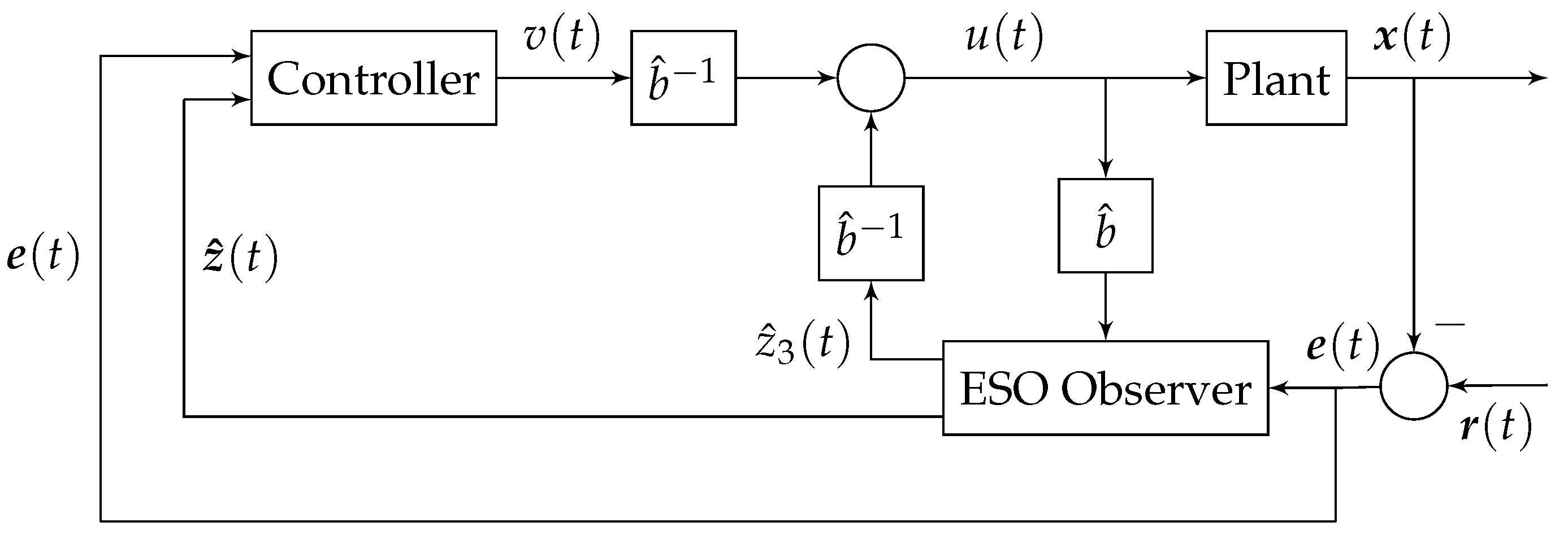
The graphical diagram of the considered system with all appearances of $\widehat{b}$ explicitly shown is given in Figure 1.

Estimation error $\tilde{\mathit{z}}\left(t\right)=\mathit{z}\left(t\right)-\widehat{\mathit{z}}\left(t\right)$ dynamics can now be presented. Dynamics of ${\tilde{z}}_1$ and ${\tilde{z}}_2$ can be calculated straightforward from (3) and (4) as

$$\begin{array}{cc}\hfill {\dot{\tilde{z}}}_1& ={\tilde{z}}_2-k_1{\tilde{z}}_1,\hfill \\ \hfill {\dot{\tilde{z}}}_2& ={\tilde{z}}_3-k_2{\tilde{z}}_1,\hfill \end{array}$$

(7)

while dynamics of ${\tilde{z}}_3$ involves also (5) and is obtained as

$$\begin{array}{cc}\hfill {\dot{\tilde{z}}}_3& =\left(b-\widehat{b}\right)\dot{u}+\frac{d}{dt}\left(\delta -{\ddot{x}}_r\right)-{\dot{\widehat{z}}}_3\hfill \\ \hfill & =\left(b{\widehat{b}}^{-1}-1\right)\left(\dot{v}-{\dot{\widehat{z}}}_3\right)+\frac{d}{dt}\left(\delta -{\ddot{x}}_r\right)-{\dot{\widehat{z}}}_3\hfill \\ \hfill & =\left(b{\widehat{b}}^{-1}-1\right)\dot{v}+\frac{d}{dt}\left(\delta -{\ddot{x}}_r\right)-b{\widehat{b}}^{-1}{k}_3{\tilde{z}}_1.\hfill \end{array}$$

(8)

Please note that ${\dot{\widehat{z}}}_3$ governs ${\dot{\tilde{z}}}_3$ in two-fold manner—once directly through the definition of $\tilde{\mathit{z}}\left(t\right)$ itself and secondly indirectly through the time derivative of control law u. This phenomenon is clearly caused by a possible imperfect choice of $\widehat{b}$ and is cancelled if $\widehat{b}=b$. By substituting (8) to (5) and then into (2) the tracking error $\mathit{e}\left(t\right)$ dynamics can be rewritten as

$$\begin{array}{cc}\hfill {\dot{e}}_1& =e_2,\hfill \\ \hfill {\dot{e}}_2& =v+{\tilde{z}}_3\hfill \end{array}$$

(9)

without any change in their physical interpretation. System (9) can be viewed as a perturbed version of system (6) due to the presence of estimation error ${\tilde{z}}_3$. Equations (7)–(9) can then be expressed in the following compact form

$$\dot{\mathit{\xi }}\left(t\right)=\mathit{H}\mathit{\xi }\left(t\right)+\mathbf{\Gamma }\left(t\right),$$

(10)

where $\mathit{\xi }\left(t\right)={\left[\begin{array}{cc}\tilde{\mathit{z}}{\left(t\right)}^T& \mathit{e}{\left(t\right)}^T\end{array}\right]}^T,$

$$\mathbf{\Gamma }\left(t\right)={\left[\begin{array}{ccccc}0& 0& 1& 0& 0\end{array}\right]}^T\frac{d}{dt}\left(\delta -{\ddot{x}}_r\right),\mathit{H}=\left[\begin{array}{cc}{\mathit{H}}_{\mathrm{obs}}& {\mathit{H}}_1\\ {\mathit{H}}_2& {\mathit{H}}_{\mathrm{reg}}\end{array}\right],$$

(11)

while ${\mathit{H}}_{\mathrm{obs}}\in {\mathbb{R}}^{3\times 3},{\mathit{H}}_{\mathrm{reg}}\in {\mathbb{R}}^{2\times 2}$ and ${\mathit{H}}_1,{\mathit{H}}_2$ are the matrices derived directly from (7)–(9).

Assumption A2.

Let the function δ be continuously differentiable and satisfy $sup∥\frac{d}{dt}\left(\delta \right)∥\le s_{\delta }$ where $s_{\delta }$ is some positive constant.

It is clear that if $\mathit{H}$ is Hurwitz then under the Assumption A1 and A2 the errors in the closed-loop system satisfy the following

$$\underset{t\to \infty }{lim}∥\mathit{\xi }\left(t\right)∥\le \frac{∥\mathit{P}∥}{{\lambda }_{min}\mathit{Q}}sup∥\mathbf{\Gamma }\left(t\right)∥,$$

(12)

where $\mathit{P},\mathit{Q}$ are positive definite symmetrical matrices satisfying the Lyapunov equation ${\mathit{H}}^T\mathit{P}+\mathit{P}\mathit{H}=-\mathit{Q}$. A precise structure of $\mathit{H}$ depends on the chosen structure of the stabilizing control law v. Different choices of this factor will be considered in the following section.

3. Error Dynamics

To apply the control law (5) one needs to use the stabilizing feedback v which can be chosen in multiple ways, with the most common being a simple PD controller. However, its exact form depends on whether the state of the system is measurable or not. Based on this criterion, the following three variants of PD feedback can be distinguished:

• position and velocity errors are estimated

  $$v_{\mathrm{p}}:=-k_{\mathrm{p}}{\widehat{z}}_1-k_{\mathrm{d}}{\widehat{z}}_2,$$

  (13)
• position error is measured while velocity error is estimated

  $$v_{\mathrm{v}}:=-k_{\mathrm{p}}\left(x_1-x_r\right)-k_{\mathrm{d}}{\widehat{z}}_2,$$

  (14)
• position and velocity errors are measured

  $$v_{\mathrm{d}}:=-k_{\mathrm{p}}\left(x_1-x_r\right)-k_{\mathrm{d}}\left(x_2-{\dot{x}}_r\right),$$

  (15)

where $k_{\mathrm{p}},k_{\mathrm{d}}\in \mathbb{R}$ are positive constant input gains.

The considered control structure based on (5) along with feedbacks (13)–(15) diverges from the once commonly accepted in the ADRC methodology, by the lack of reference second derivative ${\ddot{x}}_r$ in the feed-forward path. This property is often given as a major advantage of EADRC approach and will heavily influence results presented in this paper that will be shown in the following paragraphs.

With the stabilizing control law defined, one can consider stability conditions of the closed-loop system. To this end, let us substitute (13)–(15) into (10) to obtain the precise form of system error dynamics matrix ${\mathit{H}}_{\kappa }$, where $\kappa \in \left\{\mathrm{p},\mathrm{v},\mathrm{d}\right\}$ corresponds to the particular feedback $v_{\kappa }$, which can be stated as follows

$${\mathit{H}}_{\mathrm{p}}=\left[\begin{array}{cccc}-k_1& 1& 0\hfill & \\ & & & \\ -k_2& 0& 1\hfill & {\mathit{H}}_1\\ & & & \\ -\beta k_3-\overline{\beta }\left(k_{\mathrm{d}}{k}_{\mathrm{p}}+k_{\mathrm{p}}{k}_1+k_{\mathrm{d}}{k}_2\right)& \overline{\beta }\left(k_{\mathrm{p}}-k_{\mathrm{d}}^2\right)& 0\hfill & \\ 0& 0& 0\hfill \\ & & & {\mathit{H}}_{\mathrm{reg}}\\ k_{\mathrm{p}}& k_{\mathrm{d}}& 1\hfill \end{array}\right],$$

(16)

$${\mathit{H}}_{\mathrm{v}}=\left[\begin{array}{cccc}\hfill -k_1& 1& 0\hfill & \\ & & & \\ \hfill -k_2& 0& 1\hfill & {\mathit{H}}_1\\ & & & \\ \hfill -\beta k_3-\overline{\beta }{k}_{\mathrm{d}}{k}_2& -\overline{\beta }{k}_{\mathrm{d}}^2& 0\hfill & \\ \hfill 0& 0& 0\hfill & \\ & & & {\mathit{H}}_{\mathrm{reg}}\\ \hfill 0& k_{\mathrm{d}}& 1\hfill \end{array}\right],$$

(17)

and

$${\mathit{H}}_{\mathrm{d}}=\left[\begin{array}{cccc}\hfill -k_1& 1& 0\hfill & \\ & & & \\ \hfill -k_2& 0& 1\hfill & {\mathit{H}}_1\\ & & & \\ \hfill -\beta k_3& 0& -\overline{\beta }{k}_{\mathrm{d}}\hfill & \\ \hfill 0& 0& 0\hfill & \\ & & & {\mathit{H}}_{\mathrm{reg}}\\ \hfill 0& 0& 1\hfill \end{array}\right],$$

(18)

where

$${\mathit{H}}_1=\left[\begin{array}{cc}0& 0\\ 0& 0\\ \overline{\beta }{k}_{\mathrm{p}}{k}_{\mathrm{d}}& \overline{\beta }\left(k_{\mathrm{d}}^2-k_{\mathrm{p}}\right)\end{array}\right],{\mathit{H}}_{\mathrm{reg}}=\left[\begin{array}{cc}0& 1\\ -k_{\mathrm{p}}& -k_{\mathrm{d}}\end{array}\right],$$

(19)

$\beta =b{\widehat{b}}^{-1}\in \mathbb{R}$ is a positive constant scaling factor of the nominal b of the plant. Also $\overline{\beta }=\beta -1$ is defined to clear up a notation.

No matter the chosen $v=v_{\kappa }$, vector $\mathbf{\Gamma }\left(t\right)$ remains as is given in (11) what follows from the EADRC approach of defining the extended state vector based on the error domain. In comparison, if the ordinary ADRC technique is used, another form of $\mathbf{\Gamma }\left(t\right)$ emerges in all three cases as

$${\mathbf{\Gamma }}_{\mathrm{ADRC}}\left(t\right)={\left[\begin{array}{ccccc}0& 0& 1& 0& 0\end{array}\right]}^T\left(\frac{d}{dt}\left(\delta \right)+\overline{\beta }\left({\ddot{x}}_r-k_{\mathrm{d}}{\stackrel{⃛}{x}}_r\right)\right).$$

(20)

It is clear that for a vector defined in such a way a choice of parameter value $\beta >1$ leads to an increase of ${\mathbf{\Gamma }}_{\mathrm{ADRC}}\left(t\right)$ norm what, recalling (12), can deteriorate the tracking quality depending on the relative magnitude of reference derivatives and disturbance $\delta \left(t\right)$. For this reason the tuning method proposed in this paper is valid only for the EADRC approach and properties presented in this paper arise as another advantage of the EADRC over ordinary ADRC method.

4. The Stability Analysis of EADRC for the Selected Feedbacks

Stability conditions of $\mathit{H}$ for all variants of v defined by (16)–(18) are now to be investigated. Assume that observer and feedback gains are chosen as

$$\begin{array}{c}{k}_1:={\overline{k}}_1{\omega }_{\mathrm{o}},k_2:={\overline{k}}_2{\omega }_{\mathrm{o}}^2,k_3:={\omega }_{\mathrm{o}}^3,\\ k_{\mathrm{p}}:={\omega }_{\mathrm{c}}^2,k_{\mathrm{d}}:={\overline{k}}_d{\omega }_{\mathrm{c}},\end{array}$$

(21)

where ${\overline{k}}_1$, ${\overline{k}}_2$ are real coefficients of the third-degree polynomial $\varphi \left(\lambda \right)={\lambda }^3+{\overline{k}}_1{\lambda }^2+{\overline{k}}_2\lambda +1$, $\lambda \in \mathbb{C}$, with roots located in the left half-plane of the complex plane, ${\overline{k}}_d>0$ is a nominal derivative feedback gain, while ${\omega }_{\mathrm{o}},{\omega }_{\mathrm{c}}\in \mathbb{R}$ are positive constants used to tune an observer bandwidth and a controller bandwidth, respectively. Although this tuning scheme is designed for the specific case of perfect knowledge of b, it is still justified when $\widehat{b}$ is different from the real value of b. This is due to characteristics of the ADRC approach which makes it possible to shape closed-loop system dynamics according to the assumed reference model [23].

First, the stability of $\mathit{H}$ in the generic case of $\beta \ne 1$ using analytical methods is taken into account. Inspired by results provided by [26] one can consider the following.

Theorem 1.

Let $\mathit{H}$ be defined by (16)–(18), respectively. For the gain parametrization given by (21) and $\beta \in \mathbb{R}$ selected such that

$$\mathit{A}=\left[\begin{array}{ccc}-{\overline{k}}_1& 1& 0\\ -{\overline{k}}_2& 0& 1\\ -\beta & 0& 0\end{array}\right]$$

(22)

is a Hurwitz matrix, there exists a positive constant Ω such that for any ${\omega }_{\mathrm{o}}>\Omega$ the following system

$$\dot{\mathit{\xi }}=\mathit{H}\mathit{\xi },$$

(23)

where $\mathit{\xi }\in {\mathbb{R}}^5$, is asymptotically stable.

Proof. 

To facilitate computations one can consider the following scaling of the state vector in (23)

$${\mathit{\xi }}^{*}=\left[\begin{array}{cc}\mathit{T}& \mathit{0}\\ \mathit{0}& {\mathit{I}}_2\end{array}\right]\mathit{\xi },$$

(24)

where $\mathit{T}=\mathrm{diag}\{1,{\omega }_{\mathrm{o}}^{-1},{\omega }_{\mathrm{o}}^{-2}\}$ and ${\mathit{I}}_m$ denotes the identity matrix of the size of $m\times m$. Recalling the block structure of matrix $\mathit{H}$ specified by (11), one can rewrite dynamics (23) in the new coordinates as

$${\dot{\mathit{\xi }}}^{*}=\left[\begin{array}{cc}{{\mathit{H}}_{\mathrm{obs}}}^{*}& {\mathit{H}}_1^{*}\\ {\mathit{H}}_2^{*}& {\mathit{H}}_{\mathrm{reg}}\end{array}\right]{\mathit{\xi }}^{*},$$

(25)

where the component matrices satisfy

$${{\mathit{H}}_{\mathrm{obs}}}^{*}=\mathit{T}{\mathit{H}}_{\mathrm{obs}}{\mathit{T}}^{-1},{\mathit{H}}_1^{*}=\mathit{T}{\mathit{H}}_1,{\mathit{H}}_2^{*}={\mathit{H}}_2{\mathit{T}}^{-1}.$$

(26)

Considering the particular forms of $\mathit{H}$ defined by (16)–(18), respectively, using (22) and making detailed computations one can show that matrix ${{\mathit{H}}_{\mathrm{obs}}}^{*}$ can be represented as follows

$${{\mathit{H}}_{\mathrm{obs}}}^{*}={\omega }_{\mathrm{o}}\mathit{A}+\overline{\beta }\overline{\mathit{A}},$$

(27)

while

$$\overline{\mathit{A}}=\left[\begin{array}{ccc}0& 0& 0\\ 0& 0& 0\\ a_1\left({\omega }_{\mathrm{o}}\right)& {\omega }_{\mathrm{o}}^{-1}{a}_2& a_3\end{array}\right]$$

(28)

with $a_2$, $a_3$ being constants and $a_1\left({\omega }_{\mathrm{o}}\right)$ denoting a real-valued non-increasing function of ${\omega }_{\mathrm{o}}$. Similarly, matrices ${\mathit{H}}_1^{*}$ and ${\mathit{H}}_2^{*}$ satisfy

$${\mathit{H}}_1^{*}={\omega }_{\mathrm{o}}^{-2}\overline{\beta }{\overline{\mathit{H}}}_1,{\mathit{H}}_2^{*}={\omega }_{\mathrm{o}}^2{\overline{\mathit{H}}}_2,$$

(29)

with

$${\overline{\mathit{H}}}_1=\left[\begin{array}{cc}0& 0\\ 0& 0\\ k_d{k}_p& -k_p+k_d^2\end{array}\right],{\overline{\mathit{H}}}_2=\left[\begin{array}{ccc}0& 0& 0\\ {\omega }_{\mathrm{o}}^{-2}{a}_4& {\omega }_{\mathrm{o}}^{-1}{a}_5& 1\end{array}\right],$$

(30)

where $a_4$ and $a_5$ are constants.

Consider now characteristic polynomial of the state matrix of system (25). Computing this polynomial and taking advantage of properties of the block matrix $\mathit{H}$ one obtains

$$\phi \left(\lambda \right)=det\left({\mathit{I}}_5\lambda -\mathit{H}\right)=det\left({\mathit{I}}_2\lambda -{\mathit{H}}_{\mathrm{reg}}\right)det\left({\mathit{I}}_3\lambda -{{\mathit{H}}_{\mathrm{obs}}}^{*}-{\mathit{H}}_1^{*}{\left({\mathit{I}}_2\lambda -{\mathit{H}}_{\mathrm{reg}}\right)}^{-1}{\mathit{H}}_2^{*}\right).$$

(31)

Using (25) and (29), and making straightforward manipulations one has

$$\phi \left(\lambda \right)={\phi }_{\mathrm{reg}}\left(\lambda \right)det\left({\mathit{I}}_3\lambda -{\omega }_{\mathrm{o}}\left(\mathit{A}-{\omega }_{\mathrm{o}}^{-1}\overline{\beta }\left(\overline{\mathit{A}}+\overline{\overline{\mathit{A}}}\right)\right)\right),$$

(32)

where ${\phi }_{\mathrm{reg}}\left(\lambda \right)=det\left({\mathit{I}}_2\lambda -{\mathit{H}}_{\mathrm{reg}}\right)$ stands for the characteristic polynomial of ${\mathit{H}}_{\mathrm{reg}}$ and

$$\overline{\overline{\mathit{A}}}={\overline{\mathit{H}}}_1{\left({\mathit{I}}_2\lambda +{\mathit{H}}_{\mathrm{reg}}\right)}^{-1}{\overline{\mathit{H}}}_2=\frac{\left(k_d^2-k_p\right)\lambda +k_p{k}_d}{{\phi }_{\mathrm{reg}}\left(\lambda \right)}\left[\begin{array}{ccc}0& 0& 0\\ 0& 0& 0\\ {\omega }_{\mathrm{o}}^{-2}{a}_4& {\omega }_{\mathrm{o}}^{-1}{a}_5& 1\end{array}\right].$$

(33)

It can be found that terms in the second bracket of Equation (32) satisfy the following limit relationship

$$\underset{{\omega }_{\mathrm{o}}\to \infty }{lim}\left(\mathit{A}-{\omega }_{\mathrm{o}}^{-1}\overline{\beta }\left(\overline{\mathit{A}}+\overline{\overline{\mathit{A}}}\right)\right)=\mathit{A}.$$

(34)

Recalling the structure of $\overline{\mathit{A}}$ and $\overline{\overline{\mathit{A}}}$ one can also state that since matrix $\mathit{A}$ is Hurwitz there exists a lower bound $\Omega >0$ a such that for ${\omega }_{\mathrm{o}}>\Omega$ roots of the characteristic polynomial (32) stay in the left half-plane of the complex plane. Hence, one can confirm that for ${\omega }_{\mathrm{o}}>\Omega$ the system (23) is asymptotically stable. □

Remark 1.

The presented theorem can be alternatively understood as an analytical method to approximately find the range of β when the closed-loop system (23) remains stable under the condition that the observer bandwidth is selected high enough. In such a case, the system stability can be evaluated based on characteristics of matrix $\mathit{A}$ which contains the unscaled observer gains, cf. (21). In addition, Theorem 1 covers the particular (nominal) case with $\beta =1$ ($\overline{\beta }=0$) where the stability of the closed-loop systems is satisfied for any positive values of ${\omega }_{\mathrm{o}}$ and ${\omega }_{\mathrm{c}}$.

Considering that Theorem 1 provides the stability result formulated for a high value of ${\omega }_{\mathrm{o}}$, the characteristics of the closed-loop system should be determined also for smaller values of ${\omega }_{\mathrm{c}}$ and ${\omega }_{\mathrm{o}}$. Here, such an analysis is conducted for the gains (21) chosen according to [15] as

$${\overline{k}}_1=3,{\overline{k}}_2=3\mathrm{and}{\overline{k}}_d=2.$$

(35)

To this end, matrix $\mathit{H}$ is analyzed numerically using the Routh-Hurwitz criterion. Results of these computations are shown in Figure 2 with stable regions shown as solid volumes which consist of points above and inside the threshold surface. Analytical form of Routh tables used to calculate these stable regions and additional discussion are presented in Appendix A.

The obtained results have now to be compared with those deduced from Theorem 1. Recalling this theorem for the assumed tuning methodology (21) with (35) one can rewrite matrix (22) as

$$\mathit{A}=\left[\begin{array}{ccc}-3& 1& 0\\ -3& 0& 1\\ -\beta & 0& 0\end{array}\right].$$

(36)

Consequently, it can be found that $\mathit{A}$ is a Hurwitz matrix for $\beta \in \left(0,9\right)$. Hence, it is possible to stabilize the closed-loop system by selecting sufficiently high bandwidth of the observer (${\omega }_{\mathrm{o}}>\Omega$). This result is confirmed by the obtained stable regions for high values of ${\omega }_{\mathrm{o}}$, see Figure 2 . In addition, it is also shown how a choice of bandwidths affects a feasible range of input-gain values. Most importantly, the performed analysis indicates that by employing different stabilizing controllers, especially based on the feedback $v_{\mathrm{d}}$, it is possible to vastly increase the suitable range of $\beta$ parameter. It can be concluded that the character of $\overline{\mathit{A}}$ and $\overline{\overline{\mathit{A}}}$ undergoes a fundamental change with a change of control law v. For $v_{\mathrm{p}}$ and (to a lesser degree) $v_{\mathrm{v}}$ these terms deteriorate the stability of the closed-loop system and with the increase of ${\omega }_{\mathrm{o}}$ the stable region reaches its maximum defined by $\mathit{A}$ matrix. Yet, for $v_{\mathrm{d}}$ these terms seem to improve the overall stability and a mitigation of their influence by an increase of ${\omega }_{\mathrm{o}}$ leads to a reduction of the stable region. As a result, one can judge that main restrictions on the selection of $\beta$ comes from the estimation of velocity error $e_2$ provided by the observer (4) which strongly influences the character of these disturbing matrices.

5. Evaluation of Improving Tracking Accuracy Using Input-Gain Underestimation

Having presented that the parameter $\beta$ can be safely increased in a vast range without decreasing the system stability, practical results of such an increase must be investigated. To this end, multiple simulations were performed. The plant was modelled according to (1) and various scenarios were considered:

• Scenario A—various disturbances and ${\omega }_{\mathrm{o}}=100$, ${\omega }_{\mathrm{c}}=1$

Case A1.

No disturbance, $\delta =0$,

Case A2.

Friction force of the small magnitude, $\delta =-5\left(x_2+sgn{x}_2\right)$,

Case A3.

Friction force of the significant magnitude, $\delta =-15\left(x_2+sgn{x}_2\right)$,

Case A4.

State independent harmonic disturbance, $\delta =10sin\left(32t\right)$.

• Scenario B—various controller bandwidth and ${\omega }_{\mathrm{o}}=100$, $\delta =0$

Case B1.

${\omega }_{\mathrm{c}}=1$,

Case B2.

${\omega }_{\mathrm{c}}=5$,

Case B3.

${\omega }_{\mathrm{c}}=10$,

Case B4.

${\omega }_{\mathrm{c}}=20$.

• Scenario C—various observer bandwidth and ${\omega }_{\mathrm{c}}=1$, $\delta =0$

Case C1.

${\omega }_{\mathrm{o}}=10$,

Case C2.

${\omega }_{\mathrm{o}}=50$,

Case C3.

${\omega }_{\mathrm{o}}=100$,

Case C4.

${\omega }_{\mathrm{o}}=200$.

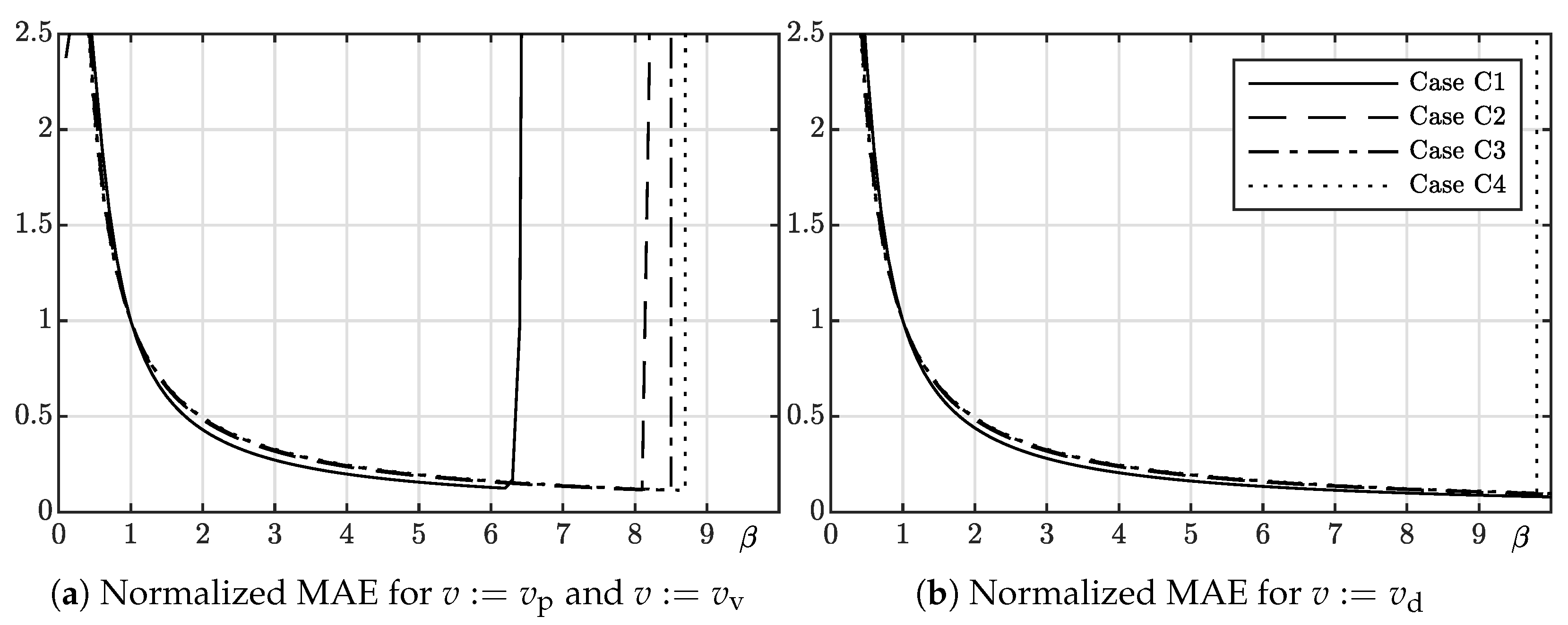
Reference trajectory was designed as a sine wave satisfying $x_r=sin\left(2t\right)$. Series of simulations were performed with such settings for different values of $\beta$ and a MAE criterion of mean absolute error in the steady state was calculated for each scenario as $\mathrm{MAE}=\frac{1}{10}{\int }_{30}^{40}{e}_1\left(t\right)$. Results of the simulations for all variants of v are given in Figure 3, Figure 4 and Figure 5. On each plot, the normalized value of MAE criterion equal to $\frac{\mathrm{MAE}\left(\beta \right)}{\mathrm{MAE}\left(1\right)}$ is presented to visualize influence of the $\beta$-scaling regardless of other parameters chosen for a specific scenario. Plots obtained for variants $v_{\mathrm{p}}$ and $v_{\mathrm{v}}$ proved to be visually identical and were thus merged into one in Figure 3, Figure 4 and Figure 5.

Most importantly, one can see that all plots indicate a significant increase of the tracking quality obtained by the increase of the chosen value of $\beta$ parameter. In contrast to a common assumption used in the ADRC approach, using an underestimated value of $\widehat{b}$ makes it possible to change the tracking performance. Specifically, regardless the selected scenario, one can state that the tracking quality offered by the controller designed in the error domain increases with the input-gain underestimation. The character of this improvement seems to be independent on the chosen disturbance or controller and observer bandwidths. These properties do not hold for the classic ADRC controller, as was explained earlier, and they are the unique characteristic of the EADRC approach.

Remark 2.

The observed improvement of the tracking precision for the EADR structure does not come from an indirect scaling of feedback gains $k_{\mathrm{p}}$ and $k_{\mathrm{d}}$ but from the change of the observer gains. It can be easily deduced from (16)–(18) that β affects the resulting gain of the observer due to the term $\beta k_3$ in the entry (3,1) of matrix ${\mathit{H}}_{\mathrm{obs}}$. However, it is noteworthy that β also scales remaining terms in the third row of ${\mathit{H}}_{\mathrm{obs}}$. Thus, a result of change of parameters β and $k_3$, although can seem to be similar, is not fully equivalent when the stability of the closed-loop system is considered. Moreover, there is a significant practical difference between these two parameters—while the $k_3$ scaling requires a conscious decision of a designer, an input-gain underestimation is often a side effect of an imperfect identification procedure.

Additionally, the upper limit imposed on $\beta$ by the stability conditions of the closed-loop dynamics is clearly visible in Figure 3a,b. The exact value of this threshold changes according to stable regions presented in Figure 2. Interestingly, in Figure 3 one can notice that feasible range of $\beta$ can be extended by energy-dissipating disturbance present in cases A2 and A3 (embodied here as the friction force). Significant extension or lack of such a limit for the $v_{\mathrm{d}}$ is also presented in Figure 3b, Figure 4b and Figure 5b for all scenarios. According to the results in Figure 2c in Figure 5b such a limit is visible for a small value of ${\omega }_{\mathrm{c}}$ (here selected as 1) and a high value of ${\omega }_{\mathrm{o}}$ (here equal to 200). Yet, this limit is significantly greater than for $v:=v_{\mathrm{p}}$ or $v_{\mathrm{v}}$ in Figure 5a.

At last, the practical experiments were performed to confirm the usefulness of the proposed tuning scheme in a real-life application. Tests were carried out using a single axis of a robotic mount of an astronomic telescope with a mirror of diameter of 0.5 m. Some properties of this device, including character of unmodelled disturbances, have been presented in earlier publications [28,29,30]. Based on the previous research, it can be safely assumed that in the slow-motion conditions, friction force is a major disturbance factor in the considered plant. Bandwidths of the observer and controller were chosen as ${\omega }_{\mathrm{o}}=140$ and ${\omega }_{\mathrm{c}}=10$, respectively. The task of trajectory tracking was performed for the trajectories satisfying

$$x_r:=r_v{\left(2\pi r_f\right)}^{-1}sin\left(2\pi r_{f}t\right),$$

(37)

where $r_f=\frac{1}{12}\mathrm{Hz}$ is a sine wave frequency and $r_v$ is a maximum velocity of the reference trajectory chosen as two distinct values depending on the considered case. Experiments were conducted for different structures of stabilizing law v. As was in case of simulations, $v_{\mathrm{p}}$ and $v_{\mathrm{v}}$ provided visually identical results again and were merged into one on the plots. Considered settings were as follows:

Case E1.

estimated state $v:=v_{\mathrm{p}}$ or $v_{\mathrm{v}}$, slow trajectory $r_v:=2\times 7.268\times {10}^{-5}\mathrm{rad}/\mathrm{s}$,

Case E2.

estimated state $v:=v_{\mathrm{p}}$ or $v_{\mathrm{v}}$, fast trajectory $r_v:=2\times 7.268\times {10}^{-2}\mathrm{rad}/\mathrm{s}$.

Case E3.

measured state $v:=v_{\mathrm{d}}$, slow trajectory $r_v:=2\times 7.268\times {10}^{-5}\mathrm{rad}/\mathrm{s}$,

Case E4.

measured state $v:=v_{\mathrm{d}}$, fast trajectory $r_v=2\times 7.268\times {10}^{-2}\mathrm{rad}/\mathrm{s}$.

However, according to the presented analysis, the chosen reference trajectory should not influence the stability of the system, character of the friction force, which constitutes a major part of total disturbance, depends strongly on the velocity of the axis, as the friction passes from a pre-sliding to a sliding regime. This means that the choice of the reference trajectory is here used as an indirect method to change a character of disturbance in the considered system. Results of the experiment in each of the cases is given in Figure 6.

Basically, the obtained experimental results are consistent with the simulation results. It can be found that an increase of the $\widehat{b}$ parameter value improves the tracking quality, as long as this parameter is smaller than some upper-limit value. As was expected, for tests in which $v_{\mathrm{d}}$ feedback was used, this upper limit is significantly greater. No clear loss of stability was observed during the experiments and it is unclear whether rapid decrease of tracking quality at approximately $\widehat{b}\approx 1/120$ for cases 1 and 2 and $\widehat{b}\approx 1/200$ for cases 3 and 4 should be interpreted as an exceeding of this bounding value or is this some other phenomenon, as the overall stability of the plant was maintained even for much bigger values of $\beta$. For a sake of comparison, an additional simulation was performed with ${\omega }_{\mathrm{o}}$ and ${\omega }_{\mathrm{c}}$ chosen as in the experiment and the results are shown in Figure 7. All notations (including simulation cases) in this figure are as in the previous simulations. Value of MAE criterion was not normalized in these figures.

As can be seen, for the chosen gains, loss of the stability in the simulated example happened no earlier than for $\beta \approx 6.8$. If this value indeed corresponds with $\widehat{b}\approx 1/120$ obtained during experiments it would suggest the real value of input gain in the plant not greater than $b\le 1/17.6$. This shows how presented tuning method could be used to estimate some upper bound of a real value of the input gain. Concerning results of the experiments, one must admit that the improvement of the tracking quality obtained with the proposed method was comparable with maximum improvement obtained with traditional method of the bandwidth scaling, i.e., results obtained by the input-gain scaling were comparable with the best results obtained by the increase of ${\omega }_{\mathrm{o}}$ and ${\omega }_{\mathrm{c}}$ only.

6. Conclusions

In the paper new method of the error domain ADRC controller tuning was presented. It was shown that for a significant range of the input-gain underestimation error the closed-loop system remains practically stable, and the tracking errors decrease with an increase of this underestimation. By means of numerical computations it was presented that this feasible range can be made substantially larger by the proper design of the control law. Extensive research by simulations and experiments was carried out to confirm usability of the proposed method and further highlight its properties.

The tuning methodology discussed in this paper has also some limitations. Firstly, it does not clearly provide better tracking quality than other methods based on tuning the observer gains. Secondly, the selection of the high value of the observer bandwidth in real applications is constrained due to the presence of measurement noise and the implementation of the controller and observer in the discrete time domain. However, this remark is more general and can be formulated also with respect to other control structures where high-gain observers are employed.

Despite that, the presented tuning scheme can be seen as an alternative design approach which can be conveniently applied for real control systems. Main practical finding of the paper is that if the input gain is not precisely known, a designer can employ EADRC scheme and consciously set input gain in the controller synthesis as much smaller than the real expected value. Such rule of thumb for controller design allows a designer to partially forsake a demanding process of plant identification and maintain the desired tracking quality.

In future a more complex tuning methodology based on the selection of the input and observer gains can be investigated and compared. In addition, higher order control plants can be taken into account.