On the Sampling of the Fresnel Field Intensity over a Full Angular Sector

Abstract

In this article, the question of how to sample the square amplitude of the radiated field in the framework of phaseless antenna diagnostics is addressed. In particular, the goal of the article is to find a discretization scheme that exploits a non-redundant number of samples and returns a discrete model whose mathematical properties are similar to those of the continuous one. To this end, at first, the lifting technique is used to obtain a linear representation of the square amplitude of the radiated field. Later, a discretization scheme based on the Shannon sampling theorem is exploited to discretize the continuous model. More in detail, the kernel of the related eigenvalue problem is first recast as the Fourier transform of a window function, and after, it is evaluated. Finally, the sampling theory approach is applied to obtain a discrete model whose singular values approximate all the relevant singular values of the continuous linear model. The study refers to a strip source whose square magnitude of the radiated field is observed in the Fresnel zone over a 2D observation domain.

1. Introduction

In the framework of inverse problems in electromagnetics [1,2,3,4,5,6,7], the inverse source problem plays an important role. The latter is a classical problem of the electromagnetic literature [8,9,10,11,12] which consists in recovering the source current from the observation of its radiated field. From the mathematical point of view, the inverse source problem requires to invert a linear integral operator, called a radiation operator, that relates the density current J with the radiated electric field E.

Despite the performances of electronic instrumentation are continuously improved, in some contexts the measure of phase information may be not accurate. Hence, it is worth addressing the problem of reconstructing the source current from amplitude-only data of the radiated field [13,14,15,16,17,18,19,20]. Such a problem falls into the realm of phase retrieval, and it can be formulated as recovering the density current J from the quadratic model:

$${\left|TJ\right|}^2={\left|E\right|}^2$$

(1)

where T stands for the radiation operator.

One of the most popular algorithms to find a solution consists in the minimization of a cost functional obtained by the least-squares problem associated to Equation (1) (see [21,22]). Since the functional to be minimized is quartic, such a method may suffer from the local minima problem.

Different studies have shown that a crucial parameter in the analysis and cure of local minima is played by the dimension of data space M, which represents the number of independent functions that allow expressing the data with a given degree of accuracy [23]. According to such studies [21,24,25], once the number of unknowns N has been fixed, the functional to be minimized becomes more and more similar to a convex one when the dimension of data space M increases. Hence, it will exist a particular value of the dimension of data space such that the functional is free from traps. It is worth noting that the question of quantifying the minimum value of M that ensures the convergence of the least-squares approach is still an open point, since such a value has been found only for some particular mathematical models [24,25,26,27].

In light of the previous discussion, the first aim of this paper is that of evaluating the dimension of data space M and establishing how such quantity is related to the geometrical parameters of the configuration.

Once the dimension of data space will be evaluated, the second goal of this article is that of providing an efficient discretization of the continuous model shown in Equation (1). This study is motivated by the fact that the square amplitude of the radiated field cannot be continuously collected over the observation domain; accordingly, it is of great practical interest to find a discretization scheme that:

• requires a non-redundant number of measurements;
• allows to obtain a discrete model that shares the same mathematical properties of the continuous one.

Such a discretization scheme would bring a series of advantages. On one hand, it would reduce the acquisition time to measure the data, and the memory requirements to store them on the other, it would decrease the computational burden to perform the inversion.

Regarding the sampling of the radiated field E, standard sampling schemes for the case of planar, cylindrical, and spherical scanning are described respectively in [28,29,30]. Despite this, such strategies are not efficient since they require to acquire a number of samples that may be significantly higher than the dimension of data space. Indeed, especially at microwave and millimeter frequencies, the number of required measurements may become extremely high.

In order to reduce the number of measurements, during the years a different sampling scheme (mostly based on a spatially varying spacing) have been developed. Some of them exploit the concept of local bandwidth [31,32,33], others use an adaptive procedure [34,35,36], still others optimize some metrics related to the singular values decomposition of the radiation operator [37,38,39,40,41,42]. In addition to those just mentioned, further sampling techniques used in antenna applications are described in [43,44,45,46,47].

A particularly interesting discretization scheme is the sampling theory approach developed in [45,46]. The latter, under the hypothesis that the operator $T{T}^{†}$ is convolution and band-limited (with $T^{†}$ denoting the adjoint operator of T ), provides not only an efficient sampling of the radiated field (or in other words the grid of points where the data must be collected) but also a strategy to discretize the linear model $TJ=E$.

However, the sampling approach is suitable only for linear problems; hence, it cannot be directly applied in the case of phaseless measurements. With the aim to overcome this issue, the lifting technique [23] can be exploited to recast the quadratic model in (1) as a linear one. Once a linear representation of ${\left|E\right|}^2$ has been obtained, the sampling theory approach can be fruitfully employed to efficiently discretize the continuous model.

Let us stress that the direct applicability of the sampling theory approach is limited to the cases where the operator involved in the correspondent eigenvalue problem is convolution and its kernel is a band-limited function. Hence, when such an operator does not fulfill these properties, the sampling theory approach cannot be directly applied. In such cases, indeed, it can be employed only after a warping transformation has been exploited to recast the kernel of the operator involved in the correspondent eigenvalue problem as a band-limited function of a difference type [48,49,50].

The study developed in this paper will be done with reference to a 2D geometry consisting of a strip electric current observed on an extended observation domain in Fresnel zone.

The paper is organized in the following manner. In Section 2, the geometry of the problem and the correspondent radiation operator are introduced. In Section 3, at first, the lifting operator is defined; after, its analytical properties are studied. In Section 4, the dimension of data space is estimated. In Section 5, a discrete model that approximates the relevant singular values of the lifting operator is provided. A section of conclusions follows.

2. Geometry of the Problem

Let us consider a $2D$ scalar geometry consisting of a source whose density current $\underline{J}\left(x\right)=J\left(x\right){\widehat{i}}_y$ is supported on the set $[-a,a]$ of the x-axis and directed along the y-axis (see Figure 1). Such current radiates an electric field $\underline{E}(r,\theta )=E(r,\theta ){\widehat{i}}_y$ in a homogeneous medium whose wavenumber $\beta$ is given by $\beta =\frac{2\pi }{\lambda }$ with $\lambda$ denoting the wavelength.

The square magnitude of the electric field ${\left|E\right|}^2$ is observed in the Fresnel region on a 2D domain that extends along the polar coordinates $(r,\theta )$ on the set $[r_{min},r_{max}]\times [-{\theta }_{max},{\theta }_{max}]$.

For the considered geometry, the radiated electric field E can by expressed by the equation

$$E(r,u)=TJ\left(x\right)$$

(2)

where $u=sin\left(\theta \right)$, and the radiation operator T is such that

$$T:J\in L_2\left(SD\right)⟶E\in L_4\left(OD\right)$$

(3)

with $L_2\left(SD\right)$ denoting the space of square-integrable functions on $SD=[-a,a]$, and $L_4\left(OD\right)$ indicates the space of functions whose amplitude to the fourth power is integrable on the set $OD=[r_{min},r_{max}]\times [-u_{max},u_{max}]$.

Under the paraxial Fresnel approximation, Equation (2) can be explicitly written as

$$E(r,u)=TJ\left(x\right)=\frac{1}{\sqrt{\beta r}}{e}^{-j\beta r(1+\frac{1}{2}{u}^2)}{\int }_{-a}^{+a}{e}^{-j\frac{\beta }{2r}{x}^2}{e}^{j\beta ux}J\left(x\right)dx.$$

(4)

3. Study of the Lifting Operator

The first aim of this section is that of providing a linear representation of the square magnitude of the radiated field ${\left|E(r,u)\right|}^2$. The introduction of a linear model allows addressing two important tasks. In particular,

• it enables to estimate the dimension of data space by exploiting a singular values approach;
• it allows finding a discrete model that shares the same singular values of the continuous one.

With the aim of obtaining a linear representation of ${\left|E(r,u)\right|}^2$, the lifting technique can be exploited. The latter adopts a redefinition of the unknown space to recast the quadratic model ${\left|TJ\right|}^2={\left|E\right|}^2$ as a linear one. In particular, a linear model is obtained by rewriting Equation (1) in the form below

$${\left|E(r,u)\right|}^2=\left(TJ\right){\left(TJ\right)}^{*}=\frac{1}{\beta r}{\int }_{-a}^{+a}{\int }_{-a}^{+a}{e}^{j\frac{\beta }{2r}({\overline{x}}^2-x^2)}{e}^{-j\beta u(\overline{x}-x)}J\left(x\right)J^{*}{\left(\overline{x}\right)}^{2}dxd\overline{x}$$

(5)

and, by considering as unknown the function

$$F(x,\overline{x})=J\left(x\right)J^{*}\left(\overline{x}\right).$$

(6)

In such a way, the integral operator A which links the unknown function $F(x,\overline{x})$ with the data function ${\left|E(r,u)\right|}^2$ is linear. The latter is known in the literature as the lifting operator and it is defined as

$$A:F\in L_2(SD\times SD)⟶{\left|E\right|}^2\in L_2^{+}\left(OD\right)$$

(7)

where

$$AF=\frac{1}{\beta r}{\int }_{-a}^{+a}{\int }_{-a}^{+a}{e}^{j\frac{\beta }{2r}({\overline{x}}^2-x^2)}{e}^{-j\beta u(\overline{x}-x)}F(x,\overline{x})dxd\overline{x}.$$

(8)

Accordingly, the square magnitude of the radiated electric field can be expressed as

$${\left|E(r,u)\right|}^2=AF(x,\underline{x}).$$

(9)

Once that linear representation of ${\left|E\right|}^2$ has been achieved, our goal is that of addressing the tasks mentioned in points 1 and 2. To this end, it is necessary to introduce the adjoint operator $A^{†}$ and to explicit the auxiliary operator $A{A}^{†}$. Indeed, as well known, the singular values of A are equal to the square root of the eigenvalues of $A{A}^{†}$ [51].

The adjoint operator $A^{†}$ is usually defined as

$$A^{†}(·)={\int }_{r_{min}}^{r_{max}}{\int }_{-u_{max}}^{+u_{max}}\frac{1}{\beta r}{e}^{-j\frac{\beta }{2r}({\overline{x}}^2-x^2)}{e}^{j\beta u(\overline{x}-x)}(·)dudr$$

(10)

where $(·)$ denotes the function of the variables $(r,u)$ on which the adjoint operator acts.

In Appendix A, the integral operator $A{A}^{†}$ is introduced and a closed-form expression of its kernel is provided.

Differently from what is done in Appendix A, here, a weighted adjoint operator $A_w$ is exploited. The latter can be expressed as

$$A_w^{†}(·)={\int }_{r_{min}}^{r_{max}}{\int }_{-u_{max}}^{+u_{max}}\frac{w(x,\overline{x})}{\beta r}{e}^{-j\frac{\beta }{2r}({\overline{x}}^2-x^2)}{e}^{j\beta u(\overline{x}-x)}(·)dudr$$

(11)

where $w(x,\overline{x})$ represents a weight function.

On the one hand, the use of a weighted adjoint will allow simplifying the mathematical discussion and on the other, it will bring a change of the singular values of the lifting operator. Despite this, such changes will affect only the dynamics of the singular values but not the critical index at which they become negligible. Hence, for our purposes, the effect brought by the weight function can be neglected.

Anyway, the main difference with what is done in Appendix A is that, here, the kernel of the operator $A{A}_w^{†}$ will be expressed as a double integral and not as the square amplitude of a one-dimensional integral. This new representation of the kernel of $A{A}_w^{†}$ will suggest to introduce a change of variables or better a warping transformation that allows rewriting it like the Fourier transform of a constant function defined on a two-dimensional finite domain. On the basis of such discussion, it follows that:

• the eigenvalues of $A{A}_w^{†}$ can be computed in closed-form by resorting to the Slepian Pollak theory;
• the kernel of $A{A}_w^{†}$ will be not only convolution but also band-limited, hence, the sampling theory approach will be fruitful to find a discretization of the correspondent eigenvalue problem.

Note that the idea of exploiting a warping transformation with the aim to recast the kernel of an operator like the Fourier transform of a window function has been already exploited in other recent works [48,49,50].

In order to formalize the above discussion from a mathematical point of view, let us explicit the operator $A{A}_w^{†}$. The latter is given by

$$A{A}_w^{†}(·)={\int }_{r_{min}}^{r_{max}}{\int }_{-u_{max}}^{+u_{max}}\overline{H}(r,r_o,u,u_o)(·)dudr$$

(12)

where:

$$\overline{H}(r,r_o,u,u_o)=\frac{1}{{\beta }^{2}r{r}_o}{\int }_{-a}^{+a}{\int }_{-a}^{+a}w(x,\overline{x})e^{j\frac{\beta }{2}\left(\frac{1}{r_o}-\frac{1}{r}\right)({\overline{x}}^2-x^2)}{e}^{-j\beta (u_o-u)(\overline{x}-x)}dxd\overline{x}.$$

(13)

Now, let us divide the integration domain $S=[-a,a]\times [-a,a]$ as made below

$$S=S_1\cup S_2$$

where $S_1=\{(x,\overline{x})\in S:x\ne \overline{x}\}$, $S_2=\{(x,\overline{x})\in S:x=\overline{x}\}$.

Since $S_2$ is a null set with respect to the Lebesgue measure, the kernel $\overline{H}(r,r_o,u,u_o)$ can be computed by performing the integration only on $S_1$. This means that

$$\begin{array}{c}\hfill \overline{H}(r,r_o,u,u_o)=\frac{1}{{\beta }^{2}r{r}_o}{\int \int }_{S_1}w(x,\overline{x})e^{j\frac{\beta }{2}\left(\frac{1}{r_o}-\frac{1}{r}\right)({\overline{x}}^2-x^2)}{e}^{-j\beta (u_o-u)(\overline{x}-x)}dxd\overline{x}.\end{array}$$

(14)

With the aim to express the kernel through a Fourier Transform relation, it is possible to introduce the following transformation

$$\left\{\begin{array}{c}{X}_1=\overline{x}-x\\ X_2={\displaystyle \frac{{\overline{x}}^2-x^2}{r_{max}}}.\end{array}\right.$$

(15)

The latter is injective and continuously differentiable on $S_1$ and, it allows rewriting the kernel of $A{A}_w^{†}$ in the following form

$$\overline{H}(r,r_o,u,u_o)={\displaystyle \frac{1}{{\beta }^{2}r{r}_o}}{\int \int }_{{\Sigma }_1}w(X_1,X_2)e^{j\frac{\beta }{2}\left(\frac{r_{max}}{r_o}-\frac{r_{max}}{r}\right)X_2}{e}^{-j\beta (u_o-u)X_1}\left|\frac{\partial (x,\overline{x})}{\partial (X_1,X_2)}\right|d{X}_{1}d{X}_2$$

(16)

where

• ${\Sigma }_1$ denotes the new domain in which the original integration domain $S_1$ is mapped by trasformation (15),
• $\left|\frac{\partial (x,\overline{x})}{\partial (X_1,X_2)}\right|=-{\displaystyle \frac{r_{max}}{2X_1}}$ is the Jacobian determinant of the transformation.

Let us remark that, despite $\left|\frac{\partial (x,\overline{x})}{\partial (X_1,X_2)}\right|$ being singular for $X_1=0$, such point does not belong to the integration domain ${\Sigma }_1$. Hence, the integrand in (16) is free from singularities.

At this point, let us choose the weight function $w(X_1,X_2)$. By fixing

$$w(X_1,X_2)={\left(\left|\frac{\partial (x,\overline{x})}{\partial (X_1,X_2)}\right|\right)}^{-1}=-{\displaystyle \frac{2X_1}{r_{max}}}$$

(17)

it results that

$$\overline{H}(r,r_o,u,u_o)={\displaystyle \frac{1}{{\beta }^{2}r{r}_o}}{\int \int }_{{\Sigma }_1}{e}^{j\frac{\beta }{2}\left(\frac{r_{max}}{r_o}-\frac{r_{max}}{r}\right)X_2}{e}^{-j\beta (u_o-u)X_1}d{X}_{1}d{X}_2.$$

(18)

Equation (18) shows that the kernel of $A{A}_w^{†}$ can be seen as the Fourier transform of a constant function defined on the set ${\Sigma }_1$. The shape of the set ${\Sigma }_1$ is depicted in Figure 2.

As seen from Figure 2, the integration domain ${\Sigma }_1$ is not rectangular. However, since the area of ${\Sigma }_1$ does not differ significantly from the area of the smallest rectangular that encloses ${\Sigma }_1$, $\overline{H}(r,r_o,u,u_o)$ can be evaluated by integrating on the smallest rectangle that includes the set ${\Sigma }_1$. The latter is made up by all the points $(X_1,X_2)$ belonging to the rectangular set $[-2a,2a]\times [-a^2/r_{max},a^2/r_{max}]$.

By performing the integration on such domain, it results that

$$\overline{H}(r,r_o,u,u_o)\approx \frac{8a^3}{{\beta }^2{r}_{max}}{\displaystyle \frac{1}{r{r}_o}}sinc\left(\frac{\beta a^2}{2}\left(\frac{1}{r_o}-{\displaystyle \frac{1}{r}}\right)\right)sinc\left(2\beta a(u_o-u)\right).$$

(19)

Accordingly, the operator $A{A}_w^{†}$ can be expressed as

$$\begin{array}{c}\hfill A{A}_w^{†}(·)\approx {\displaystyle \frac{8a^3}{{\beta }^2{r}_{max}}}{\int }_{r_{min}}^{r_{max}}{\int }_{-u_{max}}^{+u_{max}}\frac{1}{r{r}_o}sinc\left(\frac{\beta a^2}{2}\left(\frac{1}{r_o}-\frac{1}{r}\right)\right)sinc\left(2\beta a(u_o-u)\right)(·)dudr.\end{array}$$

(20)

From (20), it is evident that the operator $A{A}_w^{†}$ becomes more similar to a convolution operator if $s=r_{max}/r$ is set. In fact, by doing this, it follows that

$$\begin{array}{c}\hfill A{A}_w^{†}(·)\approx {\displaystyle \frac{8a^3}{{\beta }^2{r}_{max}^2}}{\int }_{s_{min}}^{s_{max}}{\int }_{-u_{max}}^{+u_{max}}{\displaystyle \frac{s_o}{s}}sinc\left({\displaystyle \frac{\beta a^2}{2r_{max}}}\left(s_o-s\right)\right)sinc\left(2\beta a(u_o-u)\right)(·)duds\end{array}$$

(21)

where $s_{min}=1$, $s_{max}=r_{max}/r_{min}$.

The last equation provides an approximated form of the operator $A{A}_w^{†}$ which will be used in next sections to estimate the dimension of data space, and to find a discrete model that shares the same mathematical properties of the continuous one.

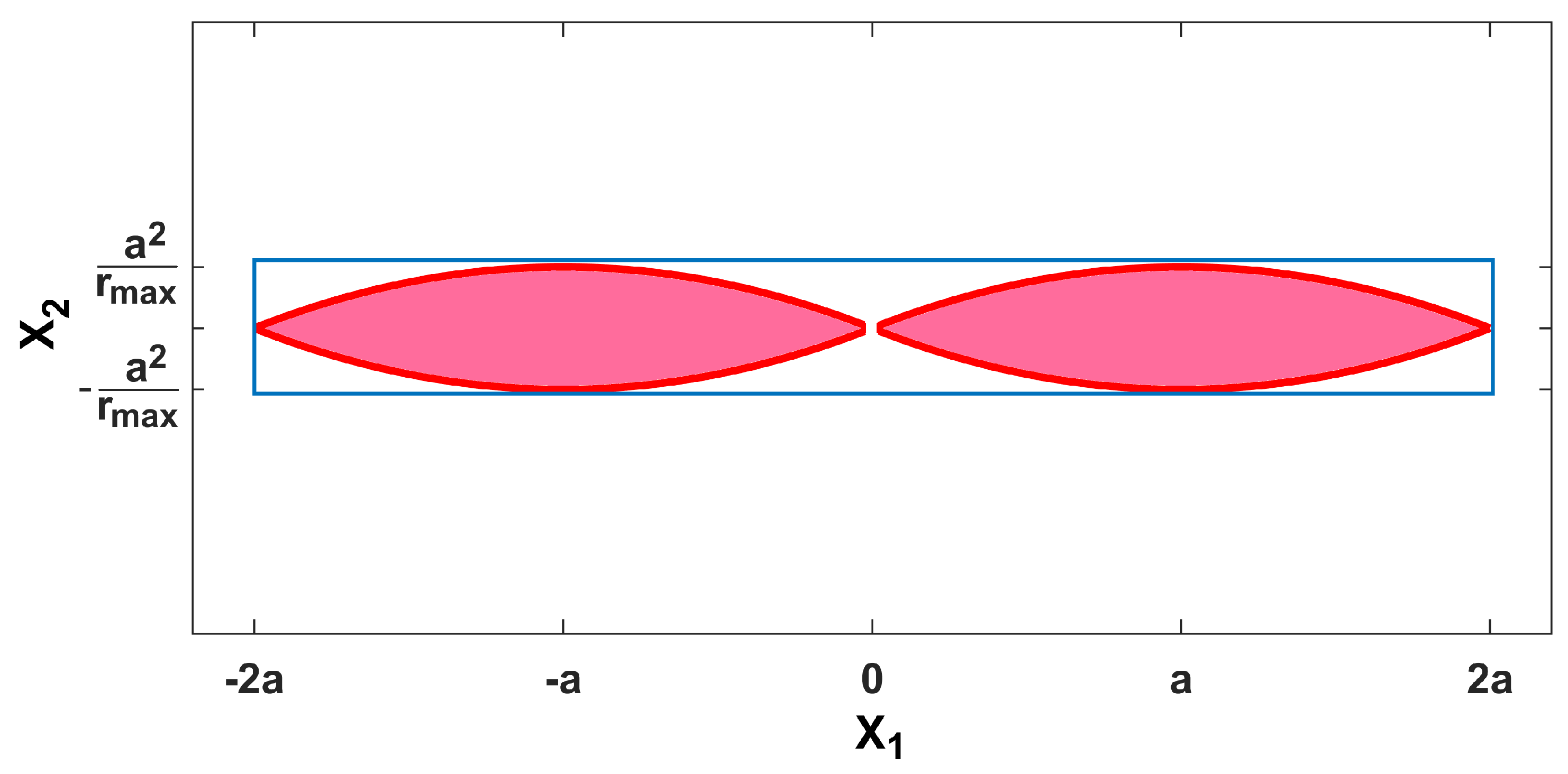
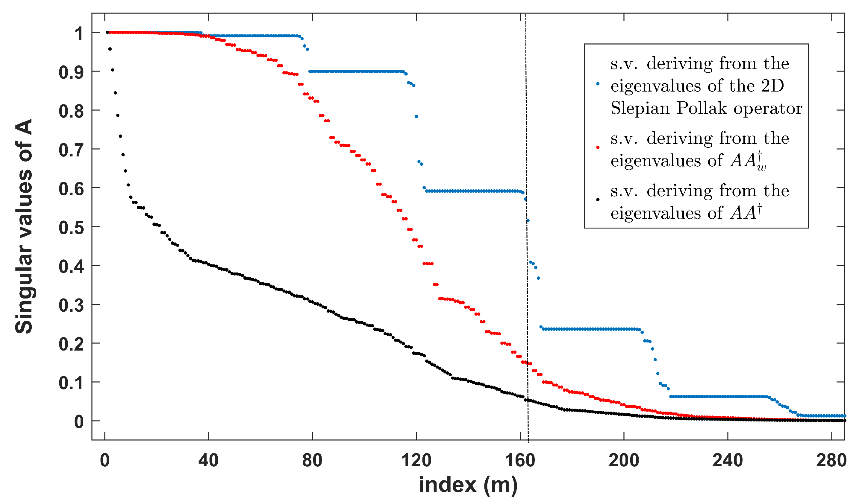
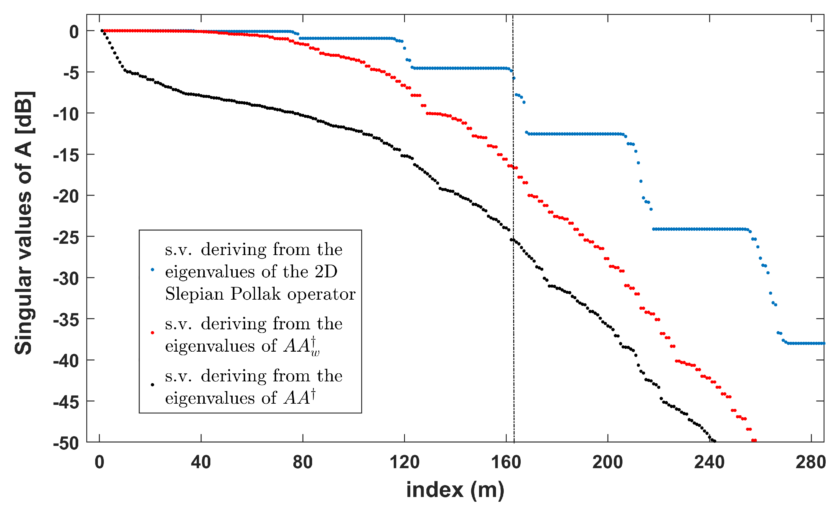
4. Estimation of the Dimension of Data

In this section, an analytical evaluation of the dimension of data space is provided. Different methods can be exploited to achieve this task, here, an SVD-based approach that allows estimating the dimension of data space by counting the number of significant singular values of the lifting operator A is exploited [52].

As is well known, the singular values of A, $\left\{{\sigma }_m\right\}$, are related to the eigenvalues of $A{A}^{†}$, $\left\{{\lambda }_m^{\prime }\right\}$, by the equation

$${\sigma }_m\left(A\right)=\sqrt{{\lambda }_m^{\prime }\left(A{A}^{†}\right)}.$$

(22)

However, only the eigenvalues of $A{A}_w^{†}$ are known in closed-form. For such a reason, at first, it will be solved by the eigenvalue problem

$$A{A}_w^{†}{v}_m={\lambda }_m{v}_m$$

(23)

where ${\lambda }_m$ and $v_m$ are respectively the eigenvalues, and the eigenfunctions of $A{A}_w^{†}$. After, through a numerical analysis, it will be checked that the number of relevant eigenvalues of $A{A}_w^{†}$ is essentially the same as the number of relevant eigenvalues of $A{A}^{†}$.

To evaluate the eigenvalues of $A{A}_w^{†}$, let us explicit Equation (23) as below

$${\displaystyle \frac{8a^3}{{\beta }^2{r}_{max}^2}}{\int }_{s_{min}}^{s_{max}}{\int }_{-u_{max}}^{+u_{max}}{\displaystyle \frac{s_o}{s}}sinc\left({\displaystyle \frac{\beta a^2}{2r_{max}}}\left(s_o-s\right)\right)sinc\left(2\beta a(u_o-u)\right)v_m(s,u)duds={\lambda }_m{v}_m(s_o,u_o).$$

(24)

By fixing

$${\tilde{v}}_m(s,u)={\displaystyle \frac{v_m(s,u)}{s}},$$

(25)

Equation (24) can be recast as

$${\displaystyle \frac{8a^3}{{\beta }^2{r}_{max}^2}}{\int }_{s_{min}}^{s_{max}}{\int }_{-u_{max}}^{u_{max}}sinc\left({\displaystyle \frac{\beta a^2}{2r_{max}}}\left(s_o-s\right)\right)sinc\left(2\beta a(u_o-u)\right){\tilde{v}}_m(s,u)duds={\lambda }_m{\tilde{v}}_m(s_o,u_o).$$

(26)

The eigenvalues of (26) were computed in closed-form in [53], and they are given by

$${\lambda }_m\left(A{A}_w^{†}\right)={\lambda }_{m_1}^{\left(u\right)}{\lambda }_{m_2}^{\left(s\right)}$$

(27)

where ${\lambda }_{m_1}^{\left(u\right)}$ and ${\lambda }_{m_2}^{\left(s\right)}$ denote the eigenvalues of the Slepian–Pollak operators whose kernels are respectively $sinc\left(2\beta a(s_o-s)\right)$ and $sinc\left(\frac{\beta a^2}{2r_{max}}(s_o-s)\right)$. Since the sequences $\{{\lambda }_{m_1}^{\left(u\right)}\}$ and $\{{\lambda }_{m_2}^{\left(s\right)}\}$ are relevant respectively until the indexes

$$M_u={\displaystyle \frac{4}{\pi }}\beta a{u}_{max}+1M_s={\displaystyle \frac{\beta a^2}{2\pi }}\left({\displaystyle \frac{1}{r_{min}}}-{\displaystyle \frac{1}{r_{max}}}\right)+1,$$

(28)

it results that the eigenvalues of the problem (26) and, consequently, the eigenvalues of the operator $A{A}_w^{†}$ are significant until the index

$$\overline{M}=M_u{M}_s.$$

(29)

Let us recall that the kernel of the operator $A{A}_w^{†}$ has been computed by integrating on the smallest rectangular that encloses ${\Sigma }_1$. For such a reason, the scalar $\overline{M}$ is not exactly equal to the number of relevant eigenvalues of $A{A}_w^{†}$ but it represents an upper bound.

In the first part of this section, the eigenvalues behavior of $A{A}_w^{†}$ has been found, however, the actual singular values of A are equal to the square root of the eigenvalues of $A{A}^{†}$. This means that only an approximation of the singular values of A given by the square root of the eigenvalues of $A{A}_w^{†}$ is known.

Now, by means of numerical experiments, it is checked that actual singular values of A and its approximated version computed starting from the eigenvalues of $A{A}_w^{†}$ become negligible at the same index.

As a test case, a configuration in which $a=10\lambda$, $u_{max}=0.5$, $r_{min}=25\lambda$ ($s_{max}=4$), $r_{max}=100\lambda$ and ($s_{min}=1$) is considered. With reference to such a configuration, in Figure 3 and Figure 4 the actual singular values of A and their approximation in the sense clarified above are sketched in natural scale and in dB. In particular, the blue, red, and black diagrams sketch respectively:

• the square root of the eigenvalues of the approximated version of $A{A}_w^{†}$ provided by (21),
• the square root of the eigenvalues of $A{A}_w^{†}$,
• the square root of the eigenvalues of $A{A}^{†}$.

As can be seen from Figure 3 and Figure 4, the square root of the eigenvalues of Operator (21) exhibits a multi-step behavior and it is relevant until index $\overline{M}=M_u{M}_s=164$.

However, our aim is to predict the critical index at which the actual singular values of A become negligible. By observing the behavior of the actual singular values (black diagram in Figure 3 and Figure 4), it is evident that the singular values beyond index $\overline{M}=164$ are surely negligible while those before are almost all significant if the noise level is not so high. This implies that the use of the weighted adjoint changes only the dynamics of the singular values but not the critical index at which they become negligible. For such a reason, it is possible to state that $\overline{M}=M_u{M}_s$ is an upper bound for the dimension of data space that is very close to its actual value.

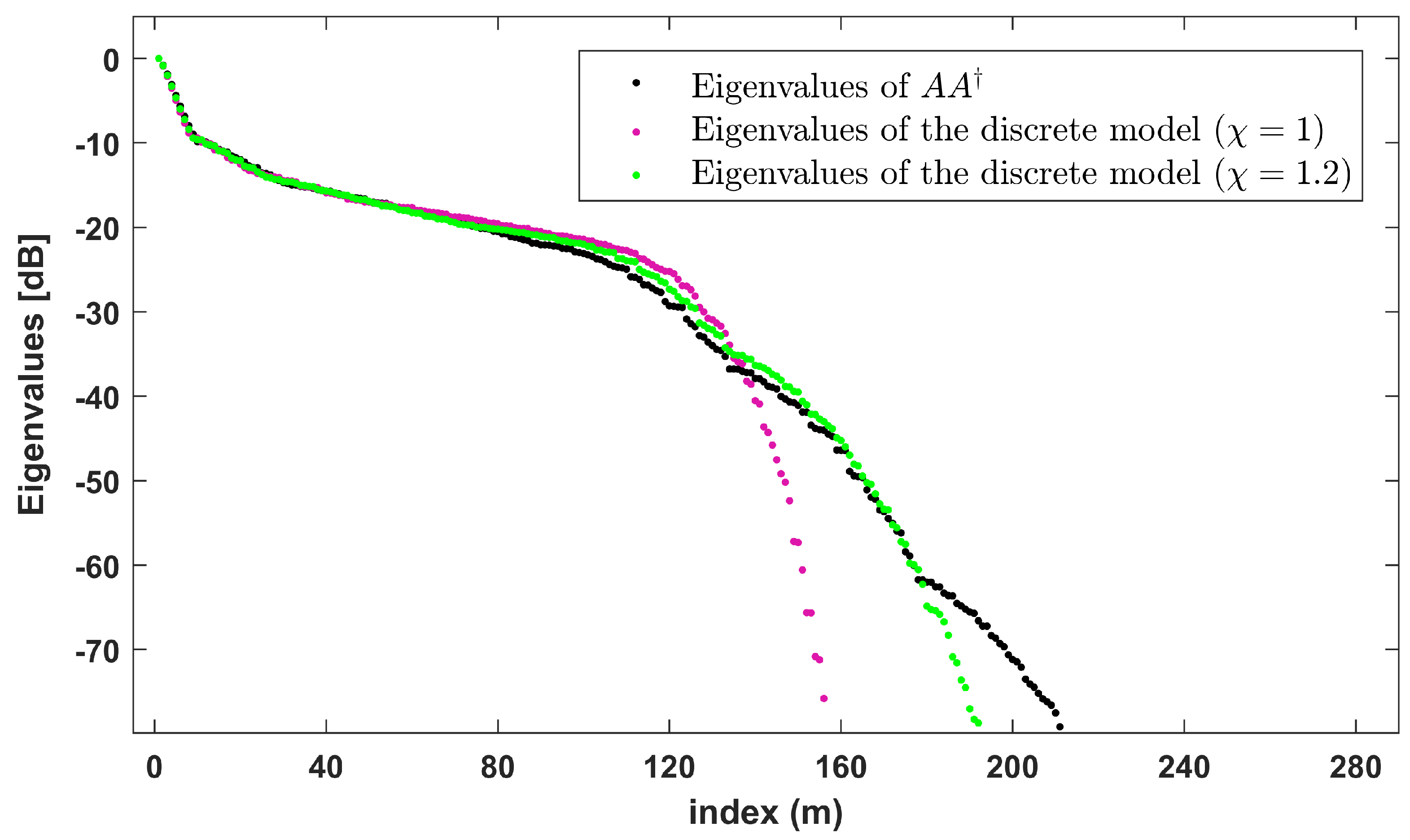
5. Sampling Approach

In this section, the problem of how to discretize the continuous model $AF={\left|E\right|}^2$ in such a way that the discrete model approximates the most important singular values of the continuous model is addressed.

Since the singular values of A are the square root of the eigenvalues of $A{A}^{†}$, this task can be recast as finding a proper discretization of the eigenvalue problem

$$A{A}^{†}{v}_m^{\prime }={\lambda }_m^{\prime }{v}_m^{\prime }$$

(30)

where $v_m^{\prime }$ stands for the eigenfunctions of $A{A}^{†}$.

For the sake of simplicity, instead of discretizing Equation (30), a discretization of the eigenvalue problem $A{A}_w^{†}{v}_n={\lambda }_m{v}_n$ that approximates all the relevant eigenvalues of $A{A}_w^{†}$ will be found. Afterwards, by means of some numerical simulations, it will be checked that the discretization scheme adopted for the operator $A{A}_w^{†}$ works also for $A{A}^{†}$.

As shown in Section 4, by fixing ${\tilde{v}}_m(s,u)=v_m(s,u)/s$, the eigenvalue problem $A{A}_w^{†}{v}_m={\lambda }_m{v}_m$ can be recast as

$${\int }_{s_{min}}^{s_{max}}{\int }_{-u_{max}}^{u_{max}}\tilde{H}(s,s_o,u,u_o){\tilde{v}}_m(s,u)duds={\lambda }_m{\tilde{v}}_m(s_o,u_o)$$

(31)

where

$$\tilde{H}(s,s_o,u,u_o)={\displaystyle \frac{8a^3}{{\beta }^2{r}_{max}^2}}sinc\left({\displaystyle \frac{\beta a^2}{2r_{max}}}\left(s_o-s\right)\right)sinc\left(2\beta a(u_o-u)\right).$$

(32)

The continuous model in (31) involves a convolution operator with a band-limited kernel, accordingly, it can be discretized by exploiting the sampling theory approach developed in [45,46].

A key role in the discretization process is played by the sampling frequency. Since the bandwidth of the kernel function with respect to the variables $u_o$ and $s_o$ is given by $W_u=2\beta a$ and $W_s=\beta a^2/2r_{max}$, the sampling steps $\Delta u$ and $\Delta s$ to be used in the discretization process must satisfy the conditions

$$\Delta u={\displaystyle \frac{\pi }{\chi W_u}}={\displaystyle \frac{\pi }{2\chi \beta a}}\Delta s={\displaystyle \frac{\pi }{\chi W_s}}={\displaystyle \frac{2\pi r_{max}}{\chi \beta a^2}}$$

(33)

where $\chi \ge 1$ is an eventually oversampling factor.

The application of the sampling theory approach provides the following discrete model

$$\underline{\underline{L}}{\underline{\tilde{v}}}_m={\lambda }_m{\underline{\tilde{v}}}_m$$

(34)

where

• $\underline{\underline{L}}$ is a matrix made up by the scalars $L_{pqij}$ given by

  $$L_{pqij}={\int }_{s_{min}}^{s_{max}}{\int }_{-u_{max}}^{u_{max}}\tilde{H}(s,s_{o_p},u,u_{o_q})sinc\left({\displaystyle \frac{\pi }{\Delta s}}(s-s_i)\right)sinc\left({\displaystyle \frac{\pi }{\Delta u}}(u-u_j)\right)duds$$

  (35)
• ${\underline{\tilde{v}}}_m$ is the vector whose elements are the samples of the eigenfunction ${\tilde{v}}_m(u,s)$.

In Appendix B, all the mathematical steps that allow passing from the continuous Model (31) to the discrete Model (34) are shown.

According to [45,46], apart for the truncation error in the sampling expansion, the matrix $\underline{\underline{L}}$ exhibits the same eigenvalues of the continuous model.

Let us point out that the dimension of matrix $\underline{\underline{L}}$ and of the vector ${\underline{\tilde{v}}}_m$ are equal to the number of sampling functions $\tilde{M}$ used in the expansion of the kernel function and of the eigenfunctions. Since, in our case, only the sampling functions corresponding to the samples falling into the set $[-u_{max},u_{max}]\times [s_{min},s_{max}]$ has been considered, it results that

$$\tilde{M}={\tilde{M}}_u{\tilde{M}}_s$$

(36)

where

$${\tilde{M}}_u={\displaystyle \frac{2u_{max}}{\Delta u}}+1={\displaystyle \frac{4}{\pi }}\chi \beta a{u}_{max}+1$$

(37)

$${\tilde{M}}_s={\displaystyle \frac{\chi \beta a^2}{2\pi }}\left({\displaystyle \frac{1}{r_{min}}}-{\displaystyle \frac{1}{r_{max}}}\right)+1.$$

(38)

As can be seen from the Equations (36)–(38), if $\chi =1$ then the number of samples $\tilde{M}$ which fall into the domain $[-u_{max},u_{max}]\times [s_{min},s_{max}]$ is exactly equal to $\overline{M}$, the upper bound to the dimension of data space provided in Section 4.

However, as specified before, our aim is that of finding an efficient discretization of $A{A}^{†}$. For such reason, it is verified if the sampling steps $\Delta u$ and $\Delta s$ used in the discretization of $A{A}_w^{†}$ work also for $A{A}^{†}$.

Figure 5 shows the eigenvalues of $A{A}^{†}$, and those of the correspondent discrete models obtained by using as sampling steps $(\Delta u=\pi /W_u,\Delta s=\pi /W_s)$ and $(\Delta u=\pi /\left(1.2W_u\right),\Delta s=\pi /\left(1.2W_s\right))$. As can be seen from Figure 5, a sampling frequency exactly equal to the Nyquist rate is already sufficient to approximate the most important eigenvalues of $A{A}^{†}$; instead, a sampling frequency higher than the Nyquist rate allows for also approximating the eigenvalues whose value is lower.

It is interesting to highlight that the sampling approach returns also the locations where the phaseless data (the square amplitude of the electric field) must be collected. The latter are given by all the possible couples $(s_o,u_o)$ such that

$$s_o=s_{min}+p\Delta s\mathrm{with}p=1,2,\dots ,{\tilde{M}}_s$$

(39)

$$u_o=-u_{max}+q\Delta u\mathrm{with}q=1,2,\dots ,{\tilde{M}}_u.$$

(40)

Naturally, each couple $(s_o,u_o)$ is mapped in a couple $(r_o,{\theta }_o)$. The latter can be easily computed by remembering that $u_o=sin{\theta }_o$ and $s_o=r_{max}/r_o$. Since the relations linking $u_o$ with ${\theta }_o$, and $s_o$ with $r_o$ are bot nonlinear, the uniform sampling in the variables $(s_o,u_o)$ is mapped into a spatially varying sampling in the variables $(r_o,{\theta }_o)$. Such behavior is confirmed also by Figure 6 which sketches the grid of the optimal sampling points in the case $\chi =1$.

6. Conclusions

In this article, two issues which fall into the realm of phaseless inverse source problem were addressed. The first one was that of estimating analytically the dimension of data space by means of the singular value decomposition of the lifting operator. The second one was that of introducing a strategy to collect the phaseless data. In particular, in regards to the first point, a good upper bound to the dimension of data space is provided and the relation between the dimension of data space, the frequency, and the geometrical parameters of the configuration found. In regards to the second point, a discretization strategy that allows obtaining a discrete model whose singular values approximate very well the most important singular values of the lifting operator was introduced.

The analysis was performed in the case of a 2D scalar geometry consisting of a strip electric current observed on a two dimensional observation domain in Fresnel zone.

References

1. Chen, X. Computational Methods for Electromagnetic Inverse Scattering; John Wiley & Sons: New York, NY, USA, 2018. [Google Scholar]
2. Rehman, O.U.; Rehman, S.U.; Tu, S.; Khan, S.; Waqas, M.; Yang, S. A Quantum Particle Swarm Optimization Method With Fitness Selection Methodology for Electromagnetic Inverse Problems. IEEE Access 2018, 6, 63155–63163. [Google Scholar] [CrossRef]
3. Brown, T.; Vahabzadeh, Y.; Caloz, C.; Mojabi, P. Electromagnetic Inversion With Local Power Conservation for Metasurface Design. IEEE Antennas Wirel. Propag. Lett. 2020, 19, 1291–1295. [Google Scholar] [CrossRef]
4. Dell’Aversano, A.; Leone, G.; Ciaramaglia, F.; Solimene, R. A Strategy for Reconstructing Simple Shapes From Undersampled Backscattered Data. IEEE Geosci. Remote Sens. Lett. 2016, 13, 1757–1761. [Google Scholar] [CrossRef]
5. Ji, X.; Liu, X. Inverse electromagnetic source scattering problems with multifrequency sparse phased and phaseless far field data. SIAM J. Sci. Comput. 2019, 41, B1368–B1388. [Google Scholar] [CrossRef] [Green Version]
6. Brancaccio, A.; Solimene, R. Fault detection in dielectric grid scatterers. Opt. Express 2015, 23, 8200–8215. [Google Scholar] [CrossRef]
7. Akbari Sekehravani, E.; Leone, G.; Pierri, R. NDF of Scattered Fields for Strip Geometries. Electronics 2021, 10, 202. [Google Scholar] [CrossRef]
8. Karamehmedović, M.; Kirkeby, A.; Knudsen, K. Stable source reconstruction from a finite number of measurements in the multi-frequency inverse source problem. Inverse Probl. 2018, 34, 065004. [Google Scholar] [CrossRef] [Green Version]
9. Cuccaro, A.; Solimene, R. Inverse source problem for a host medium having pointlike inhomogeneities. IEEE Trans. Geosci. Remote Sens. 2018, 56, 5148–5159. [Google Scholar] [CrossRef]
10. Lopéz, Y.A.; Andres, F.L.H.; Pino, M.R.; Sarkar, T.K. An improved super-resolution source reconstruction method. IEEE Trans. Instrum. Meas. 2009, 58, 3855–3866. [Google Scholar] [CrossRef]
11. Foged, L.J.; Scialacqua, L.; Saccardi, F.; Quijano, J.A.; Vecchi, G.; Sabbadini, M. Practical application of the equivalent source method as an antenna diagnostics tool. IEEE Antennas Propag. Mag. 2012, 54, 243–249. [Google Scholar] [CrossRef]
12. Leone, G. Source geometry optimization for hemispherical radiation pattern coverage. IEEE Trans. Antennas Propag. 2016, 64, 2033–2038. [Google Scholar] [CrossRef]
13. Brown, T.; Jeffrey, I.; Mojabi, P. Multiplicatively Regularized Source Reconstruction Method for Phaseless Planar Near-Field Antenna Measurements. IEEE Trans. Antennas Propag. 2017, 65, 2020–2031. [Google Scholar] [CrossRef]
14. Wang, X.; Konno, N.K.; Chen, Q. Diagnosis of Array Antennas Based on Phaseless Near-Field Data Using Artificial Neural Network. IEEE Trans. Antennas Propag. 2020. [Google Scholar] [CrossRef]
15. Wang, L.; Zhang, Y.; Han, F.; Zhou, J.; Liu, Q.H. A Phaseless Inverse Source Method (PISM) Based on Near-Field Scanning for Radiation Diagnosis and Prediction of PCBs. IEEE Trans. Microw. Theory Tech. 2020, 68, 4151–4160. [Google Scholar] [CrossRef]
16. Álvarez, Y.; Las-Heras, F.; Pino, M.R. The Sources Reconstruction Method for Amplitude-Only Field Measurements. IEEE Trans. Antennas Propag. 2010, 58, 2776–2781. [Google Scholar] [CrossRef]
17. Battaglia, G.M.; Palmeri, R.; Morabito, A.F.; Nicolaci, P.G.; Isernia, T. A Non Iterative Crosswords Inspired Approach to the Recovery of 2D Discrete Signals from Phaseless Fourier Transform Data. IEEE Open J. Antennas Propag. 2021, 2, 269–280. [Google Scholar] [CrossRef]
18. Kornprobst, J.; Paulus, A.; Knapp, J.; Eibert, T.F. Phase Retrieval for Partially Coherent Observations. IEEE Trans. Signal Process. 2021, 69, 1394–1406. [Google Scholar] [CrossRef]
19. Razavi, S.F.; Rahmat-Samii, Y. A new look at phaseless planar near-field measurements: Limitations, simulations, measurements, and a hybrid solution. IEEE Antennas Propag. Mag. 2007, 49, 170–178. [Google Scholar] [CrossRef]
20. García-Fernández, M.; López, Y.Á.; Arboleya, A.; González-Valdés, B.; Rodríguez-Vaqueiro, Y.; Gómez, M.E.D.C.; Andrés, F.L.H. Antenna diagnostics and characterization using unmanned aerial vehicles. IEEE Access 2017, 5, 23563–23575. [Google Scholar] [CrossRef]
21. Isernia, T.; Leone, G.; Pierri, R. Radiation pattern evaluation from near-field intensities on planes. IEEE Trans. Antennas Propag. 1996, 44, 701. [Google Scholar] [CrossRef]
22. Qian, J.; Yang, C.; Schirotzek, A.; Maia, F.; Marchesini, S. Efficient algorithms for ptychographic phase retrieval. Inverse Probl. Appl. Contemp Math 2014, 615, 261–280. [Google Scholar]
23. Moretta, R.; Pierri, R. Performance of Phase Retrieval via Phaselift and Quadratic Inversion in Circular Scanning Case. IEEE Trans. Antennas Propag. 2019, 67, 7528–7537. [Google Scholar] [CrossRef]
24. Sun, J.; Qu, Q.; Wright, J. A geometric analysis of phase retrieval. Found. Comput. Math. 2018, 18, 1131–1198. [Google Scholar] [CrossRef]
25. Li, J.; Zhou, T.; Wang, C. On global convergence of gradient descent algorithms for generalized phase retrieval problem. J. Comput. Appl. Math. 2018, 329, 2017. [Google Scholar] [CrossRef]
26. Pierri, R.; Moretta, R. On Data Increasing in Phase Retrieval via Quadratic Inversion: Flattening Manifold and Local Minima. IEEE Trans. Antennas Propag. 2020, 68, 8104–8113. [Google Scholar] [CrossRef]
27. Moretta, R.; Pierri, R. The “traps” issue in a non Linear inverse problem: The phase retrieval in circular case. In Proceedings of the 2019 Photonics Electromagnetics Research Symposium (PIERS), Rome, Italy, 17–20 June 2019; pp. 552–559. [Google Scholar]
28. Joy, E.; Paris, D. Spatial sampling and filtering in near-field measurements. IEEE Trans. Antennas Propag. 1972, 20, 253–261. [Google Scholar] [CrossRef]
29. Leach, W.; Paris, D. Probe compensated near-field measurements on a cylinder. IEEE Trans. Antennas Propag. 1973, 21, 435–445. [Google Scholar] [CrossRef]
30. Hansen, J. Spherical Near-Field Antenna Measurements; IEE Electromagnetic Wave Series 26; IET: Exeter, UK, 1988. [Google Scholar]
31. Bucci, O.M.; Gennarelli, C.; Savarese, C. Representation of Electromagnetic Fields over Arbitrary Surfaces by a Finite and Nonredundant Number of Samples. IEEE Trans. Antennas Propagat. 1998, 46, 351–359. [Google Scholar] [CrossRef]
32. D’Agostino, F.; Ferrara, F.; Gennarelli, C.; Guerriero, R.; Migliozzi, M. Fast and Accurate Far-Field Prediction by Using a Reduced Number of Bipolar Measurements. IEEE Antennas Wirel. Propag. Lett. 2017, 16, 2939–2942. [Google Scholar] [CrossRef]
33. Migliore, M.D. Near field antenna measurement sampling strategies: From linear to nonlinear interpolation. Electronics 2018, 7, 257. [Google Scholar] [CrossRef] [Green Version]
34. Van Rensburg, D.J.; McNamara, D.; Parsons, G. Adaptive Acquisition Techniques for Near-Field Antenna Measurements. In Proceedings of the 33rd Annual Antenna Measurement Techniques Association Symposium, Denver, CO, USA, 20 October 2011. [Google Scholar]
35. Qureshi, M.A.; Schmidt, C.H.; Eibert, T.F. Adaptive Sampling in Multilevel Plane Wave Based Near-Field Far-Field Transformed Planar Near-Field Measurements. Prog. Electromagn. Res. 2012, 126, 481–497. [Google Scholar] [CrossRef] [Green Version]
36. Qureshi, M.A.; Schmidt, C.H.; Eibert, T.F. Adaptive Sampling in Spherical and Cylindrical Near-Field Antenna Measurements. IEEE Antennas Propag. Mag. 2013, 55, 243–249. [Google Scholar] [CrossRef]
37. Joshi, S.; Boyd, S. Sensor selection via convex optimization. IEEE Trans. Signal Process. 2008, 57, 451–462. [Google Scholar] [CrossRef] [Green Version]
38. Capozzoli, A.; Curcio, C.; Liseno, A.; Vinetti, P. Field sampling and field reconstruction: A new perspective. Radio Sci. 2010, 45, 131. [Google Scholar] [CrossRef]
39. Capozzoli, A.; Curcio, C.; Liseno, A. Truncation in Quasi-Raster Near- Field Acquisitions. IEEE Antennas Propag. Mag. 2012, 54, 174–183. [Google Scholar] [CrossRef]
40. Ranieri, J.; Chebira, A.; Vetterli, M. Near-optimal sensor placement for linear inverse problems. IEEE Trans. Signal Process. 2014, 62, 1135–1146. [Google Scholar] [CrossRef] [Green Version]
41. Jiang, C.; Soh, Y.; Li, H. Sensor placement by maximal projection on minimum eigenspace for linear inverse problems. IEEE Trans. Signal Process. 2016, 64, 5595–5610. [Google Scholar] [CrossRef] [Green Version]
42. Wang, J.; Yarovoy, A. Sampling design of synthetic volume arrays for three-dimensional microwave imaging. IEEE Trans. Comp. Imag. 2018, 4, 648–660. [Google Scholar] [CrossRef]
43. Rahmat-Samii, Y.; Cheung, R. Non-uniform sampling techniques for antenna applications. IEEE Trans. Antennas Propag. 1987, 35, 268–279. [Google Scholar] [CrossRef]
44. Giordanengo, G.; Righero, M.; Vipiana, F.; Vecchi, G.; Sabbadini, M. Fast Antenna Testing With Reduced Near Field Sampling. IEEE Trans. Antennas Propag. 2014, 6, 2501–2513. [Google Scholar]
45. Khare, K.; George, N. Sampling theory approach to prolate spheroidal wavefunctions. J. Phys. A Math. Gen. 2003, 36, 10011. [Google Scholar] [CrossRef]
46. Khare, K.; George, N. Sampling-theory approach to eigenwavefronts of imaging systems. J. Opt. Soc. Am. A 2005, 22, 434–438. [Google Scholar] [CrossRef] [PubMed]
47. Leone, G.; Munno, F.; Pierri, R. Radiation of a Circular Arc Source in a Limited Angle for Non-uniform Conformal Arrays. IEEE Trans. Antennas Propag. 2021. Available online: www.techrxiv.org/articles/preprint/12683837 (accessed on 23 July 2020).
48. Solimene, R.; Maisto, M.A.; Pierri, R. Sampling approach for singular system computation of a radiation operator. J. Opt. Soc. Am. A 2019, 36, 353–361. [Google Scholar] [CrossRef]
49. Maisto, M.A.; Pierri, R.; Solimene, R. Near-Field Warping Sampling Scheme for Broad-Side Antenna Characterization. Electronics 2020, 9, 1047. [Google Scholar] [CrossRef]
50. Pierri, R.; Moretta, R. Asymptotic Study of the Radiation Operator for the Strip Current in Near Zone. Electronics 2020, 9, 911. [Google Scholar] [CrossRef]
51. Bertero, M.; Boccacci, P. Introduction to Inverse Problems in Imaging; IOP Publishing: Bristol, UK, 1998. [Google Scholar]
52. Pierri, R.; Moretta, R. An SVD Approach for Estimating the Dimension of Phaseless Data on Multiple Arcs in Fresnel Zone. Electronics 2021, 10, 606. [Google Scholar] [CrossRef]
53. Slepian, D. Prolate spheroidal wave functions, Fourier analysis and uncertainty-IV: Extensions to many dimensions; generalized prolate spheroidal functions. Bell Syst. Tech. J. 1964, 43, 3009–3057. [Google Scholar] [CrossRef]
54. Abramowitz, M.; Stegun, I.A. Handbook of Mathematical Functions: With Formulas, Graphs, and Mathematical Tables; Dover Publications: New York, NY, USA, 1965. [Google Scholar]
Short Biography of Authors
Electronics 10 00832 i001Rocco Pierri received the Laurea degree (summa cum laude) in electronic engineering from the University of Naples “Federico II” in 1976. He was a Visiting Scholar with the University of Illinois at Urbana-Champaign, Urbana, IL, USA; Harvard University, Cambridge, MA, USA; Northeastern University, Boston, MA, USA; Supelec, Paris, France; and the University of Leeds, Leeds, U.K. He also extensively lectured abroad in many universities and research centers. He is currently a Full Professor with the University of Campania “Luigi Vanvitelli”, Aversa, Italy. His current research interests include antennas, phase retrieval, near-field techniques, inverse electromagnetic scattering, subsurface sensing, electromagnetic diagnostics, microwave tomography, inverse source problems, and information content of radiated field. Prof. Pierri was a recipient of the 1999 Honorable Mention for the H. A. Wheeler Applications Prize Paper Award of the IEEE Antennas and Propagation Society.
Electronics 10 00832 i002Raffaele Moretta received a M.S. degree (summa cum laude) in electronic engineering from the University of Campania “Luigi Vanvitelli” in 2018, where he is currently pursuing a Ph.D. Degree. Since 2016, he has started scientific cooperation with the Electromagnetic Fields Group of the University of Campania “Luigi Vanvitelli ”. His current research interests include inverse problems in electromagnetics with particular attention to phase retrieval and near field techniques. Dr. Moretta is a student member of the Institute of Electrical and Electronics Engineers (IEEE) and of the Italian Society of Electromagnetism (SIEM). Moreover, he was under consideration by the committee of the IEEE Antennas Propagation Society for the R.W.P. King Award 2020.
Figure 1. Geometry of the problem.
Electronics 10 00832 g001
Figure 2. Shape of the integration domain Σ 1 and of the smallest rectangular that encloses it.
Electronics 10 00832 g002
Figure 3. Singular values of A, and their approximation.
Electronics 10 00832 g003
Figure 4. Singular values of A, and their approximation in dB.
Electronics 10 00832 g004
Figure 5. Comparison between the singular values of the eigenvalues of A A , the eigenvalues of the discrete model when χ = 1 , the eigenvalues of the discrete model when χ = 1.2 .
Electronics 10 00832 g005
Figure 6. Grid of the optimal sampling points in the case χ = 1 .
Electronics 10 00832 g006
Publisher’s Note: MDPI stays neutral with regard to jurisdictional claims in published maps and institutional affiliations.